Perturbation estimation based coordinated adaptive passive control for multimachine power systems

Perturbation Estimation Based Coordinated Adaptive

Passive Control for Multimachine Power Systems

B. Yanga, L. Jianga, Wei Yaob,a, Q. H. Wuc,a,∗

a_{Department of Electrical Engineering and Electronics, University of Liverpool,}

Liverpool, L69 3GJ, United Kingdom

b_{State Key Laboratory of Advanced Electromagnetic Engineering and Technology,}

Huazhong University of Science and Technology, Wuhan, 430074, China

c_{School of Electric Power Engineering, South China University of Technology,}

Guangzhou, 510641, China

Abstract

This paper proposes a perturbation estimation based coordinated adaptive

passive control (PECAPC) of generators excitation system and

thyristor-controlled series compensator (TCSC) devices for complex, uncertain and

interconnected multimachine power systems. Discussion begins with the

PECAPC design, in which the combinatorial effect of system

uncertain-ties, unmodelled dynamics and external disturbances is aggregated into a

perturbation term, and estimated online by a perturbation observer (PO).

PECAPC aims to achieve a coordinated adaptive control between the

exci-tation controller (EC) and TCSC controller based on the nonlinearly

func-∗_{Corresponding author}

tional estimate of the perturbation. In this control scheme an explicit control

Lyapunov function (CLF) and the strict assumption of linearly parametric

uncertainties made on power system structures can be avoided. A

decen-tralized stabilizing EC for each generator is firstly designed. Then a TCSC

controller is developed to passivize the whole system, which improves

sys-tem damping through reshaping the distributed energies in power syssys-tems.

Case studies are carried out on a single machine infinite bus (SMIB) and a

three-machine power system, respectively. Simulation results show that the

PECAPC-based EC and TCSC controller can coordinate each other to

im-prove the power system stability, finally a hardware-in-the-loop (HIL) test is

carried out to verify its implementation feasibility.

Keywords: Coordinated adaptive passive control, perturbation estimation,

energy shaping, multimachine power systems.

1. Introduction

Power system stability is becoming a crucial issue as the size and

com-plexity of power systems increase [1]. Conventional linear control methods

have been widely used, however, they cannot maintain consistent control

performance as power systems are highly nonlinear, which operate under a

generator excitation control is one of the most popular methods to enhance

the power system stability. Many nonlinear control approaches have been

used for the excitation controller (EC), such as adaptive _H∞ control [3], L-2

disturbance attenuation control [4], nonlinear adaptive control [5], adaptive

dynamic programming [6], and optimal predictive control [7]. On the other

hand, proper controllers of flexible AC transmission systems (FACTS) can

also improve the power system stability. Many studies have been undertaken

on the development of nonlinear controllers for thyristor controlled series

compensation (TCSC) [8], static variable compensator (SVC) [9], and static

synchronous compensator (STATCOM) [10]. However, uncoordinated EC

and FACTS controller may deteriorate each other or even lead to instability

under large disturbances [1].

To resolve the above issues, many nonlinear coordinated control approaches

of excitation systems and FACTS devices have been applied to achieve an

op-timal performance of the whole system, such as opop-timal-variable-aim

strate-gies [11], global control [12], and zero dynamics method [13]. However,

these methods require accurate system models in the controller design

pro-cess, which are difficult to guarantee their reliable performances when

coordinated control methods are investigated in [14, 15, 16]. However, their

design is complicated and cancels possible beneficial nonlinearities. Besides,

the optimal control performance may not be obtained as the physical

prop-erty of a power system is ignored.

Passivity provides a physical insight for the analysis and design of

non-linear systems, which decomposes a complex nonnon-linear system into simpler

subsystems that, upon interconnection, and adds up their local energies to

determine the full system’s behavior. The action of a controller connected to

the dynamical system may also be regarded, in terms of energy, as another

separate dynamical system. Thus the control problem can then be treated as

finding an interconnection pattern between the controller and the dynamical

system. This ‘energy shaping’ approach is the essence of passive control (PC),

which takes into account the energy of the system and gives a clear physical

meaning, such that the changes of the overall storage function can take a

de-sired form [17, 21]. It is well known that the nature of a power system is to

produce, transmit and consume energy, and the power flow into the network

must be greater than or equal to the rate of change of the energy stored in

the network [18]. Coordinated passive control (CPC) [19, 20] is an extended

Therefore, coordinated adaptive passive control (CAPC) has been developed

for the control of generators and TCSCs by [24, 25]. However, it is based on

the linearly parametric adaption, which updating law can only deal with an

uncertain damping coefficient and a nonlinear TCSC unmodelled dynamics

satisfying a linear growth condition. These assumptions restrict its

appli-cation in real multimachine system operations as the modelling uncertainty

consists of the inertial constant, time constant, general unmodelled TCSC

dynamics and inter-area oscillation. Moreover, an explicit control Lyapunov

function (CLF) needs to be constructed which is difficult in multimachine

systems.

Perturbation observer (PO) has been proposed to estimate the lumped

uncertainty not considered in the nominal plant model, based on an extended

state space model [26, 27, 5, 29, 30], such as sliding-mode control with

pertur-bation estimation (SMCPE) which uses a sliding-mode perturpertur-bation observer

(SMPO) to reduce the conservativeness of the sliding-mode control (SMC)

[26], active disturbance rejection controller (ADRC) which designs nonlinear

disturbance observers [27], and a high-gain perturbation observer (HGPO)

or SMPO as an extended-order linear observer [5, 29, 30]. This paper adopts

sys-tem, as the SMPO [26] may suffer the discontinuity of high-speed switching

and the nonlinear observer [27] is too complex for stability analysis.

Main contributions of this paper are highlighted as follows:

• A perturbation estimation based coordinated adaptive passive control

(PECAPC) scheme has been proposed, via designing a PO to achieve a

func-tional estimation and compensation. It can partially releases the dependence

of system model in the passive control (PC) and handle time-varying

un-known dynamic, while conventional adaptive passive control (APC) [24, 25]

can only estimate the linearly parametric uncertainties.

• The design of PECAPC is relatively simpler than that of the APC as

it only requires the range of control Lyapunov function (CLF), while APC

requires an explicit CLF which is difficult to find in complex nonlinear

sys-tems.

• The proposed PECAPC scheme is applied for both single machine

in-finite bus (SMIB) and multimachine power systems, without requiring the

accurate model of a large-scale power system, in which APC cannot be

ap-plied due to the unavailability of accurate model.

•The effectiveness of the proposed controller is verified by simulation and

Analysis begins with decomposing the original power system into

sev-eral subsystems, in which the TCSC reactance and its modulated input are

chosen as the system output and input, respectively, such that the relative

degree is one. A decentralized stabilizing EC for each generator is designed

at first, the uncertain parameters and unmodelled dynamics of generator are

lumped into a perturbation which is estimated and compensated by a

high-gain state and perturbation observer (HGSPO). Then a coordinated TCSC

controller is developed via passivation to ensure the whole system stability,

the uncertain TCSC parameters and general unmodelled TCSC dynamics

are aggregated into another perturbation, which is estimated and

compen-sated by a HGPO. Two case studies are undertaken on a single machine

infinite bus (SMIB) and a three-machine system to evaluate the effectiveness

of PECAPC, respectively. Simulation and HIL test results are provided to

2. Power Plant Model

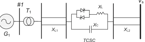
2.1. A Single Machine Infinite Bus System with a TCSC Device

A SMIB system with a TCSC device is shown in Fig. A.1, of which the

system dynamics is described as [24]

⎧ ⎪ ⎪ ⎪ ⎪ ⎪ ⎪ ⎪ ⎪ ⎪ ⎪ ⎨ ⎪ ⎪ ⎪ ⎪ ⎪ ⎪ ⎪ ⎪ ⎪ ⎪ ⎩

˙

δ=_ω−_ω0

˙

ω=−D_H(_ω−_ω0) + ω0

H

Pm− E

qVssinδ

X dΣ+Xtcsc

˙

Eq =

(Xd−Xd)(Vscosδ−Eq)

Td0(XdΣ +Xtcsc) −

1

Td0E

q+TKd0cufd

˙

Xtcsc =−_T1_c(Xtcsc−Xtcsc0) + K_TT_cuc+ζtcsc

(1)

where _δ and _ω denote the angle and relative speed of the generator rotor,

respectively; _H the inertia constant; _Pm the constant mechanical power on

the generator shaft; _Dthe damping coefficient;_Eq and_Vsthe inner generator

voltage and infinite bus voltage; _Td0 the _d-axis transient short-circuit time

constant; _Tc the time constant of TCSC; _XdΣ = _Xt +_Xd + 1

2(XL1+XL2);

Xt the transformer reactance; Xd the d-axis generator transient reactance;

XL1 and XL2 the transmission line reactance;Xtcsc the TCSC reactance and

Xtcsc0 the initial TCSC reactance;Kc the gain of excitation amplifier;ufd the

2.2. A Multimachine System with a TCSC Device

A multimachine system with _n machines and a TCSC device, where the

nth machine is the reference machine, is described by [5]

⎧ ⎪ ⎪ ⎪ ⎪ ⎪ ⎪ ⎪ ⎪ ⎪ ⎪ ⎨ ⎪ ⎪ ⎪ ⎪ ⎪ ⎪ ⎪ ⎪ ⎪ ⎪ ⎩

˙

δi =ωi−ω0

˙

ωi = ₂ω_H0_i

Pmi− D_ω0i(ωi−ω0)−Pei

˙

E_qi = _T1

d0i(ufdi−Eqi), i= 1,2,· · · , n,

˙

Xtcsc =−_T1_c(Xtcsc−Xtcsc0) + K_TT_cuc+ζtcsc

(2)

with

Eqi =Eqi+ (xdi−xdi)Idi

Pei =EqiIqi+Eq2iGii

Idi =−

n

j=1,j=i

E_qjYijcos(δi−δj)

Iqi =−

n

j=1,j=i

EqjYijsin(δi−δj)

where subscript_idenotes the variables of the_ith machine;_δithe relative rotor

angle; _ωi the generator rotor speed; _Eqi and _Eqi the voltage and transient

voltage on the _q-axis; _Pmi the constant mechanical power input; _Pei the

short-circuit time constant; _Idi and _Iqi the _d-axis and _q-axis generator current; _Yij

the equivalent admittance between the _ith and_jth nodes, which is modified

as_Yij = 1_/(1_/Yij+_Xtcsc) when a TCSC is equipped between the_ith and_jth

nodes; and _Gii the equivalent self conductance of the _ith machine.

3. Perturbation Estimation based Coordinated Adaptive Passive

Control

Consider a two input system in formal form of passive system as follows

[19, 21]:

˙

z =_Az+_B(_a(_{z, y}) +_b(_{z, y})_u2+_ξ) (3)

˙

y=_α(_{z, y}) +_β1(_{z, y})_u1+_β2(_{z, y})_u2+_ζ (4)

where _y∈Ris the output and the relative degree from _u1 to_y is one, which

is the basic form in CPC design. _z ∈Rn−1 _{is the state vector of the internal}

dynamics; _a(_{z, y}) : Rn−1 ×R → R _{and b(z, y) :} Rn−1 × R → R _{are C}∞

unknown smooth functions, _ξ ∈ R and _ζ ∈ R are modelling uncertainties.

Matrices _A and _B are A= ⎡ ⎢ ⎢ ⎢ ⎢ ⎢ ⎢ ⎢ ⎢ ⎢ ⎢ ⎢ ⎢ ⎢ ⎢ ⎣

0 1 0 · · · 0

0 0 1 · · · 0

..

. ...

0 0 0 · · · 1

0 0 0 · · · 0

⎤ ⎥ ⎥ ⎥ ⎥ ⎥ ⎥ ⎥ ⎥ ⎥ ⎥ ⎥ ⎥ ⎥ ⎥ ⎦

(n−1)×(n−1)

, B =

⎡ ⎢ ⎢ ⎢ ⎢ ⎢ ⎢ ⎢ ⎢ ⎢ ⎢ ⎢ ⎢ ⎢ ⎢ ⎣ 0 0 .. . 0 1 ⎤ ⎥ ⎥ ⎥ ⎥ ⎥ ⎥ ⎥ ⎥ ⎥ ⎥ ⎥ ⎥ ⎥ ⎥ ⎦

(n−1)×1

The zero dynamics of system (3) is assumed to be stabilizable by _u2 and

written as

˙

z =_Az+_B(_a(_z,0) +_b(_z,0)_u2+_ξ) (5)

3.1. Design of HGSPO and HGPO [5]

The perturbation of system (5) is defined as

Ψ₁(·) =_a(_z,0) + (_b(_z,0)−_b10)_u2+_ξ (6)

Define a fictitious state to represent the system perturbation, that is, _zn =

nth-order system

˙

ze=A1ze+B1u2+B2Ψ˙1(·) (7)

where _ze = [_{z1, z2,}· · · _{, zn−1, zn}]T_{. B}

1 = [0,0, . . . , b10,0]T ∈ Rn and B2 =

[0_,0_{, . . . ,}1]T∈Rn. Matrix _A1 is

A1 =

⎡ ⎢ ⎢ ⎢ ⎢ ⎢ ⎢ ⎢ ⎢ ⎢ ⎢ ⎢ ⎢ ⎢ ⎢ ⎣

0 1 · · · · 0

0 0 1 · · · 0

..

. ...

0 0 0 · · · 1

0 0 0 · · · 0

⎤ ⎥ ⎥ ⎥ ⎥ ⎥ ⎥ ⎥ ⎥ ⎥ ⎥ ⎥ ⎥ ⎥ ⎥ ⎦

n×n

Throughout this paper, ˜_x=_x−_xˆrefers to the estimation error of_xwhereas

ˆ

xrepresents the estimate of _x. A_nth-order HGSPO is used for the extended

nth-order system (7) as

˙ˆ

ze=A1zˆe+B1u2+H(z1−zˆ1) (8)

where _H = [_{α1/, α2/}2_{,· · ·, α}

n−1/n−1, αn/n]T is the observer gain with

The estimation errors of HGSPO (8) is calculated as

˙˜

ze=A1z˜e+B2Ψ˙1(·)−H(z1−zˆ1)

The design procedure of HGSPO can be summarized as following steps:

Step 1: Define the perturbation for system (5) as Eq. (6);

Step 2: Define a fictitious state to represent the perturbation as_zn = Ψ₁(·);

Step 3: Extend the original (n-1)th-order system (5) into the extended

nth-order system (7);

Step 4: Design a nth-order HGSPO (8) to estimate state _z and perturbation

Ψ₁(·) for the extended nth-order system (7);

Step 5: Choose _αi =_Cni_λi such that the pole of HGSPO (8) can be placed at

−λ, where _i= 1_,2_,· · · _{, n} and _{λ >}0.

Similarly, the perturbation of system (4) is defined as

Ψ₂(·) = _α(_{z, y}) +_β2(_{z, y})_u2+ (_β1(_{z, y})−_b20)_u1+_ζ (9)

Ψ₂(·). Then extend the original first-order system (4) into the following

second-order system _⎧

⎪ ⎪ ⎨ ⎪ ⎪ ⎩

˙

y=_y2+_b20u1

˙

y2 = ˙Ψ2(·)

(10)

A second-order HGPO is used for system (10) as

⎧ ⎪ ⎪ ⎨ ⎪ ⎪ ⎩

˙ˆ

y= ˆΨ₂+α1

(y−yˆ) +b20u1

˙ˆ

Ψ₂(·) = α2

2(y−yˆ)

(11)

where 0_{< <}1.

Define the scaled estimation errors of HGPO (11) as_η1 = ˜_y/,_η2 = ˜Ψ₂(·),

and _η = [_{η1, η2}]T_{, gives}

_η˙ =_A1η+_B1Ψ˙₂(·) (12)

with

A₁ =

⎡ ⎢ ⎢ ⎣

−α₁ 1

−α2 0

⎤ ⎥ ⎥

⎦, B₁ =

⎡ ⎢ ⎢ ⎣

0

1

⎤ ⎥ ⎥ ⎦

where _α1 and _α2 are chosen such that _A1 is a Hurwitz matrix.

the pole of HGSPO (8) and HGPO (11) is chosen to be 10 times larger than

the dominant pole of the equivalent linear system of (5) and (4), respectively,

which can ensure a fast estimation of perturbation Ψ₁(·) and Ψ₂(·). Note that

one only needs the measurement of state _z1 and input _u2 for the design of

HGSPO (8), and the measurement of output _yand input_u1 for the design of

HGPO (11). The effectiveness of the PO has been discussed in our previous

work [5, 29, 30].

Remark 1. It should be mentioned that during the design procedure, and

used in HGSPO (8) and HGPO (11) are required to be some relatively

small positive constants only, and the performance of HGSPO and HGPO is

not very sensitive to the observer gains, which are determined based on the

upper bound of the derivative of perturbation.

3.2. Design of stabilizing controller _u2 and coordinated controller _u1

Based on the standard CPC design procedure [19], the stabilizing

con-troller _u2 is designed first as follows:

u2 =γ(ˆze) =

1 b10

which renders system (3) into

˙

z=_Az+_B(_a(_{z, y}) +_b(_{z, y})_γ(ˆ_ze) +_ξ) = ˜_q(_z) + ˜_p(_{z, y})_y

with

˜

q(_z) =_Az+_B(_a(_z,0) +_b(_z,0)_γ(ˆ_ze) +_ξ) (14)

and

˜

p(_{z, y}) =_B(_a(_{z, y})−_a(_z,0) + (_b(_{z, y})−_b(_z,0))_γ(ˆ_ze))_y−1 (15)

where ˜_q(_z) represents the zero dynamics, ˜_p(_{z, y}) denotes the difference

be-tween the original system and zero dynamics, which will be cancelled later

by _u1. _K = [_{k1, k2,}· · · _{, kn−1}] is the control gain which makes matrix_A−_BK Hurwitzian, such that the following condition can be satisfied

˙

W = ∂W(z)

∂zT q˜(z) +

∂W

∂ηTη˙ ≤ −α(z) (16)

The proof of inequality (16) is given in [5].

The structure of stabilizing controller (13) is illustrated in Fig. A.2.

The nominal plant is disturbed by the perturbation Ψ₁(·), the stabilizing

controller _u2 can be separated as _u2 = _b−₁₀1(_us1 +_us2), where _us1 = −_Kzˆis

the state feedback and choose _ki =_Cni_−1ξi to place the pole of the equivalent

linear system of (5) at −_ξ, where _i = 1_{, ..., n}−1 and _{ξ >} 0; and _us2 = −_zˆ_n

compensates the combinatorial effect of parameter uncertainties, external

disturbances and unmodelled dynamics.

The coordinated controller_u1 is designed as

⎧ ⎪ ⎪ ⎨ ⎪ ⎪ ⎩

u1 =b−201

−_Ψˆ

2(·)−ky− _∂z∂WTp˜(z, y) +ν

ν =−_φ(_y)

(17)

where _ν is the additional input,_φ is any smooth function such that_φ(0) = 0

and _yφ(_y)_>0 for all_y= 0. _{k >}1 is the feedback control gain.

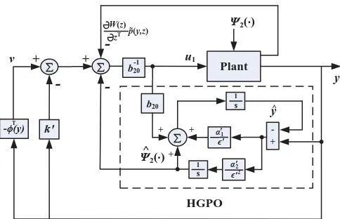
The structure of coordinated controller (17) is illustrated in Fig. A.3.

The nominal plant is disturbed by the perturbation Ψ₂(·), the coordinated

controller _u1 can be separated as _u1 = _b−₂₀1(_uc1 +_uc2 +_uc3 +_uc4), where

uc1 = −Ψˆ2(·) is the dynamical perturbation compensation; uc2 = −ky

uc3 = _∂z∂WTp˜(y, z) coordinates the two controllers by cancelling the difference

between the original system and zero dynamics represented by ˜_p(_{y, z}); and

uc4 = ν constructs a passive system by introducing an additional input in

the form of a sector-nonlinearity _φ(_y).

Remark 2. Note that ∂W_∂z(Tz)p˜(z, y) = ∂W_∂zn(₋z₁)p˜n−1(z, y) as ˜pi(z, y) = 0, i =

1_,2_,· · ·_{, n} −2, which can be interpreted as the distributed energies in a

complex system and needs to be reshaped. One can choose ∂W_∂z(Tz)p˜(z, y) =

czn−1p˜n−1(z, y) regardless of the system order, where c is called the

coordi-nation coefficient.

Remark 3. For the closed-loop system (18), control gain _k should be

de-signed to suppress the perturbation estimation error ˜Ψ₂(·). Compared to the

approach without perturbation compensation, in which _k should be chosen

to suppress the perturbation Ψ₂(·). As Ψ₂(·) is normally larger than ˜Ψ₂(·),

a smaller_k could be resulted in due to the compensation of perturbation by

PECAPC.

To this end, PECAPC design for systems (3) and (4) can be summarized

as:

Step 2: Extend system (5) into system (7), and design HGSPO (8) to obtain

estimates ˆ_z and ˆ_zn

Step 3: Design stabilizing controller (13)

Step 4: Extend system (4) into system (10), and design HGPO (11) to obtain

the estimate ˆΨ₂(·)

Step 5: Design coordinated controller (17)

3.3. Closed-loop system stability

The proof of stability of the closed-loop system with control stabilizing

controller_u2 and coordinated controller_u1 is given in the following Theorem

1.

Theorem 1. Consider systems (3) and (4), with controllers (13) and (17),

and let assumptions A1 and A2 hold; then ∃∗₁, ∗_{1 >} 0 such that, ∀, 0 _<

< ∗1, then the closed-loop system is passive and its origin is stable.

The following assumptions are made on systems (7) and (10).

A1. _b10 and _b20 are chosen to satisfy:

where _{θ1 <}1 and _{θ2 <}1 are positive constants.

A2. The perturbation Ψ_k(·) and its derivative ˙Ψ_k(·) are Lipschitz in their

arguments and bounded over the domain of interest and are globally bounded

in (_{z, y}):

|Ψ_k(_{z, y, u})| ≤_γ1, |Ψ˙_k(_{z, y, u})| ≤_γ2

where_γ1and_γ2are positive constants. In addition, Ψ_k(0_,0_,0) = 0, ˙Ψ_k(0_,0_,0) =

0,_k = 1_,2. It guarantees that the origin is an equilibrium point of the

open-loop system.

Proof. The closed-loop system (4) using controller (17) is

⎧ ⎪ ⎪ ⎨ ⎪ ⎪ ⎩

˙

y =_η2 −_ky− ∂W_∂zT(z)p˜(z, y) +ν

η˙ =_A1η+_B1Ψ˙₂(·)

(18)

Define a Lyapunov function_V(_η) =_ηT_P

1η, where P1 is the positive definite

solution of the Lyapunov equation _P1A1 +_AT

1 P1 = −I. For closed-loop

as

H(_{z, η, y, η}) =_W(_{z, η}) + 1

2y

2_{+βV(η) (19)}

where _{β >}0. Moreover, assuming

_Ψ˙

2(·) ≤L1y+L2η

where _L1 and _L2 are Lipschitz constants.

By differentiating _H(_{z, η, y, η}) along the trajectory of system (18) and

condition (16), it yields

˙

H = ∂W

∂zT(˜q(z) + ˜p(z, y)y) +

∂W

∂ηTη˙+y

η2 −ky−

∂W

∂zTp˜(z, y) +ν

+_β ∂V

∂ηT

A1η

+B

1Ψ˙2(·)

≤ −α(_z) +_yν− _y2− β

η

2_{+ 2βL2P1η}2_{+ (1 + 2βL1P1)yη}

≤ −α(_z) +_yν− _y2− β

η

2_{+ 2βL2P1η}2_{+ (1 + 2βL1P1)}

×

1 0

y2+_0η2

≤ −α(_z) +_yν− 1

2y

2₋ β

2η

2_−b

where

b1 =

1

2 −

2 0

1

2 +βL1P1

, b2 = β

2 −2β(0L1 +L2)P1 −0

with _{0 >} 0. One can choose _β small enough and ₀ ≥ ∗₀ = 2 + 4_βL1_P1

such that _{b1 >} 0, then choose ∗₁ = _β/(∗2

0 + 4βL2P1), ∀, ≤ ∗1, and

choose the additional input _ν = −_φ(_y), where _φ(_y) is a sector-nonlinearity

satisfying _yφ(_y)_>0. It can be shown that

˙

H ≤ −α(_z)−min(1_/2_{, β/}2)(_y2+_η2) +_yν ≤ −_α(_z)−_α1(_y) +_yν

≤yν ≤ −yφ(_y)≤0

where_α1 is a class-Kfunction. One can conclude that the closed-loop system

is passive and its origin is stable.

Proposition 1. PECAPC can be easily extended into multi-input systems.

If there exists_msubsystems for system (3) with_mcontrol inputs_u2j, the

vec-tor variables of states and estimation errors for each subsystem are denoted

per-turbation. Hence _u2j can stabilize the _jth subsystem, which results in an

equivalent CLF _W(_z∗_{, η}∗) = _W1 +_W2 +· · ·+_Wm, and condition (16)

be-comes

˙

W =

m

j=1

∂W ∂z∗T

j ˜

qj(zj∗) + _∂η∂W∗T

j ˙ η_j∗

≤m

j=1

αj(zj∗)

Remark 4. Denote (_{z0, y0}) ∈ Γ_o and _z0 ∈ Γ_z as the equilibrium point of

systems (3) and (5), respectively, where Γ_o and Γ_z are their stability

re-gion, which are unequal during transient process. However, with a proper

coordination coefficient _c, passive controller (17) will exponentially drive

lim_t→∞(_{z0, y0}) =_z0 and lim_t→∞Γ_o = Γ_z as lim_t→∞y = 0.

Remark 5. Compared to the CAPC [24, 25] which usually estimates the

linearly parametric uncertainties, the PECAPC can be regarded as a

non-linearly functional estimation method, as it can estimate the combinatorial

effect of fast time-varying unknown parameters, unknown nonlinear dynamics

and external disturbances. If there does not exist uncertainties and external

disturbances, and if the accurate system model is available, such a controller

provides the same performance as the exact passive controller. Otherwise,

The use of PO leads to less concern over the measurement and identification

of the fast time-varying unknown parameters, unknown nonlinear dynamics

and external disturbances. This tends to require less control efforts as the

perturbation has already included all of this information.

4. PECAPC Design of Excitation and TCSC

Controllers (13) and (17) will be applied for both SMIB system (1) and

multimachine system (2).

4.1. Controller Design for a Single Machine Infinite Bus System

For SMIB system (1), we chose _y=_Xtcsc−_Xtcsc0, _u1 =_uc and _u2 =_ufd.

By setting _y = 0, the zero dynamics of system (1) is

⎧ ⎪ ⎪ ⎪ ⎪ ⎪ ⎪ ⎨ ⎪ ⎪ ⎪ ⎪ ⎪ ⎪ ⎩

˙

δ =_ω−_ω0

˙

ω =−D_H(_ω−_ω0) + ω0

H

Pm− E

qVssinδ

X

dΣ+Xtcsc0

˙

E_q = (Xd−Xd)(Vscosδ−Eq)

Td0(XdΣ +Xtcsc0) −

1

Td0E

q+TKd0cufd

(20)

Choose _z1 = _δ −_δ0 for system (20), where _δ0 is the initial generator

explicitly, the system perturbation Ψ₁(·) is obtained as

Ψ₁(·) =−D H

−D

H(ω−ω0) +

ω0

H

Pm−

EqVssinδ

X_dΣ +_Xtcsc0

− ω0Vs

H(_XdΣ +_Xtcsc0)

×Eq(ω−ω0) cosδ+

sin_δ

Td0

(_Xd−_Xd)(_Vscos_δ−_Eq) (_XdΣ +_Xtcsc0) −E

q

− ω0Vssinδ

H(_XdΣ +_Xtcsc0) ×

Kc

Td0ufd

−b10ufd (21)

Defining a fictitious state as _z4 = Ψ₁(·), and the extended state variable is

denoted as _ze = [_{z1, z2, z3, z4}]T_{, the fourth-order state equation is}

˙

ze=A1ze+B1ufd+B2Ψ˙1(·) (22)

where

A1 =

⎡ ⎢ ⎢ ⎢ ⎢ ⎢ ⎢ ⎢ ⎢ ⎢ ⎢ ⎣

0 1 0 0

0 0 1 0

0 0 0 1

0 0 0 0

⎤ ⎥ ⎥ ⎥ ⎥ ⎥ ⎥ ⎥ ⎥ ⎥ ⎥ ⎦

, B1 =

⎡ ⎢ ⎢ ⎢ ⎢ ⎢ ⎢ ⎢ ⎢ ⎢ ⎢ ⎣ 0 0 b10 0 ⎤ ⎥ ⎥ ⎥ ⎥ ⎥ ⎥ ⎥ ⎥ ⎥ ⎥ ⎦

, B2 =

A fourth-order HGSPO (8) is given as ⎧ ⎪ ⎪ ⎪ ⎪ ⎪ ⎪ ⎪ ⎪ ⎪ ⎪ ⎨ ⎪ ⎪ ⎪ ⎪ ⎪ ⎪ ⎪ ⎪ ⎪ ⎪ ⎩ ˙ˆ

z1 = ˆz2+α1(z1−zˆ1)

˙ˆ

z2 = ˆz3+α22(z1−zˆ1)

˙ˆ

z3 = ˆΨ1(·) + α33(z1 −zˆ1) +b10ufd

˙ˆ

Ψ₁(·) = α4

4(z1−zˆ1)

(23)

Extending the TCSC dynamics, it yields

⎧ ⎪ ⎪ ⎨ ⎪ ⎪ ⎩ ˙

y= Ψ_tcsc(·) +_b20uc

˙

y2 = ˙Ψtcsc(·)

(24)

where

Ψ_tcsc(·) =− 1

Tcy

+KT

Tc uc

−b20uc+ζtcsc (25)

A second-order HGPO (11) is used to obtain ˆΨ_tcsc(·) as

⎧ ⎪ ⎪ ⎨ ⎪ ⎪ ⎩ ˙ˆ

y= ˆΨ_tcsc(·) + α1

(y−yˆ) +b20uc

˙ˆ

Ψ_tcsc(·) = α2

2(y−yˆ)

For system (1), one can obtain ˜_p(_{z, y}) from (21) according to (15) as

˜

p(_{z, y}) = ω0Vs

H

₁

XΔ

_−DE

qsinδ

H +E

q(ω−ω0) cosδ+

sin_δ

Td0 ×

(−_Eq +_Kcufd)

+X

Δ

X2

Δ

(_Xd−_Xd)(_Vscos_δ−_Eq) sin_δ Td0

(27)

where_XΔ= (_XdΣ +_Xtcsc0+_y)(_XdΣ +_Xtcsc0) and_XΔ = (2_XdΣ + 2_Xtcsc0+_y).

The PECAPC-based EC and TCSC controller are

⎧ ⎪ ⎪ ⎪ ⎪ ⎪ ⎪ ⎨ ⎪ ⎪ ⎪ ⎪ ⎪ ⎪ ⎩

ufd= _b1₁₀(−Ψˆ1(·)−k1zˆ3−k2zˆ2 −k3zˆ1)

uc= _b1₂₀(−Ψˆtcsc(·)−czˆ3p˜(z, y)−ky+ν)

ν=−_βy

(28)

A known ˜_p(_{z, y}) is a fundamental assumption in coordinated passive control

design [19], which contains the system states and parameters and needs to be

cancelled for passivation. In real power system operations, the damping

coef-ficient _D is small compared to the system inertia _H thus|_DEq sin_δ/H| ≈0,

and |XΔ

X2 Δ

(_Xd−_Xd)(_Vscos_δ−_Eq)| | −_Eq +_Kcufd|during the transient

pro-cess due to the large excitation control input _ufd, thus one can approximate

˜

approximation, it gives

˜

p∗(_{z, y}) = ω0Vs

HXΔ

E_q(_ω−_ω0) cos_δ+ sinδ Td0

(−_Eq +_Kcufd)

(29)

To this end, we replace ˜_p(_{z, y}) by its approximation ˜_p∗(_{z, y}), controller (28)

becomes ⎧

⎪ ⎪ ⎪ ⎪ ⎪ ⎪ ⎨ ⎪ ⎪ ⎪ ⎪ ⎪ ⎪ ⎩

ufd= _b1₁₀(−Ψˆ1(·)−k1zˆ3−k2zˆ2 −k3zˆ1)

u∗_c = _b1

20(−

ˆ

Ψ_tcsc(·)−_czˆ_3p˜∗(_{z, y})−_ky+_ν)

ν=−_βy

(30)

Based on assumption A1, constants _b10 and _b20 must satisfy following

in-equalities when the generator operates within its normal region:

b10<−ω0VsKcsinδ/[2HTd0(XdΣ +Xtcsc0)]

b20> KT/(2Tc)

During the most severe disturbance, the electric power will reduce from its

initial value to around zero within a short period of time, Δ. Thus the

boundary values of the estimated system states can be obtained as |_zˆ3| ≤

4.2. Controller Design for a Multimachine System

For multimachine system (2), we choose _y =_Xtcsc −_Xtcsc0, _u1 =_uc and

u2i = ufdi. Setting y = 0 in the equivalent admittance matrix Y, the zero

dynamics can be obtained. Choose _zi1 = _δi −_δi0, _i = 1_,2_{, . . . , n}, where

δi0 is the initial rotor angle of the ith generator. Differentiatingzi1 until the

excitation control input_ufdiappears explicitly, the system perturbation Ψ_i(·)

is obtained as

Ψ_i(·) =− ω0 2_Hi

_D

i ω0

dωi

dt +E

qi

dIqi

dt +

Iqi+ 2GiiEqi

Td0i

(−_Eqi−(_xdi−_xdi)_Idi)

− ω0(Iqi+ 2GiiEqi)

2_HiTd0i ufdi−b10iufdi (31)

Defining a fictitious state as _zi4 = Ψ_i(·), and the extended state variable is

denoted as _zie= [_{zi1, zi2, zi3, zi4}]T, the fourth-order state equation is

˙

where

Ai1 =

⎡ ⎢ ⎢ ⎢ ⎢ ⎢ ⎢ ⎢ ⎢ ⎢ ⎢ ⎣

0 1 0 0

0 0 1 0

0 0 0 1

0 0 0 0

⎤ ⎥ ⎥ ⎥ ⎥ ⎥ ⎥ ⎥ ⎥ ⎥ ⎥ ⎦

, Bi1 =

⎡ ⎢ ⎢ ⎢ ⎢ ⎢ ⎢ ⎢ ⎢ ⎢ ⎢ ⎣ 0 0

b10i

0 ⎤ ⎥ ⎥ ⎥ ⎥ ⎥ ⎥ ⎥ ⎥ ⎥ ⎥ ⎦

, Bi2 =

⎡ ⎢ ⎢ ⎢ ⎢ ⎢ ⎢ ⎢ ⎢ ⎢ ⎢ ⎣ 0 0 0 1 ⎤ ⎥ ⎥ ⎥ ⎥ ⎥ ⎥ ⎥ ⎥ ⎥ ⎥ ⎦

A fourth-order HGSPO (8) is used for the ith generator as

⎧ ⎪ ⎪ ⎪ ⎪ ⎪ ⎪ ⎪ ⎪ ⎪ ⎪ ⎨ ⎪ ⎪ ⎪ ⎪ ⎪ ⎪ ⎪ ⎪ ⎪ ⎪ ⎩ ˙ˆ

zi1 = ˆzi2+αi1(zi1−zˆi1)

˙ˆ

zi2 = ˆzi3+αi22(zi1−zˆi1)

˙ˆ

zi3 = ˆΨi(·) + αi33(zi1−zˆi1) +b10iufdi

˙ˆ

Ψ_i(·) = αi4

4 (zi1−zˆi1)

(33)

Let us consider the equivalent two-machine subsystem involving the TCSC

device and denote them as the_jth and_kth machine, namely, the TCSC device

is installed between the _jth and _kth machine. Furthermore, each machine

denoted by the _ith machine is equipped with its own EC. The extended

TCSC dynamics is the same as system (24), and the same HGPO (26) is

The PECAPC-based EC and TCSC controller for system (2) is

⎧ ⎪ ⎪ ⎪ ⎪ ⎪ ⎪ ⎨ ⎪ ⎪ ⎪ ⎪ ⎪ ⎪ ⎩

ufdi= _b101_i(−Ψˆi(·)−ki1zˆi3−ki2ˆzi2−ki3zˆi1)

uc= _b1₂₀(−Ψˆtcsc(·)−cjzˆj3p˜j(z, y)−ckzˆk3p˜k(z, y) +ν)

ν =−_{βy, i}= 1_,2_,· · · _{, n}

(34)

where ˜_pj(_{z, y}) and ˜_pk(_{z, y}) are calculated from (31) according to (15), in which

TCSC device is installed between the_jth and_kth machine. Thus one chooses

i =_j and _i =_k in (31) to calculate ˜_pj(_{z, y}) and ˜_pk(_{z, y}), respectively, using

the values given in Appendix A. Similarly, in real power system operations,

|DjEqjEqksinδjk/(2Hj)| ≈ 0 as damping coefficient Dj Hj, |

2Gjj

Td0j(xdj −

xdj)| |ωjk|as the self conductance Gjj is much smaller than time constant

Td0j. Moreover|(xdk−xdk)(

_n

i=1,i=k,jEqiYkicosδki+

X∗ Δ

X∗

ΔE

qjcosδjk)| |ufdk−

E_qk|and |(_xdj −_xdj)(_in_{=1,i=j,kEqiYji}cos_δji+ XΔ∗

X∗

ΔE

qkcosδkj)| |ufdj−Eqj|

during the transient process due to the large excitation control inputs _ufdk

and _ufdj, thus one can approximate ˜_pj(_{z, y}) and ˜_pk(_{z, y}) by ignoring the

˜

p∗_j(_{z, y}), respectively, gives

˜

p∗_j(_{z, y}) = ω0X

∗

Δ

2_Hj

_E

qk

Td0j

(_ufdj−_Eqj) sin_δjk+ E

qj

Td0k

(_ufdk−_Eqk) sin_δjk

+_EqjEqkωjkcos_δjk

˜

p∗_k(_{z, y}) = ω0X

∗

Δ

2_Hk

_E

qj

Td0k

(_ufdk−_Eqk) sin_δkj+ E

qk

Td0j

(_ufdj−_Eqj) sin_δkj

+_EqkEqjωkjcos_δkj

As a result, one can replace ˜_pj(_{z, y}) and ˜_pk(_{z, y}) by their approximation

˜

p∗_j(_{z, y}) and ˜_p∗_k(_{z, y}), respectively. Controller (34) becomes

⎧ ⎪ ⎪ ⎪ ⎪ ⎪ ⎪ ⎨ ⎪ ⎪ ⎪ ⎪ ⎪ ⎪ ⎩

ufdi = _b101_i(−Ψˆi(·)−ki1zˆi3−ki2zˆi2−ki3zˆi1)

u∗_c = _b1

20(−

ˆ

Ψ_tcsc(·)−_cjzˆ_j3p˜∗_j(_{z, y})−_ckzˆ_k3p˜∗_k(_{z, y}) +_ν) ν =−_{βy, i}= 1_,2_,· · · _{, n}

(35)

Similar to the SMIB case, constants _b10i and _b20 are chosen to be:

b10i <−ω0(Iqi+ 2GiiEqi)/(2HiTd0i)

Moreover, estimates of state and perturbation are bounded as|_zˆ_i3| ≤_ω0Pmi/(2_Hi),

|_Ψˆ_{i(·)| ≤ω}

0Pmi/(2HiΔ), and |Ψˆ˙i(·)| ≤ω0Pmi/(2HiΔ2).

To this end, a decentralized EC can be obtained for the _ith machine as

only the measurement of its rotor angle _δi is required, which can effectively

handle the modelling uncertainties. The TCSC controller measures the rotor

angles _δj and _δk, excitation control inputs _ufdj and _ufdk, transient voltages

E_qj and _Eqj. The nominal values of time constant _Td0j and _Td0k, inertial

constants _Hj and _Hk of the _jth and _kth machine, and transmission line

reactance_Xjkare used for coordination. Note that the difference between the

nominal values and the real values of the system parameters are aggregated

into the perturbation, which is estimated by PO.

5. Simulation Results

5.1. Evaluation on a Single Machine Infinite Bus System

A proportional-integral-derivative (PID) based TCSC controller and

au-tomatic voltage regulator equipped with lead-lag (LL) based PSS (PID+LL),

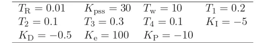
CAPC used in [24], and PECAPC are compared. The system parameters and

initial operating conditions are given in Appendix A. Through trial-and-error,

and dynamical performance. PECAPC parameters are chosen as: _k1 = 9,

k2 = 27, k3 = 27 so as to place the poles of the linear system at ξ = −3;

b10 = −15, b20 = 100, k = 5, β = 15, c= 0.001; α1 = 160, α2 = 9.6×103,

α3 = 2.56× 105 and α4 = 2.56×106 so as to place all the poles of the

HGSPO at _λ = −40; _α1 = 30 and _α2 = 225 so as to place all the poles of

the HGPO at _λ = −15, = 0_.1 and Δ = 0_.05 _s. The system variables are

used in the per unit (p.u.) system. In the power systems analysis field of

electrical engineering, per unit system is the expression of system quantities

as fractions of a defined base unit quantity, which means the values have

been normalized [1]. In this paper, assume the independent base values are

active power _Pbase=1.0 p.u. and voltage _Vbase=1.0 p.u..

A three-phase short circuit fault occurs at_t= 1_.0_sand cleared at_t= 1_.1

s, where|_ufd| ≤7 p.u., and|_Xtcsc| ≤0_.1 p.u. such that a maximum 20%

com-pensation ratio is implemented. Figure A.4 shows system responses with the

EC alone, coordinated EC and TCSC controller (28) and its approximated

controller (30), respectively. From which the effectiveness of coordination is

verified as an extra system damping is injected, and the excitation control

cost is reduced. Moreover, the approximation is valid as it can capture the

will be used for the rest of the studies.

System responses under the nominal model is illustrated by Fig. A.5. It is

found that PECAPC can effectively stabilize the system. Figure A.6 presents

system responses under a nonlinear unmodled TCSC dynamics _ζtcsc =

10 sin(_Xtcsc −_Xtcsc0), which is the same unmodelled TCSC dynamics used

in [24] for the purpose of their control performance evaluation. However,

PECAPC does not require the model error to satisfy this linear growth

con-dition required by CAPC [24]. In fact, a general unmodelled TCSC dynamics

can be estimated online by PO. PID+LL control performance degrades

dra-matically as it is not robust to the TCSC modelling uncertainty. In contrast,

both CAPC and PECAPC can maintain a consistent control performance as

this uncertainty is considered during control design.

The low frequency inter-area oscillation has been well defined in the power

system research, which is caused by the dynamic interactions, in a low

fre-quency, between multiple groups of generators. It results in a degrade of

power system stability and must be suppressed. A typical inter-area

oscilla-tion_Vs= 1 + 0_.1 sin(5_t) is chosen to an corresponding oscillation frequency of

(2_.5_/π) Hz. System responses are given in Fig. A.7, the control performance

contrast, PECAPC can effectively attenuate the inter-area oscillation.

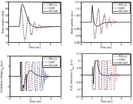
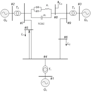
5.2. Evaluation on a Three-Machine System

The PID+LL, CPC, where the real value of the states and

perturba-tion is used in the controllers, and PECAPC (35) are then evaluated on a

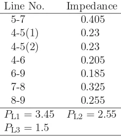
three-machine nine-bus system as shown in Fig. A.8, where a TCSC device

is equipped between bus #7 and bus #8. The system parameters, initial

operating conditions and PID+LL parameters are all given in Appendix A.

PECAPC parameters are _b10i =−30, _ki1 = 15, _ki2 = 75, _ki3 = 125 so as to

place the poles of the linear system at _ξ =−5; _b20 = 20, _k = 10, _β = 1 and

c2 =c3 = 0.25; αi1 = 200,αi2 = 1.5×104,αi3 = 5×105 and αi4 = 6.25×106

so as to place all the poles of the HGSPO at_λ=−40; _α1 = 60 and_α2 = 900

so as to place all the poles of the HGPO at _λ =−30, = 0_.1 and Δ = 0_.05

s.

A three-phase short circuit occurs on one transmission line between bus

#4 and bus #5 marked as point × at_t = 0_.5_s, the faulty transmission line

is switched off at _t= 0_.6_s, and switched on again at_t = 1_.1_swhen the fault

is cleared, where |_ufdi| ≤7 p.u., and |_Xtcsc| ≤0_.2 p.u. such that a maximum

System responses under operation type I are given by Fig. A.9, which

shows PECAPC can achieve as satisfactory control performance as that of

CPC when an accurate system model is completely known, their tiny

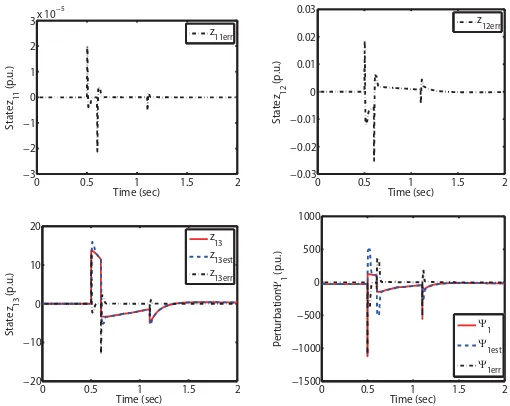
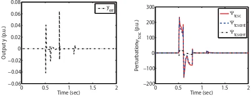
dif-ference is caused by the estimation error. The observer performance during

the fault is also monitored, the estimation errors of HGSPO₁ and HGPO are

given in Fig. A.10 and Fig. A.11, respectively, which show the observers

can provide accurate estimates of system states with a fast tracking rate.

However, there exists relatively larger errors in the estimate of perturbation

at the instant of _t = 0_.5 _s, _t = 0_.6 _s, and _t = 1_.1 _s, this is due to the

discontinuity in the equivalent admittance _Y12 caused by the disconnection

and reconnection of the transmission line 4-5(2) at the instant when the fault

occurs.

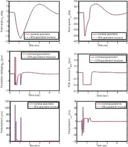
A 50% increase of the generator inertia_Hi, time constant_Td0i and TCSC

time constant_Tc used in controller (35) has been tested to evaluate the effect

of parameter uncertainties on the dynamic response of the proposed control

scheme with and without the PO. Fig. A.12 shows that the control

per-formance degrades dramatically in the presence of parameter uncertainties

without the PO, in contrast the same control performance can be achieved

uncer-tainties of the generator inertia _Hi and time constant _Td0i are included in

perturbation Ψ_i(·) (31), which is estimated by HGSPO (33) and compensated

by controller (35). While the parameter uncertainties of the TCSC time

con-stant _Tc are included in perturbation Ψ_tcsc(·) (25), which is estimated by

HGPO (26) and compensated by controller (35).

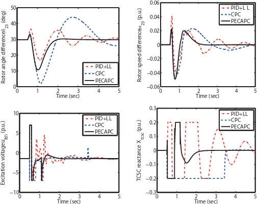
The robustness of PID+LL, CPC and PECAPC has been evaluated by

reducing the inertia constant _Hi, time constant _Td0i of all generators and

TCSC time constant_Tc by 30% from their nominal values. System responses

are provided in Fig. A.14, in which a big difference in CPC has been

iden-tified, with and without accurate parameters. By contrast, PID+LL and

PECAPC remain satisfactory control performance as their design does not

require accurate system parameters.

In order to test the general effectiveness of PECAPC, Figure A.15 presents

system responses obtained with operation Type II and the above parameter

uncertainties. In this case a larger active power is transmitted, and the

system suffers more severe oscillation when the fault occurs. One can find

PID+LL control performance degrades dramatically as its control

parame-ters are based on local system linearization. On the other hand, a severe

contrast, PECAPC can maintain consistent control performance and provide

significant robustness.

6. Hardware-in-the-loop Test

A HIL test has been undertaken based on dSPACE systems to verify the

implementation feasibility of PECAPC. The configuration and experiment

platform of HIL test are shown in Fig. A.17 and Fig. A.18, respectively.

The EC and the TCSC controller are implemented on one dSPACE platform

(DS1104 board) with a sampling frequency_fc= 1 kHz, and the SMIB system

is simulated on another dSPACE platform (DS1006 board) with a sampling

frequency_fs = 10 kHz. The measurements of the rotor angle_δ, rotor speed_ω,

inner generator voltage_Eq, infinite bus voltage_Vs and TCSC reactance _Xtcsc

are obtained from the real-time simulation of SMIB system on the DS1006

board, which are sent to two controllers implemented on the DS1104 board

for calculating the control outputs, i.e., excitation voltage _ufd and TCSC

modulated input _uc, respectively.

The disturbance is set up as: A 0.1 _s three-phase short circuit fault

occurs at 1.9 _s. The total experiment time is 60 _s and only the result of the

following three tests are carried out: Test 1: Same observer parameters used

in the previous simulation, which poles _λ = 40, _λ = 15 with _b10=−15 and

b20 = 100; Test 2: Reduced observer poles λ= 15, λ = 15 with b10 =−150

and _b20 = 200; and Test 3: Further reduced observer poles _λ = 5, _λ = 5

with _b10=−150 and_b20 = 200.

It has been found from Test 1 that an unexpected high-frequency

os-cillation occurs in _ufd and _Xtcsc, which does not appear in the simulation.

This is due to the large observer poles result in high gains, which lead to

highly sensitive observer dynamics to the measurement disturbances. Hence

reduced observer poles are chosen in Test 2. Fig. A.19 shows that the rotor

angle and speed can be effectively stabilized, but a consistent high-frequency

oscillation still exists in both _ufd and _Xtcsc. Through the trial-and-error it

finds that an observer pole in the range of 3-10 can avoid the high-frequency

oscillation but with almost similar transient responses, therefore the observer

poles are further reduced in Test 3. The system transient responses obtained

in simulation and HIL test are given by Fig. A.20, one can find that the

high-frequency oscillation disappears and the rotor angle and speed are still

effectively stabilized.

is possibly caused by the following two reasons: (a) There exists measurement

disturbances in the HIL test which are not considered in the simulation, a

filter could be used to remove the measurement disturbances and improve the

control performance; and (b) The discretization of the HIL test and sampling

holding may introduce an additional amount of error compared to continuous

control used in the simulation.

7. Discussion

It is necessary to study the computational cost of PECAPC as the high

performance systems often have high computational cost. As the PECAPC

needs to calculate a fourth-order HGSPO (23) and a second-order HGPO

(26) together with a nonlinear function (29), it has the highest computational

cost. The computational cost of CAPC is higher than that of CPC, as CAPC

requires to solving an additional second-order parameter estimator (A.1).

For CPC and PID+LL, it’s difficult to compare the computational cost as

CPC has to calculate three complex functions (21), (25) and (29), while

PID+LL has to calculate a first-order integral used in PID, and a

second-order lead-lag plus a first-second-order washout loop used in LL. For the

(21), (25) and (29) become more complex) and PECAPC (nonlinear function

(29) becomes more complex) will be higher than that of the SMIB system,

while the computational cost of PID+LL does not change. As the PECAPC

is a decentralized controller, it can be easily extended into multimachine

systems as each generator will be equipped with an individual EC, and the

TCSC controller is separately implemented in the TCSC device.

Finally, the majority of studies related to power system control and

op-eration is so far based on the simulation. The paper is concerned with the

investigation of a new control method, for which it is difficult to undertake a

physical experiment for the multi-machine power system due to its significant

scale and complexity.

8. Conclusion

In this paper, a novel PECAPC has been proposed for synchronous

gen-erators and TCSC devices to improve the power system stability. It is able to

fully exploit the physical properties of power systems through reshaping the

distributed energies, and handle system uncertainties, unmodelled

dynam-ics and external disturbances via perturbation estimation. The simulation