Accessibility of the resources of near Earth space using
multi-impulse transfers
Joan-Pau Sanchez* and Colin R. McInnes†
Advanced Space Concepts Laboratory, University of Strathclyde, Glasgow, UK
Most future concepts for exploration and exploitation of space require a large initial mass in low Earth orbit. Delivering this mass requires overcoming Earth’s natural gravity well, which imposes a distinct obstacle to space-faring. An alternative for future space progress is to search for resources in-situ among the near Earth asteroid population. This paper examines the scenario of future utilization of asteroid resources. The near Earth asteroid resources that could be transferred to a bound Earth orbit are determined by integrating the probability of finding asteroids inside the Keplerian orbital element space of the set of transfers with an specific energy smaller than a given threshold. Transfers are defined by a series of impulsive maneuvers and computed using the patched-conic approximation. The results show that even moderately low energy transfers enable access to a large mass of resources.
Nomenclature
a = semi-major axis of an orbit, AUb = exponent parameter of power law size distribution, 2.354 C = constant parameter of power law size distribution, 942 D = asteroid diameter, km or m
e = eccentricity of an orbit
f = portion of material with {a,e,i} capturable with an insertion v lower than a given limit H = absolute magnitude
h = percentage of {a,e,i}-orbits that can be phased with the Earth with a v lower than a limit i = inclination of an orbit, deg
m = mass of the asteroid, kg M = mean anomaly of an orbit, deg
M[Du-Dlo]= total asteroid mass between upper and lower diameter, kg
MOIDcap= maximum MOID at which a perigee insertion is possible with a given maneuver, AU. N = number of asteroids
p = semi-latus rectum of an orbit, AU
P = probability of finding an capturable asteroid within a volume in Keplerian element space {a,e,i} ra = apoapsis altitude, AU
renc = distance from the Sun of the intersection point, AU
rp = periapsis altitude, AU
e
t = time at the encounter or intersection point, s
m
t = time of the phasing maneuver, s enc
n
v = normal Cartesian component of the orbital velocity at the intersection point, AU/s
enc r
v = radial Cartesian component of the orbital velocity at the intersection point, AU/s
plX
v = asteroid velocity at the Earth plane crossing point, AU/s
0
v = orbital velocity of the asteroid, AU/s
* [email protected], member AIAA, Research Fellow, Advanced Space Concepts Laboratory, Department of Mechanical Engineering, University of Strathclyde, Glasgow
†
v = hyperbolic excess velocity, AU/s
∆i = inclination change of the asteroid, deg
∆M = difference in mean anomaly of the asteroid, deg ∆n = change of asteroid mean motion, rad/s
v
= increment of velocity
inc
v
= impulsive v to change asteroid inclination, AU/s
cap v
= v for final Earth capture, AU/s
∆vlev = delta-velocity-v∞ leveraging maneuver, AU/s
.
thres
v
= maximum allowed v, AU/s a
= semi-major axis change due to an impulse maneuver, AU
t
v
= tangential impulse provided by phasing maneuver, AU/s α = flight path angle, rad or deg
= true anomaly of an orbit, rad or deg
enc
= true anomaly of the intersection point, rad or deg
= gravitational constant of the Earth, 1.19069x10⁻¹⁹AU3/s2Sun
= gravitational constant of the Sun, 3.96438x10⁻¹⁴AU3/s2
.
= probability density functiona
= asteroid density, kg/m3
= argument of the ascending node of an orbit, rad or deg
= argument of the perigee of an orbit, rad or deg
= Earth‟s mean angular velocity, rad/sωMOID0= periapsis argument at which MOID is zero
Suffixes:
| = referent to Earth
max
| = maximum value allowed
min
| = minimum value allowed
Acronyms:
MOID = Minimum Orbital Intersection Distances NEA = Near Earth Asteroid
I.
Introduction
ost of the plausible futures for human space exploration and exploitation involve a large increase of mass in Earth orbit. Examples include space solar power, space tourism or more visionary human space settlements. Whether this mass is water for crew, propellant for propulsion or materials for structures, these resources will require overcoming Earth‟s natural gravity well to be delivered in space. Thus, even if technologically possible, this will certainly put a large economic burden to future space progress. An alternative to this approach is to search among the population of asteroids in search of the required reservoir of material1.
Asteroids are of importance in uncovering the formation, evolution and composition of the solar system. In particular, near Earth asteroids (NEA) have rose in prominence because of two important points: they are among the easiest celestial bodies to reach from the Earth and they may represent a long-term threat2. The growing interest in these objects has translated into an increasing number of missions to NEA, such as the sample return missions Hayabusa3 and Marco Polo4, impactor missions such as Deep Impact* and possible deflector demonstrator missions such as Don Quixote†.
With regard to asteroid deflection, a range of methods have been identified to provide a change in the asteroid linear momentum5. Some of these methods, such as the kinetic impactor have been deemed to have a high technology readiness level (TRL), while others may require considerable development. If the capability to impact an asteroid exists (e.g., Deep Impact), or if the capability to deflect an asteroid is available in the near future, a
*
http://www.nasa.gov/mission_pages/deepimpact/main/index.html † http://www.esa.int/SPECIALS/NEO/SEMZRZNVGJE_0.html
resource-rich asteroid could in principle be maneuvered and captured into a bound Earth orbit through judicious use of orbital dynamics. On the other hand, if direct transfer of the entire NEA is not possible, or necessary, extracted resources could also be transferred to a bound Earth for utilization. It is envisaged that NEA could also be „shepherded‟ into easily accessible orbits to provide future resources.
The main advantage of asteroid resources is that the gravity well from which materials would be extracted is much weaker than that of the Earth or the Moon. Thus, these resources could in principle be placed in a weakly-bound Earth orbit for a lower energy cost than material delivered from the surface of the Earth or Moon. The question that arises then is how much near-Earth asteroid material is there which can be captured with a modest investment of energy. This paper will attempt to answer this question by analyzing the volume of Keplerian orbital element space from which Earth can be reached under a certain energy threshold and then mapping this analysis to the existing near Earth asteroid population. The resulting resource map provides an accurate assessment of the real material resources of near Earth space as a function of energy investment. It will be shown that there are substantial materials resources available at low energy based on the statistical distribution of near Earth asteroids.
The population of near-Earth objects is modeled in this paper by means of an object size distribution together with an orbital elements distribution function. The size distribution is defined via a power law relationship between the asteroid diameter and the total number of asteroids with size lower than this diameter6. On the other hand, the orbital distribution used in this paper will rely on Bottke et al.7 asteroid dynamic model to estimate the probability to find an object with a given set of Keplerian elements.
The dynamic model used to study the Keplerian orbital element space {a,e,i} of asteroid-to-Earth transfers assumes a circular Earth orbit with a 1 AU semi-major axis. The Sun is the central body for the motion of the asteroid, and the Earth‟s gravity is only considered when the NEA motion is in close proximity. Since the orbital transfers will be modeled as a series of impulsive changes of velocity, for some conditions, analytical formulae relate the total change of velocity with the region of Keplerian space that can be reached. If no analytical formulae were found, a root finding algorithm is used to delimit the hyper-volume of Keplerian space that is feasibly exploited under a given delta-velocity budget.
Three different transfer models were included in this paper. First, a phase-free fully analytical two-impulse transfer, which is composed by a change of plane maneuver and a perigee capture burn at Earth encounter. This transfer, like with a Hohmann transfer analysis, provides a good conservative estimation of the exploitable asteroid material. Second, a phase-free analytical one-impulse transfer, which only considers a perigee capture burn during the Earth fly-by. In this second case, only orbits that have initially very low Minimum Orbital Intersection Distances (MOID) can be captured. The MOID is the minimum possible distance between the Earth and the asteroid considering free-phasing for both objects. Finally, three impulses will also be considered as a semi-analytical transfer, allowing us reaching asteroid material that is not Earth-crossing, as well as, reducing the cost of the Earth insertion maneuver using the delta-velocity-v∞ leveraging technique8.
II.
Near-Earth Asteroid Model
In order to determine the resource availability for future asteroid exploitation, a reliable statistical model of the near Earth asteroid population is required. The following section describes an asteroid model of the fidelity required for the subsequent analysis. The asteroid model described is composed of two parts; a size population model, which describes the net number of asteroids as a function of object size and an orbit distribution model that describes the likelihood that an asteroid will be found in a given region of orbital element space.
A. Near Earth Asteroid Population
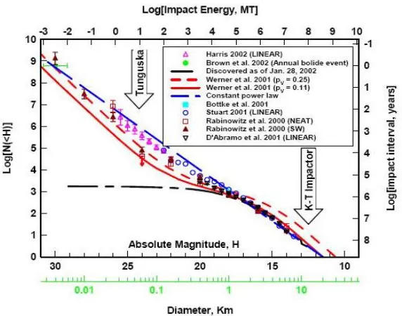
The near Earth asteroid population used is taken from the Near-Earth Object Science Definition report6. It is based on the results of a substantial number of studies estimating the population of different ranges of object sizes by a number of techniques (see Figure 1 taken from Stokeset al.6). The Near-Earth Object Science Definition report provides an accumulative population of asteroids that can be expressed as a constant power law distribution function of object diameter as:
( [ ]) b
N D km CD (1)
Figure 1.Accumulative size distribution of Near Earth Objects (from Stokeset al.6).
Assuming a population of asteroids defined by a power law distribution such as Eq.(1), one can easily calculate the total number of objects within an upper and lower diameter:
min max
min max
b b
N D D D C D D (2)
where Dmax and Dmin are the maximum and minimum diameter chosen. An estimation of the total asteroid mass composed by all these objects can also be computed. To do so, the following integration needs to be performed:
min max min
max
[ ] [ ]
D
D
N
N
D D D km
M
m dN
(3)where m is the mass of the asteroid and
min
D
N and
max
D
N are the number of objects bigger than Dmin and Dmax respectively.
Assuming that all asteroids have a spherical shape and an average density
a, the mass m of the asteroid can bedefined by
6
aD3 and the integration can be defined as an integration over the asteroid diameter:min max min
max 3
[ ] 6 a
D D D
D
dN
D dD
dD
M
(4)where dN dD is the derivative of Eq. (1) with respect D. Integrating Eq. (4), the total mass of asteroid material composed of asteroids with diameters between Dmax and Dmin results in:
max min
3 3
max min
[ ] 6 3
b b
a
D D
C b D D
b
M
(5)The average asteroid density
acan be approximated as 2600 kg/m3
B. Near Earth Asteroid Orbital Distribution
The present section describes the NEA orbital distribution model used to estimate the likelihood of finding an asteroid within a given volume of Keplerian space
a, e, i, ,
, M
. This likelihood can also be interpreted as the fraction of asteroids within the specified region of the Keplerian space, and thus, if multiplied by Eq.(5), results in the portion of asteroid mass within that region. Hence, the ability of calculating this likelihood, together with the ability of defining the regions of the Keplerian space from which the Earth can be reached with a given ∆v budget, will later allow us to compute the asteroid resources available in the near-Earth space.The NEA orbital distribution used here is based on an interpolation from the theoretical distribution model published in Bottke et al.7. The data used was very kindly provided by W.F. Bottke (personal communication, 2009). Bottke et al.7 built an orbital distribution of NEA by propagating in time thousands of test bodies initially located at all the main source regions of asteroids (i.e., the ν6 resonance, intermediate source Mars-crossers, the 3:1 resonance, the outer main belt, and the transneptunian disk). By using the set of asteroids discovered by Spacewatch at the time, the relative importance of the different asteroid sources could be best-fitted. This procedure yielded a steady state population of near Earth objects from which an orbital distribution as a function of semi-major axis a, eccentricity e and inclination i can be interpolated numerically.
The remaining three Keplerian elements, the right ascension of the ascending node Ω, the argument of periapsis ω and the mean anomaly M, are assumed here uniformly distributed random variables. The ascending node Ω and the argument of periapsis ω are generally believed to be uniformly distributed in near Earth orbital space11 as a consequence of the fact that the period of the secular evolution of these two angles is expected to be much shorter than the life-span of a near Earth object12. Therefore, we can assume that any value of Ω and ω is equally possible for any NEA. All values of mean anomaly M are also assumed to be equally possible, and thus M is also uniformly distributed between 0 to 2π.
A probability density function
a e i, ,
has been created by linearly interpolating a 3-dimensional set of data containing the probability density at semi-major axis ranging from 0.05 to 7.35 AU with a partition step size of 0.1 AU, eccentricity ranging from 0.025 to 0.975 with a partition step of 0.05 and inclination ranging from 2.5 to 87.5 deg with a partition step of 5 deg. When
a e i, ,
requires a value outside the given grid of points (e.g., inclination less than 2.5 degrees) then a nearest neighbor extrapolation is used for the dependence in semi-major axis and eccentricity, while a linear extrapolation is used for the dependence in inclination. Figure 2 shows both the
a e i, ,
[image:5.612.101.517.431.665.2] projected in the {a,e} plane and the Aten, Apollo and Amor regions.
Finally, an integration such as:
max max max min min min
, ,
a e i
a e i
P
a e i di de da (6)yields the probability to find an asteroid within the Keplerian elements defined by [amax,amin], [emax,emin] and max min
[i ,i ]. Section III will later describe how these limits can be defined as a function of the delta-velocity budget for different transfer types. The integration of a region of the Keplerian space, by means of Eq.(6), and multiplying this result by Eq.(2) provides a good estimation of the number of objects with diameters between [Dmax,Dmin] that should be found within that region:
expected min, max , min, max , min,max min max
N P a a e e i i N D DD (7)
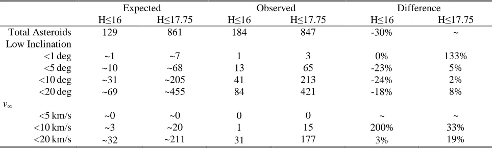
[image:6.612.66.548.390.536.2]When Bottke et al.7 model was under development only 1000 near Earth objects were known, by 15th April 2010, about 7000 objects have been surveyed. The NEA distribution model can then be tested by comparing the prediction of Eq.(7) against the real population. When doing so, care must be taken in comparing our expected population only with the fraction of the surveyed population that is complete or almost completed. The census of small asteroids (< 1km), which is not completed yet, suffers from observational effects (i.e., objects in orbits that can be more easily spotted are first discovered), and this implies that only the census of objects that are almost completed should be compared with the NEA distribution model. Eq.(1) foresees 861 objects bigger than 1 km diameter, currently there are 847 known objects with H≤17.75, i.e., mean absolute magnitude of objects larger than 1km diameter. We then regard the survey of objects larger than 1 km diameter as almost finished, and therefore with little observation bias. Table 1 compares the observed population of asteroids with the expected population of NEA, calculated by means of Eq.(7). The table shows some difference in each one of the Keplerian regions checked, but in general the expected population matches pretty well the observed NEA and the differences can be regarded as statistical deviations from the mean.
Table 1. Comparison between NEA model predictions and surveyed population of asteroids larger than 1 km
Expected Observed Difference
H≤16 H≤17.75 H≤16 H≤17.75 H≤16 H≤17.75
Total Asteroids 129 861 184 847 -30% ~
Low Inclination
<1deg ~1 ~7 1 3 0% 133%
<5deg ~10 ~68 13 65 -23% 5%
<10deg ~31 ~205 41 213 -24% 2%
<20deg ~69 ~455 84 421 -18% 8%
v∞
<5km/s ~0 ~0 0 0 ~ ~
<10km/s ~3 ~20 1 15 200% 33%
<20km/s ~32 ~211 31 177 3% 19%
III.
Asteroid Material Transfer
This section will now describe the methodology followed to map the volume of Keplerian space where capture of asteroid resources is deemed feasible. This is the final element, which together with the NEO model described in section II, provides the means to calculate the available asteroid mass for resource exploitation in the near-Earth orbital space. Several transfer types will be considered here, all of them using multi-impulsive trajectories.
We can also consider the possibility of a single-impulse capture. Even if the asteroid and the Earth have no coplanar motion, asteroid capture would be possible in one single burn if the geometry of the orbits is such that the asteroid‟s MOID is smaller than the sphere of influence of the Earth. If this geometry occurs one single maneuver provided at the perigee passage may suffice to capture the asteroid in an Earth-bound orbit. Finally, a three-impulse transfer will also be described. This type of transfer provides access to resources in the non-Earth-crossing Keplerian region and, at the same time, can reduce the v capture requirement of Earth crossing asteroids. The latter type of maneuver is generally refer as delta-velocity-v∞ leveraging transfer8.
All these transfer models will be described as phase-free transfers. This means that the real orbital position is not taken into account, but only the geometry of the orbits is considered. Clearly, in order for an asteroid to meet the Earth during its orbital motion, not only the MOID must be very small (i.e., geometric consideration), but also the position of the Earth and the asteroid inside their mutual orbits must be very precise. Thus, an additional maneuver will be considered in order to provide the gentle push necessary to render the required phasing at the MOID.
A. Two-impulses method
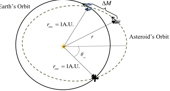
[image:7.612.179.459.293.444.2]On this model and in any other transfer model in the paper, it will be assumed that the motion of the asteroid, or any material resources extracted, is dominated by the gravitational influence of the Sun. The Earth is assumed to be in a circular orbit with radius 1 AU. When the asteroid has a close encounter with the Earth, the motion will be dominated by the Earth‟s influence in a patched-conic approximation.
Figure 3. Orbital geometry of the coplanar model.
As shown in Figure 3, an Earth-crossing coplanar asteroid has two intersections (points of MOID equal 0) with the Earth‟s orbit. These are found when the asteroid is at 1AU from the Sun. Since the distance r from the Sun to the asteroid is known, the equation of the orbit in polar coordinates yields the true anomaly of the two encounters θenc:
1
1
cos
enc
p
e
(8)where 2
(1 )
pa e is the asteroid‟s semi-latus rectum and the unit length in Eq.(8), and any of the following formulas in this paper, has been normalized to 1AU.
With the true anomaly of the encounter θenc known, the velocity at the encounter can now be defined by using
normal and radial components of a Keplerian orbital motion:
sin
enc Sun
r enc
v
e
p
(9)
1
cos
enc Sun
n enc
v
e
p
(10)where vrenc and enc n
v are the radial and normal velocity at the MOID point. Using Eq. (8) and Eqs.(9)-(10), the encounter velocity can be rewritten in a more suitable form:
Asteroid‟s Orbit
1A.U. enc
r
Earth‟s Orbit M
1A.U. enc
r
r
enc
2 2
1
enc Sun
r
v
e
p
p
(11)enc
n Sun
v
p
(12)Whenever the Earth-coplanar asteroid meets the Earth at θenc, the velocity of the asteroid relative to the Earth
will then be
enc,
enc
r n enc
v v r with the Earth moving at an angular velocity:
3
Sun
a
or
Sun sincea
1
AU (13)1. Change of Plane
The first impulsive maneuver in this capture sequence provides the change of plane necessary to make the asteroid orbit coplanar with the Earth. Using a more complex and realistic sequence of maneuvers, a single combined maneuver could provide both the required phasing and the change of plane such that an Earth flyby occurs. In that case, the asteroid transfer to Earth would not need to be strictly coplanar with the Earth and the change of velocity necessary for the maneuver would be minimized. Unfortunately, this procedure would require a full numerical optimization for each individual case, which would be unmanageable for the scope of this paper.
A simpler approach is to consider a change of plane maneuver such as:
2 sin( )
2
inc plX
i
v v
(14)
where vincis the impulsive change of velocity necessary to change the orbital plane by ∆i, and vplXis the velocity of the asteroid at the Earth orbit plane crossing. Equation (14) allows a more analytical approach to the problem and at the same time provides a worst case scenario for the cost of the change of plane.
The velocity of the asteroid at the Earth crossing plane vplXwill vary with the geometry and orientation of the asteroid orbit, i.e., a and e, and argument of the periapsis ω. As it has been previously discussed, the asteroid population model assumes that the argument of the periapsis ω behaves as a stochastic variable. As a consequence, and since the purpose of this model is to assess the asteroid resources that could be captured at the Earth, vplX is defined as the velocity of the asteroid at its semi-latus rectum p, which again yields the worst case scenario for the change of plane maneuver for each orbital geometry. By doing so, Eq. (14) becomes a function only of the semi-major axis a, eccentricity e and inclination i of the asteroid and can be written as:
2
2 1 sin( )
2
Sun inc
i
v e
p
(15) 2. Final Earth Insertion
If MOID is zero or almost zero, the Earth encounter could be easily tuned by a phasing maneuver so that the altitude during the Earth fly-by is some given minimum distance (chosen here to be 200km) above the Earth‟s surface. At this minimum altitude a final insertion maneuver could be performed. Clearly, for large NEA there would be an issue of impact hazard to be considered, however for smaller bodies this hazard can be mitigated since bodies of tens of meters of diameter should completely ablate in the atmosphere13. Thus, bodies in the order of 10 meters diameter may be considered as perfect targets for first capture demonstrator missions.
A parabolic orbit is assumed here to be the threshold between an Earth-bound orbit and an Earth escape orbit. Hence, the ∆v necessary for an Earth capture vcap at the perigee passage results on:
2
2 2
cap
p p
v v
r r
(16)
where v is the hyperbolic excess velocity and rp is the pericenter altitude. As described at the beginning of section III.A, the hyperbolic excess velocity is defined by the relative Earth encounter velocity
enc,
enc
r n enc
v v r and is therefore:
2
22 2
1 Sun
Sun
v e p p
p
since rencis equal to 1 using distance units in astronomical units. Considering that the Earth angular velocity
isSun
for a circular orbit of radius of 1 AU and using simple arithmetic manipulation, Eq.(17) can be simplified to:
21
3
2
Sun vp
a
(18)which is in fact the Tisserand Criterion for the case of ecliptic orbits and fly-by distance at 1 AU.
3. Keplerian Feasible Regions
Given equations (15) and (16), we can now easily estimate the ∆v budgetnecessary to transfer/capture asteroid material to/at Earth from a given {a,e,i} region, ∆v=∆vinc+∆vcap. These two equations can be rearranged so that they
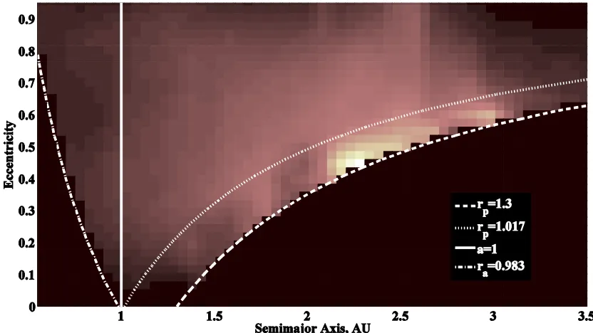
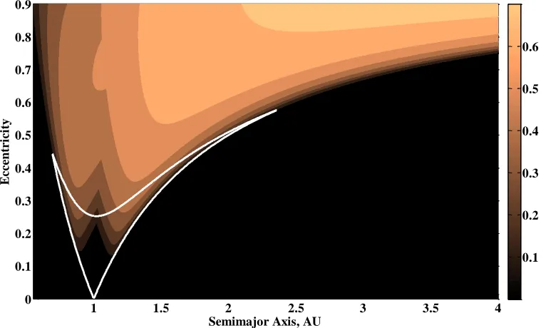
[image:9.612.102.503.270.499.2]yield the Keplerian regions within which capture of asteroid resources is ensured to be bellow a given threshold ∆vthreshold.Figure 4shows the Keplerian region in the plane {a,e} where asteroid resources can be transfer to Earth with a total ∆v equal or lower than 2.37 km/s. This ∆v corresponds to the Moon‟s escape velocity, thus offering a direct comparison between material available at the Moon and within an equivalent energy threshold elsewhere in the solar system. Also, superimposed in the figure are almost 5,000 asteroids (tiny dots and small crosses), which had been surveyed by April 2010.
Figure 4shows three different lines (solid, dash-dotted and dotted line) delimiting an area in the {a,e} plane. The solid line results from expressing Eq.(16) as an explicit function of the semi-major axis a and vcap necessary for an Earth capture:
2 21 1
, 1 3
4
cap
sun
v e v a
a a
where
2
2 2 2
p p
cap
v
r r
v
(19)Equation (19) therefore yields the value of eccentricity for which an asteroid with semi-major axis a can be captured with a maneuver ∆vcap at the perigee passage. Asteroids with semi-major axis a, but eccentricity lower
than the result provided by Eq.(19) should be captured with a maneuver lower than vcap. Thus, if vcapis set to the maximum allowed maneuvervthreshold, the eccentricity resulting from Eq. (19) is also the maximum allowed eccentricity, emax e
vthreshold,a
.Eccentricities lower than emax require lower ∆v maneuvers to be captured at the Earth, but there is a geometrical limit to the minimum Earth insertion maneuvervcap.The minimum vcap occurs when the encounter geometry is
-1.5 -1 -0.5 0 0.5 1 -1 -0.8 -0.6 -0.4 -0.2 0 0.2 0.4 0.6 0.8 1 x y
-4 -3.5 -3 -2.5 -2 -1.5 -1 -0.5 0 0.5 1 -2 -1.5 -1 -0.5 0 0.5 1 1.5 2 x y
max , threshold
e a v
min
e a
-1 -0.8 -0.6 -0.4 -0.2 0 0.2 0.4 0.6 0.8 1 -1 -0.8 -0.6 -0.4 -0.2 0 0.2 0.4 0.6 0.8 1 x y
Figure 4. Keplerian {a,e} space reached by a maneuver of 2.37 km/s (i.e., Moon’s escape velocity).
such that the intersection is at the line of apsis. With this geometry only one intersection point exists, and lower eccentricities imply orbits with no Earth crossing points (see Figure 4). The minimum allowed eccentricity for an orbit with semi-major axis a is therefore:
min
1 1 if 1
1 1 if 1
a a
e a
a a
(20)
so that, if a1,the periapis radius is 1 (see dotted line in Figure 4), and, if instead a1,the apoapsis is 1 (see dash-dotted line in Figure 4).
Once the analytical expressions for the maximum and minimum eccentricity emax and emin are known, the
maximum and minimum allowed semi-major axis a can be computed by finding when emax
v
threshold,
a
emin
a
occurs. The latter equation results in a second degree polynomial with the following two solutions:
min
2 2
1
1 2
threshold
s s
a v
v v
or max
2 2
1
1 2
threshold
s s
a v
v v
(21)
where v2 is defined as in Eq.(19).
Inside this delimited area within the {a,e} Keplerian space, we can ensure that the coplanar capture maneuvers will be lower than the limit threshold. Thus, the reminder impulse, ∆v=∆vthreshold-∆vcap(a,e), can be used for
changing the plane of any available objects as described in section III.A.1. Rearranging Eq.(15), the maximum object‟s inclination that can be modified and set into a coplanar motion with the Earth results:
1
max 1/ 2
2 ,
, , 2 sin
2 1
threshold cap
threshold
Sun
v v a e
i a e v
e p
(22)
Finally, any object within the Keplerian volume defined by equations (19) to (22) will require a total ∆v lower than the limit threshold and some ∆v budget will still be available for phasing. Note that two types of symbols were used in Figure 4 to represent the surveyed asteroids. The small crosses represent all those objects that fall inside the volume calculated by the limits previously described when the Moon‟s escape velocity is used as ∆vthreshold. Thus,
dots falling inside the area delimited in Figure 4 have inclinations larger than the result of equation (22). As shown in the figure, a considerable number of surveyed objects have orbits from which material could be transferred to the Earth with a lower energy requirement than from the surface of the Moon. It is also important to remark that by April 2010 only the survey of objects larger than 1 km diameter is virtually completed, while less than 0.1% of the objects between 30 and 300 meters are known. Hence, an important portion of objects are still to be discovered.
B. One-impulse method
Figure 5. Representation of all possible orientations of an orbit as a function of argument of the periapsis ω.
The figure shows two orbital planes, one for the Earth orbit and one for the asteroid orbit. By continuously changing the argument of the periapsis, all possible orientations of the asteroid orbit in the plane are yielded. The two crosses mark the Earth orbital crossing points which are possible only for four different values of the argument of the periapsis ω. Two arrows show the argument of the periapsis ω for one of the four configurations.
As shown by Figure 5, only 4 specific values of ω yield a MOID equal to zero (i.e., an intersection between the two orbits). Except if the semilatus rectum p is equal to 1, in which case there will be only two values of ω yielding two simultaneous crossing points. Equation (8) already provided the two possible true anomalies that give the asteroid a distance of 1AU from the Sun. Therefore, for the orbital intersection to occur in the non-ecliptic asteroid case, one of these two angles is required to coincide with the line of nodes, i.e., the straight line where the two orbital planes meet. This yields four different arguments of the periapsis ω for which the MOID is 0:
0
MOID enc enc enc enc
i
ˆ
x
ˆ y
x f
[image:12.612.88.554.75.280.2]O
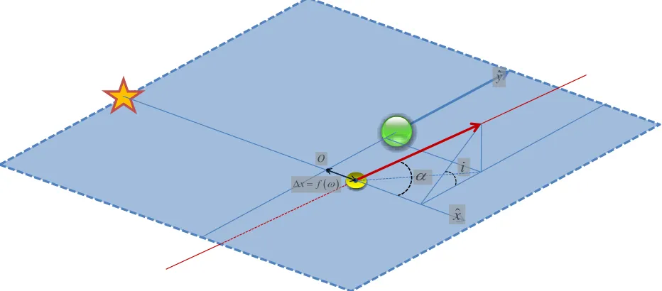
Figure 6. Set of coordinates used to compute Eq.(24).
Close to the values of ωMOID0, the variation of MOID as a function of periapsis argument can be approximated linearly12, 14. With the axis shown in Figure 6, the motion of the Earth and the asteroid can be well described using a linear approximation of the Keplerian velocities of the two objects for true anomaly θenc. This defines two straight
line trajectories, and thus, the minimum distance between these two linear trajectories can be found. The minimum distance can then be written as an explicit function of ∆x (i.e., distance between the centre of the coordinates described in Figure 6 and the point at which the asteroid crosses the Earth orbital plane), which can also be described as a linear function of the argument of the periapsis ω. Finally, an expression such as:
0 2
2 min
1
tan sin
MOID
MOID
i
(24)
yields an approximate value of the MOID distance. The expression min[|.|] denotes the minimum value of the absolute differences with any of the angles ωMOID0 and the tangent of the flight path angle can be calculated as:
2 2tan
1 p
e p
(25)
For a complete derivation of a similar formulae, the reader can refer to Opik‟s work12 or alternatively to Bonanno‟s work14
0 50 100 150 200 250 300 350 10-3
10-2 10-1 100
Argument of the Periapsis, deg
M
O
ID
,
A
U
0 50 100 150 200 250 300 350 10
-2
10-1 100 101 102
D
if
fe
r
e
n
c
e
,%
Difference between numerically and analitically calculated MOID
Numerical MOID
[image:13.612.128.500.73.324.2]Linearly Approximated MOID PHA MOID threshold
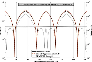
Figure 7. Comparison between the analytical and numerical approaches to compute MOID.
1. Capture at MOID point
Once it has been shown that the analytical approximation of MOID is a reliable way of assessing the distance between two orbits, we can define the maximum MOID at which the capture of an object is possible given a limiting ∆v budget. Eq.(16), in section III.A.2, defined the required Earth capture maneuver vcap as a function of the
hyperbolic excess velocity v∞ andthe pericenter altitude rp. The latter can also be expressed as an explicit function
of the hyperbolic velocity v∞ and the impulsive maneuver:
2 2
2 2
8 cap
p
cap
v r
v v
(26)
Since equation (26) refers to non-coplanar asteroids, the hyperbolic velocity v∞ needs to be calculated as:
2 1
3 2
cos
Sun
v p
a
i
(27)This expression can be derived by noticing that the relative velocity at the encounter for a non-coplanar asteroid can be expressed as
vrenc,vnenccos
i renc,vnencsin
i
.Finally, in order to know the maximum MOID at which a direct capture is possible, the distance rp needs to be
corrected by the hyperbolic factor, i.e., factor that accounts for the gravitational pull of the Earth during the asteroid‟s final approach to the Earth. This results on:
2
MOIDcap p 1
p
r
r v
(28)
Note that if the perigee altitude resultant from Eq.(26) is smaller than the radius of the Earth would mean that the capture of that particular body is not feasible under that particular ∆v threshold used. In fact, the feasible limit for a fly-by was set to 200km altitude from the surface of the Earth, also to account for the Earth atmosphere.
2. Fraction of capturable asteroids
The previous section provided the means of calculating the MOID at which capture is possible as a function of
cap v
2 2 1
MOID tan
sin
cap
i
(29)
a direct capture of the asteroid is possible, since the minimum orbital distance is ensured to be smaller than MOIDcap, and thus, the capture impulse should be smaller than vcap. One may think then that the total range at the
neighborhood of ωMOID0 is 2∆ω, and since there are 4 different ωMOID0, the total range of ω at which capture is possible should be 8∆ω. This is generally correct, but attention must be pay when overlapping of ranges occurs. If the semilatus rectum p is close two 1, the values θenc and π- θenc are also close and their ranges (θenc±∆ω and
π-θenc±∆ω) may overlap, a correction is applied in those cases.
The fraction of asteroids with given {a,e,i} that can be captured with a given ∆v budget is then:
, ,
8
, ,
2 a e i
f a e i
(30)
without overlap correction. Fraction f provides the portion of material with Keplerian elements {a,e,i} that could be capture with a single maneuver (≤∆vcap) at the Earth. Capture of asteroid material by means of only one impulse would simplify considerably the engineering challenges of implementing the two-impulse transfer, described in section III.A, since this type of transfer requires of a spacecraft to be sent to deep-space to perform a change of plane.
3. Keplerian Feasible Regions
The capture feasible regions using one-impulse transfers in the {a,e} subspace are the same than in section III.A.3. The only difference between the feasible volume {a,e,i} of the two-impulse and the one-impulse model lies in the inclination dimension. Since no change of inclination is required, the maximum inclination from which asteroids can be captured is greatly increased. The limit threshold can be computed by realizing that 2
v calculated as in Eq.(27) must be equal to v2 calculated as in Eq.(19), thus:
1 2max
1 1
, , cos 3
2 sun
v
i a e v
a
p
where
2
2 2 2
p p
v
r r
v
(31)
where rp r+200km is the lower limit for an Earth flyby.Note that, unlike the two-impulse transfer model, the
single-impulse transfer is not able to capture all the mass inside the capture feasible region, but only a fraction f (Eq.(30)) of the total mass.
C. Three-impulse method
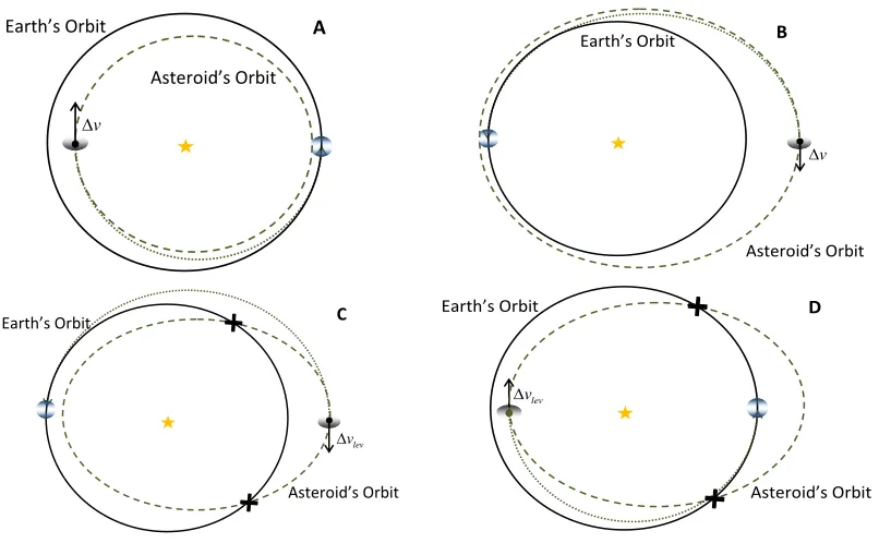
Important enhancement of the accessible Keplerian space can be achieved by adding a further maneuver to the set of impulses described as a two-impulse transfer in Section III.A (i.e., change of plane and Earth capture). Figure 8 show the four cases for which three-impulse transfers are advantageous. Clearly, if more complex transfers are considered, the population of non-Earth crossing asteroids can now be accessed for exploitation, in particular Interior-to-Earth-orbit asteroids (IEOs) and Amor class asteroids could potentially be captured. Also, for asteroids that are already Earth-crossing, a small intermediate maneuver may reduce the necessary ∆v at the Earth orbital insertion.
v
Asteroid’s Orbit
Earth’s Orbit A
v
Asteroid’s Orbit
Earth’s Orbit B
Asteroid’s Orbit Earth’s Orbit
lev
v
C Earth’s Orbit D
Asteroid’s Orbit lev
v
Figure 8. Orbital geometry of Earth transfers and the v∞-leveraging maneuver. Figure A and B show the
Earth transfer for Interior-to-Earth-orbit asteroids (IEO) and Amor class asteroids respectively. Figure C and D show an external and internal v∞-leveraging maneuver, respectively.
Looking at Eq.(16) one can see that the lower the relative velocity at encounter v, the lower the impulse
required for Earth capture. We can also reckon by looking at Eq.(18) that for a fixed semimajor axis, the lower would be the eccentricity, the lower also the relative velocity. If the eccentricity is too low no intersection with the Earth orbit exists, thus the optimal encounter geometry will always be at the line of apsides of the asteroid. Hence, if IEOs or Amor asteroids are transfer to the Earth, the optimal transfer should be such that the encounter occurs at the aphelion or perihelion respectively, and the transfer impulse should then be located at the opposite apsidal point (see Figure 3-A and 3-B). Equation (32) computes the transfer ∆v by comparing the vis-viva equation of the instant before and after the impulse for both transfer types, i.e., A and B.
Amor Type IEO
1
1 2
man a
a trans
r r a e
r a
1
1 2
man p
p trans
r r a e
r a
2 1 2 1
trans sun
man trans man
v
r a r a
(32)
Similarly for Earth-crossing asteroids, the optimal point to provide an impulse maneuver that changes the asteroid relative velocity at Earth encounter is also one of the apsidal points. Thus, the v∞-leveraging maneuver can be completely defined by the distance from the sun of the apsidal point where the maneuver is applied (ra or rp), the
[image:15.612.105.508.71.320.2]Apohelion maneuver Perihelion maneuver
2 1 cos2 1 cos
man a
a trans
trans
a a enc
trans a enc r r r e a r r a r
2 1 cos2 1 cos
man p
p trans
trans
p p enc
trans p enc r r r e a r r a r
2 1 2 1
lev sun
man trans man
v
r a r a
(33)
[image:16.612.133.527.73.192.2]Equation (33), together with Eq.(16), can be optimized to find the optimal encounter angle θenc that minimizes the most the cost of the coplanar maneuvers ∆vlev+∆vcap. The result of the optimization shows that whenever the v∞ -leveraging strategy is able to reduce the cost of the capture, then the optimal encounter angle θenc is always one of the apsidal points (either π or 0 rads). There is also a region for which the v∞-leveraging is not providing any improvement to the total capture ∆v budget. Figure 9 shows the regions in the Keplerian plane {a,e} in which the v∞-leveraging strategy is advantageous, as well as the approximate reduction factor of ∆vlev+∆vcap versus a single ∆vcap. Also the area of feasible capture for a two-impulse transfer and ∆vthreshold of 2.37km/s is superposed in the
figure for comparison purposes.
1 1.5 2 2.5 3 3.5 4
0 0.1 0.2 0.3 0.4 0.5 0.6 0.7 0.8 0.9
Semimajor Axis, AU
Eccentri ci ty 0.1 0.2 0.3 0.4 0.5 0.6
Figure 9. {a,e} regions where v∞-leveraging strategy is of advantage for coplanar Earth-crosser asteroids. The color scale shows the fraction of ∆v saving. Also superposed in the figure is the feasible capture region for a
two-impulse transfer with ∆vthreshold of 2.37km/s.
4. Keplerian Feasible Regions
[image:16.612.124.507.309.539.2]transfer to Earth orbit with energy lower than the required to escape the Moon‟s gravity well, Figure 10 shows a total of 214 asteroids.
Figure 10. Three-impulse transfer Keplerian {a,e} space reached by a maneuver of 2.37 km/s (i.e., Moon’s escape velocity). Superimposed are all near Earth asteroids known within the {a,e} space as of April 2010.
D. Phasing maneuver
Previous sections have assumed that if the orbital intersection existed, then the asteroid would eventually meet the Earth. This statement may be true if the time available to transfer the asteroid is not constrained, but for realistic scenarios this does not occur. Therefore, some analysis on the cost of the maneuvering necessary to ensure the encounter opportunity must be performed.
Thus for a more realistic transfer scenario, in which the orbital phasing is also considered, an additional impulsive maneuver may be necessary in order to provide the right phasing to the asteroid. This maneuver is generally small and must be provided as early as possible, so that the secular effect due to the change in period yields the orbital drift necessary for the asteroid to be at the Earth orbital crossing point at the required time. Hence, if only secular effects are considered15-16, which is regarded as a good approximation for the level of accuracy intended in this paper, the phasing maneuver should correct the difference in mean anomaly ∆M that exists for the intended encounter (see Figure 3). This is expressed as:
M n t
etm
(34)where ∆n is the change of mean motion of the asteroid due to the phasing maneuver and (te-tm) is the time-span
between the maneuver (tm) and the encounter (i.e. time at which the Earth is at the crossing point te). The change in
mean motion of the asteroid can be defined as:
3 3Sun Sun
n
a
a a
(35)
where δa is the change of semi-major axis of the asteroid due to the impulsive maneuver. Using the Gauss planetary equations17, δa can be expressed as:
0
2 2
t Sun
a v
a v
(36)
where δvt is the tangential component of the impulsive maneuverand v0 is the orbital velocity at the point at which
the impulsive maneuver is applied. Eq.(36) seems to indicate that the optimal position for a phasing maneuver is the periapsis, since this is the point at which the orbital velocity v0 is maximum. This is generally true, except for cases
in which the term (te-tm) of equation (34) drives the optimality of the phasing maneuver.
0
1 3
2 2
3
2
Sun Sun
t
Sun e m
v a
a v M
t t a
(37)
which provides a good estimation of the cost of the encounter. Note that this implies that the optimal phasing maneuver has only tangential impulse.
Considering an Earth-asteroid configuration such as in Figure 3, an algorithm was implemented that computes the fraction of mean anomalies inside the asteroid orbital path that can be phased with the Earth with a δvt smaller
than a given threshold. The algorithm requires as an input the ∆M at a given time te at which the Earth is assumed to
be in the crossing point from which ∆M is measured. Also a time constraint needs to be specified, which defines the maximum allowed maneuver time tmaxm. Then, the algorithm computes the δvt necessary to cancel not only the ∆M
gap at time te, but also all other possible encounters opportunities, which are defined by the times at which the Earth
is at the crossing points during the time-span available. For each possible encounter two maneuver times are considered; the first available periapsis passage and the tmaxm. This procedure is repeated for thousand different
angular positions ∆M at te, from which then the fraction of the orbit that can be phased under a ∆v limit is calculated.
IV.
Asteroid Exploitable Mass
Transfers and asteroid population model can finally be set together in order to estimate the available material that could be exploited by future space missions. The total available material will be mapped as a function of the limiting ∆v budget, and as described in section III, once a ∆v threshold has been fixed, the Keplerian regions of feasible capture can be calculated for each transfer type. These regions delimit the set of {a,e,i} from which an asteroid could be transported to a weakly-bound Earth orbit with a transfer requiring a total ∆v lower than a fixed threshold. The fraction of the near-Earth object population that falls into this feasible region can be calculated by integrating Eq.(6) over the entire feasible volume. The integration limits of Eq.(6) were defined for each particular transfer model as functions of ∆vthreshold, semi-major axis a and eccentricity e:
min max
min max
min max
, ,
, , , ,
threshold threshold threshold threshold
threshold threshold
a v a a v
e a v e e a v
i a e v i i a e v
For the free-phase two-impulse and three-impulse transfer, any asteroid within the feasible capture region could, in principle, be capture (or its material exploited). On the other hand, the one-impulse is a special case in which only a fraction f (see Eq.(30)) of asteroids at each {a,e,i} point will have the conditions necessary to ensure a capture bellow the ∆v threshold. Thus, in this case, the integration required is:
max max max min min min
, , , ,
a e i
a e i
P
a e i f a e i di de da (38)When P is known, the total mass of near Earth objects is calculated by means of Eq.(5), where a range of diameters need to be specified. By multiplying the probability P by this total mass of NEA within the given range of object size, one obtains the total asteroid mass that could be theoretically captured and exploited given a ∆v budget.
[image:18.612.226.392.73.144.2]A. Total Available Mass
10-3 10-2 10-1 100 106
108 1010 1012 1014
V
threshold, km/s
To
ta
l
C
a
ptured
M
a
ss
,
kg
[image:19.612.78.505.78.347.2]One-impulse Transfers Two-impulse Transfers Three-impulses Transfers
Figure 11. Total asteroid mass available for exploitation of resources as a function of ∆v threshold.
A comparison can now be made of the exploitation of lunar and asteroid resources. Figure 11 shows that for avthreshold equal to the Moon‟s escape velocity (i.e., 2.37 km/s) the total available asteroid material is 2.4x10¹² kg if only one maneuver is considered, 1.1x10¹³ kg for two-impulse transfers and 6.3x10¹³ kg with three impulses. In addition to the fact that the Moon is believed to be a very resource-poor body18, lunar resources would require a minimum v of 2.37 km/s to be extracted from the lunar gravity well. However, as shown in Figure 11, an important aspect of asteroid resources is that they can be exploited at a whole spectrum of v. For example, for a vthresholdof 100 m/s a total mass of 6x10⁹ kg could be transferred to Earth by using a one-impulse transfer. Considering, for example, that about 10% of objects are expected to be hydrated carbonaceous asteroids19, and that those are believed to have contents of water around 8.5% of the weight of the asteroid18, this 6x10⁹ kg of material represent, among others exploitable resources, about 25,000 tons of water. All this water should be concentrated in a few of the largest asteroids within the “reachable” region, since in a power law distributed population most of the mass is carried by the largest objects. Note also, that the energetic cost of shipping these 25,000 tons of water to low-Earth Orbit (e.g., 200 km circular orbit) would be 2.7 times lower than shipping the same the water from the Earth surface. In fact, there should be a total of 4x10¹⁰ tons of water available in near-Earth orbit that could be used in LEO at a lower cost than water from the surface of the Earth.
The transfers models used in this paper provide a conservative scenario for the required v and so the available asteroid mass found is then a low estimate. More complex trajectories, such as multiple Earth fly-by, lunar gravity assists or manifold dynamics20, would be expected to provide a significant increase in captured mass. Note that if an optimized trajectory reduces v cost in, for example, 33%, the total available mass is increased by a much higher proportion. For example of 100 m/s threshold, a 33% reduction in v will allow access to the regions reached by 150 m/s transfers, which would yield 1.2x10¹⁰kg of mass to be captured, hence a 100% increase.
B. Maximum and Time Constrained Mass
As it has been previously remarked, all transfers model were assumed phase free. Thus, it remains to analyze the effects of inducing a correct phasing to asteroid in order to meet the Earth at the orbital crossing points (see Section III.D.). The results shown in Figure 11 assumed that the time available for transferring the asteroid material is sufficiently large so that the phasing maneuver required is negligible, but a more realistic scenario should also considered a maximum time allowed for the transfers described throughout Section III.
In order to include the effects of phasing maneuvers, the integration in Eq.(6) needs now to include a new term to account for the fraction of asteroids that can be phased with the Earth with a ∆v maneuver lower than the remaining delta-velocity. This remaining ∆v is, at each {a,e,i} point in the Keplerian space, the difference between the ∆v required for a capture and the given ∆vthreshold.
max max max min min min
, , ( , , ), , ,
transfer
a e i
t a e i threshold transfer transfer
P
h a ev v a e i t a e i di de da (39)where h is the fraction of material that can be “phased” with a ∆v lower that the remaining ∆v budget, i.e., ( , , )
threshold transfer
v v a e i
, vtransfer( , , )a e i refers to the cost of the nominal transfer as described in section III and ∆ttransfer is the limiting time-span for the transfer. A slightly more complicated expression is required to compute
transfer
t
P for the case of one-impulse transfers, since the cost of the nominal transfer also depends on the argument of
the periapsis,vtransfer( , , , )a e i
.Note that, in the one-impulse transfer case, the argument of the periapsis ω defines the altitude of the fly-by, and thus, strongly influences the cost of the Earth orbital insertion, Eq. (16). In this case, to computetransfer
t
P , the expression for f in Eq.(38) should be calculated as:
0
0
4 , , ( , , , ),
, ,
2
MOID
MOID
threshold transfer transfer
h a e v v a e i t d
f a e i
(40)
10-3 10-2 10-1 100
104 106 108 1010 1012 1014
V
threshold, km/s
To
ta
l
C
a
ptured
M
a
ss
,
kg
40 years transfer time 20 years transfer time 10 years transfer time One-Impulse Transfer
[image:20.612.105.535.316.632.2]Two-Impulse Transfer Three-Impulse Transfer
Figure 12. Total captured mass and time constrained exploitable mass.