Wavelet based feature extraction methods for the discrimination and regression of spectral data

Full text

(1)This file is part of the following reference:. Mallet, Yvette Lelia (1997) Wavelet based feature extraction methods for the discrimination and regression of spectral data. PhD thesis, James Coook University. Access to this file is available from: http://eprints.jcu.edu.au/17437.

(2) WAVELET BASED. FEATURE EXTRACTIO'N METHODS FOR THE DISCRIMINATION AND REGRESSION. OF SPECTRAL DATA. Thesis submitted by. Yvette Lelia MALLET ·Bsc(Hons) Qld in October 1997. for the degree of Doctor of Philbsophy. in the School of Computer Science, Mathematics and Physics James Cook University of North Queensland.

(3) IN MEMORY OF" TES EVERIN9HAM".

(4) STATEMENT OF ACCESS. I, the undersigned, the author of this thesis, understand that James Cook University of North Queensland will make it available for use within the University Library and, by microfilm or other means, allow access to users in other approved libraries. All users consulting this thesis. wil~. have to sign the following statement:. In cunsulting this thesis I agree not to copy or closely paraphrase it in whole or in part without the written consent of the author; and to make prope~ public written acknowledgement for any assistance which I have obtained from it. Beyond this, I do not. vvish to place any restriction on access to thIs thesis.. .. III. ?. /z /0\. . ;"";;~.~.~./~. k I. I. (Date). ..

(5) STATEMENT ON SOURCES. DECLARATION. I declare that this thesis is my own work and has not been submitted in any form for. another degree or diploma at any unIversity or other institution of tertiary. educ~tion.. Information derived from the pu.blished or unpublished work of others has been acknowledged in the text and a list of references is given .. ;'-.~;; ~ ~~::',f{~. ··~/···;···i·"·V·······"············. (Date). iv.

(6) ACKN OvVLED G EMENTS. Foremostly, I thank my supervisors A/Prof Danny Coomans and A/Prof Olivier de Vel, for their professionalism and encouragement in the development of this thesis. I am also grateful for the many hours that they have spent revising this and other manuscripts throughout the course of my research work. I extend my appreciation to Professor Massart for allowing me to visit his laboratory at the Free University of Brussels and providing me with the opportunity to become more familiar with NIR data. Also from the Free University, I thank Delphine Jouan-Rimbaud, Paula Fernandez, Eric Bouveresse, Wu. Wen~. Beate Walczak and Wim Penninckx, for their. assistance. Sincere thanks is expressed to Dr. J~roslav Kautsky. at Flinders University in Adelaide,. who gave up his valuable time to introduce me to wavelets. I would also like to thank Dr Bill Moran, Radka Turcajova and Pavel Turcaj for their assistance and cooperation whilst. I was visiting Flinders University. I extend my appreciation, to Professor Trevor Hastie for supplying his S-plus code and providing valuable input. Many people have provided data which I have used as part of my thesis, these people are acknowledged in Sections 7.2 and 8.2 of this thesis. Thanks to my colleagues in the School of Computer Science, Mathematics and Physics at James Cook University for their encouragement during the final stages of this thesis. In particular to Dr Wayne Read for revising parts of this thesis. The encouragement provided by A/Prof Bob Staudte was also much appreciated.. Whilst pursuing the research summarized in this thesis, I was primarily supported by the Australian Government in the form of an Australian Postgraduate Research Avvard.. I wisll to thank my fiance, Andrew Everingham for his continual support and encouragement. I would also like to thank my team-mates for their patience and understanding. Finally, I thank my mother for alV\Tays thinking of the little things that mean so much.. v.

(7) ABSTRACT. This thesis is concerned with the application of statistical methods to spectral data. A major concern which arises from spectral data is that the number of variables or dimensionality usually exceeds the number of available spectra. This leads to a degradation in performance of traditional statistical methods. There are basically two strategies which can be implemented for overcoming such situations. It is common practice to first reduce. the dimensionality of the data by some feature extraction preprocessing method, and then use an appropriate low dimensional statistical procedure. An alternative procedure is to use a high dimensional statistical procedure which is capable of handling a large number of variables. This thesis considers both approaches, and investigates the applicability of wavelets as features for statistical analyses, as well as other feature extraction procedures.. The particular statistical analyses investigated are discriminant and regression analysis. It is shown that, the wavelet based methods, particularly wavelets which have been designed to suit a particular task, perform quite adequately when compared to traditional approaches.. VI.

(8) Contents. 1. 2. Thesis. 1.1. Overview. 1.2. Thesis Structure and Contribution. 1. .. '.. 9. Discriminant Analysis. 12. 2.1. Introduction.. 12. 2.2. Notation . . .. .......... 16. 2.. 3. Fisher's linear Discriminant Analysis (FLDA). 17. 2.4. Flexible Discriminant Analysis (FDA) . .. 19. 2.5. Penalized Discriminant Analysis (PDA) .. 26. 2.6. Bayesian Classifiers . . . . . . . . . . . . .. 27. 2.6.1. Bayesian Linear Discriminant Analysis (BLDA) ... 28. 2.6.2. Bayesian Quadratic Discriminant Analysis (BQDA). 2.7 2.8. 3. 1. SUillll1ary. Regulari 7:8d Discriminant Analysis (RDA). ....... 29 29. Assessment of Model Performance. 31. 2.8.1. Assessment Criteria . . . . .. 31. 2.. 8.2. Choosing the Evaluation Set. 33. Regression Analysis. 37. 3.1. Introduction.. 37. 3.2. Notation ..... 38. 3.. 3 Multiple Linear Regression (MLR). 39. 3.. 4. 40. Principal Component Regression ... vii.

(9) 4. 3~5. Partial Least Squares Regression . e. 40. 3e6. Assessment of Model Performance. 42. 3~6el. Assessment Criteria . . . . e. 42. 3e6e2. Choosing the Evaluation Set. 44. 4el. 4e2. 5. 47. Feature Extraction. 48. Feature Selection 4.1.1. Feature Selection Strategies for Discriminant Analysis. 48. 4ele2. Feature Selection Strategies for Regression Analysis. 50. 4~le3. Classification and Regression Trees (CART) .. 53. Feature Transformation e. ~. ee.. ~. . . . . . . . ... .. 55. 4.2.1. Preprocessing Methods and Transformations. 55. 4.2.2. Principal Component Analysis (peA). 63. 4e2e3. Fourier Transform (FT) . . . e . . .. 4.2.. 4. Discrete Wavelet Transform (DWT). ..... ,.. . 66 67. Wavelets. 70. 5.1 Introduction.. 72 ...... 74. 5.2. Fourier Transform. 5.3. Windowed Fourier Transform. 74. 5e4. Continuous Wavelet Transform. 7.5. 5.5. Discrete Wavelet Transform. 76. 5.6. Multiresolution Analysis . e. 77. 5.7. Fast Wavelet Transform. 81. 5.8. Higher Multiplicity Wavelets. 5.9. The Discrete \iVavelet Transform of Discrete Data ... 84. 5.10 The m-band Discrete Wavelet Transform of Discrete Data. 96. 5ell The m-Band Discrete Wavelet Transform of a Discrete Data Set. 98. 5.12 Filter Coefficient Conditions. 82. ......... 4. •. •. •. • • • • •. viii. ~. • • •. e. • • • • ,.. e. ••. .. 100.

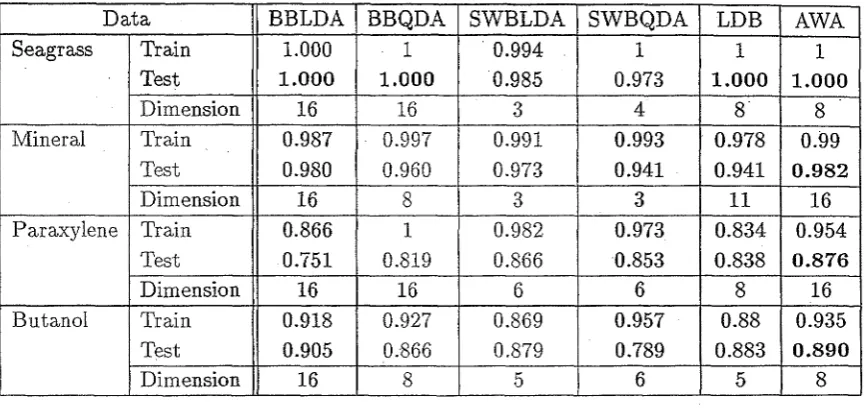
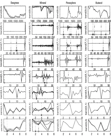
(10) 5.13 Boundary Related Issues . . . . . . . . . . . . . .. ... 102. 5.14 The Wavelet Packet Transform of Discrete Data. · . 103. 5.14.1 The Best Basis Algorithm. .. 5.14.2 The Local Discriminant Basis Algorithm 6. 7. Adaptive Wavelets. . . 105 · . 107 109. 6.1. Introduction.............. ... . . 109. 6.2. Factorization of Wavelet Matrices . . .. · . 110. 6.3. Criteria Measures for Optimization .. . .. 113. 6.3.1. Discriminant Criterion Functions .. . . 113. 6.3.2. Regression Criterion Functions. · . 115. 6.4. The Adaptive Wavelet Algorithm .. 6.5. Example. . 116 . ... 118. .. Classification Applications 7.1. Overview. 7.2. The Data Sets. 121. .... 121. ...... · .122. 7.2.1. Seagrass Data.. . .. 122. 7.2.2. Mineral Data .. · . 123. 7.2.3. Paraxylene Data. · .124. 7.2.4. Butanol Data. . . .. . ....... 7.3. Discriminant Analysis Based on.the Original Variables. 7.4. Discriminant Analysis Based on Wavelet Coefficients. · .125. · . 126 · .. 131. 7.4.1. Exploring. the DWT. 7.4.2. Banded Discriminant Analysis. 7.4.3. Stepwise Feature Extraction from the DWT. · .. 139. 7.4.4. Local Discriminant Bases . .. .... 143. 7.. 4.5. Adaptive \iVavelet Algorithm. 7.4.6. Summary of the vVavelet Feature Extraction Strategies.. .. ix. · . 132 · . 133. . . . . .. · .. 145 . . 151.

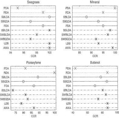
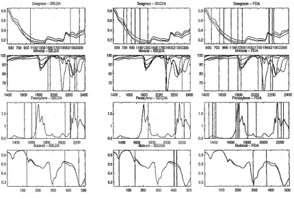
(11) 7.5. 7.6 8. · . 153. 7.5.1. Performance Based Measures. · .154. 7.5.2. l2ualitative Assessment. · . 156. Summary. .. · .168. Regression Applicatio.ns. 170. 8.1. Overview. 8.2. The Data Sets. · . '171. 8.2.1. Sugar Data. · .171. 8.2.2. Wheat Data. .. ..... · . 170. . 172. 8.3. Common Approaches for the Regression of Spectral Data. . 173. 8.4. Regression Analysis Using Features From the DWT. . 176. 8.5. 8.6 9. Which Classification Strategy? . . .. .. .178. 8.4.1. Exploring the DWT. 8.4.2. Banded ¥ultiple Linear Regression (BMLR). .178.. 8.4.3. Stepwise Feature Extraction.. .181. 8.4.4. Adaptive Wavelet Algorithm. 8.4.5. Summary of Wavelet Based Feature Extraction Strategies . . . . . . 187. ... 184. .188. Which Regr,ession Strategy? . . . . . 8.5.1. Performance Based Measures. 8.5.2. Qualitative Assessment. .... 189. .. . 196. Summary . . . . . . . . . . . . . . . . . .. .. 211 213. Concluding Reluarks. . . . 213. 9.1. Original Contribution. 9.2. Summary of Results .. .214. 9.3. Future Work and General Remarks About the AvVA. .217. A. 219. x.

(12) List of Figures spectrun~. obtained from a sample of paraxylene... 2. 1.1. A. 1.2. The electromagnetic spectrum.. 2. 1.3. A discriminant analysis problem.. 3. 1.4 -Feature extraction model. . . .. .5. 1.5. Some wavelet basis functions.. 7. 1.6. Integrated feature extraction model.. 8. 1.7. Thesis outline. .. 9. 2.1. Percentage of correctly classified objects obtained by three dis-. .. criminant techniques (Dl,D2 and D3) for eight combinations of dilnensionality and class sample sizes. . . . . . . . . . ~f. SOlne discriminant analysis methods.. 13. 2. 2. Summary. 2.3. A scatterplot of the discrimi~ant scores produced by FLDA.. 19. 2.4. The FDA algorithm.. 20. 3.1. Partial least squares algorithm.. 4.1. A CART lTIodel. . . . . . . . . . . . . . . . . . . .. 53. 4.2. DelTIOnstration of the SNV transformation. . .. 56. 4. 3. Demonstration of detrending cOlnbined with the SNV transfor-. n1.ation. . . . . . . . . . . . . . . . . . . .. 15. .. . . . . . . . . . .. . ...... 42. 58. DelTIOnstration of the hull quotient .... .59. Demonstration of the second derivative transformation. . .. 60. Xl.

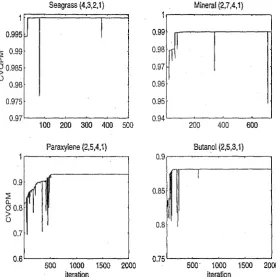
(13) 4.6. A simplified procedure for performing the second derivative trans-. formation. . . . . . . . . . . . . .. . . .. 61. 4.7. Demonstration of mean centering.. 63. 5.1. Fourier -.and wavelet coefficient of a sampled SIne signal, with (right) an.d without (left) a small disturbance. . . . . . . . .. 71. 5.2. SOlne wavelet basis functions from the Daubechies family.. 76. 5.3. Pictorial representation of a 2 band DWT for a signal which has been sampled 8 times. . . . . . . . . .. 90. 5.4. Labelling of the bands in the DWT.. 91. 5.5. 2-bal~d. 92. 5.6. Another presentation for a 2-band DWT perforlned on the gen-. DWT performed on a generated spectrUlTI to level three.. erated spectrum to level three.. . . . . . . . . . .. 93. 5.. 7. Two-band DWT for a spectrum to six levels. .. 95. 5.8. A 3-band discrete wavelet transform. . . . . . .. 97. 5.9. Boxplots obtained from the correlation coefficients discussed for Table 5.1.. . . 100. . . . .. 5.10 Wavelet packet transform with m. = 2.. . .. ~. . . .. . . 104. 5.11 ' Best basis algorithm'. 5.12 Best basis ... ~. . 106. . . . . .. . 107. 6.1. The adaptive wavelet algorithln.. 7.1. Five sample spectra froin the seagrass data.. . . 123. 7.2. Five sample spectra fron'! the Inineral data. . .. . . 124. 7.3. Five sample spectra from the paraxylene data.. . .. 125. 7.4. Five salnple spectra froin the butanol data. . . . . .. . .. 126. 7.5. Correct classification rates (CCR) and quadratic probability mea-. 117. .. sures (QPM) for the seagrass (5), mineral (m), paraxylene (p) and butanol (b) data... . . . . . . . . . . . . . . . . . . . . . . . . . . . . . . . 131 7.6. The DWT and inverse DWT p_erformed on the seagrass ,data. . . . 134. xii.

(14) 7.7. The DWT and inverse DWT performed on the mineral data. . . . 135. 7.8· The DWT and inverse pWT performed on the paraxylene data. . 136 7.9. The DWT and inverse DWT performed on the butanol data. . .. 137. 7.10 Coefficients selected from theDWT by SWBLDA. . . . . . . . 7.11 Selected wavelet coefficients (asterisks) from the best bases.. . 142 . . . 144. 7.12 Discriminant measure versus iteration for the adaptive wavelet. l49. algorithm. 7.13 Correct classification rates (CCR) and quadratic probability measures (QPM) for thp "Wavelet based Inethods applied to the sea-. grass (s), mineral em), paraxylene (p) and butanol (b) data. . . . . 152 7.14 Correct classification rates for each of the discrilninant strategies. 155 7.15. Wavel~ngths. selected by SBLDA, SBQDA and FDA.. . . 158. 7.16 Discriminant plots produced by FDA. . . . . . . . . . . .. . .. 160. 7.17 Coefficients from the DWT which were selected by SWBLDA (asterisk) and SWBQDA (circle). 162. 7.18 Reconstructed spectra produced from the coefficients selected by SWBLDA and SWBQDA. . . . ....... ~. . . . . . . . . . . . . . . . . . .. 163. 7.19 The wavelet coefficients and reconstructed spectra pro.duced from ~. the AWA. .. 165. 7.20 Discriminant plots produced by from the coefficients produced by the AWA. . . . . . . . . . . . . . . . . . .. . .166. 7.21 Discrilninant plots produced by PDA.. . . 167 . .17. 8.. 1. Five salnple spectra frOlTI the sugar data. . ........ 8.2. Five sample spectra from the wheat data... 8.3. Test r-squared values corresponding to the brix, fibre and .proteil~. . 172. responses. . '" . . . . . . . . . . . . . . . . . . . . . . . . . . . . 8.4. The DWT and inverse DWT performed on the sugar data.. 8.5. The DWT and inverse DWT performed on the wheat. 8. 6. Coefficients selected. frOlTI. d~ta.. 175 .. 179 . . 180. the DWT by SMLRW. . . . . . . . . . .. 183. xiii.

(15) 8.7. Regression criterion measure versus iteration for the adaptive. wavelet algorithm.. . . . . . . . 187. 8.8. Test r-squared ,values for the wavelet based regression Inethods. . 189. 8.9. Test 'r-squared values each of the regression strategies.. 189. .. 8.10 Test r-squared values each of the regression strategies (SMLRW and SPCRW not shown). .. . . . . . . . . . . . . . . . . . . ... .. 190. 8.11 Residuals versus fitted values for the brix response models.. . . 194. 8.12 Residuals versus fitted values for the fibre response models.. . . 195. 8.13 Residuals versus fitted values for the protein. respOl~se. models. . . 196. 8.. 14 Histograms of the residuals from the brix response models.. . . 197. 8.15 Histograms of the residuals from the fibre response models.. . . 198,. 8.16 Histograms of the residuals from the protein response models. .. 199 8.17 Plots of the residuals versus the fitted values for each of the lTIod-. els for brix. . . . . . . . .'. . . . . . . . . . . . . . . . . . . .. . . . . . . . 200 8.18 Plots of the resiquals versus the fitted values for each of the mod-. els for fibre. . . . .. '. . . . . . . . . . . . . . . . . . . . . . . . . . . . . . 201 8.19 Plots of the residuals versus the fitted values for each of the lTIod-. els for protein. . . . . . . . . . . . . . . . . . . . . . . .. . . 202. 8.20 Wavelengths selected --by SMLR-Sl and SMLR-S2.. . . 203. 8.22 Regression coefficients obtained froln PLS, when the data" has been standardized.. . . . . . . . . . . . . . . . . . . . . . . . . . . . . 203. 8.21 Absolute correlations between each wavelength and the principal components selected by SPCR.. "~ . . .. .. 204. 8.24 Reconstructed spectra produced from the coefficients selected by SMRLW. ~. ~. 8.23 Coefficients frOln the DWT which were selected by SMLRW. 205. 206. 8.25 Reconstructed spectra produced frall1. the coefficients selected by SMRLW that pertain to the same band.. . . . . . . . . . . . . . . . . 208. xiv.

(16) 8.26 The wavelet coefficients and reconstructed spectra produced from. the AWA. 210. xv.

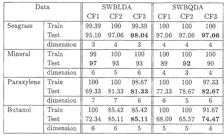
(17) List of Tables 5.1. Summary statistics for the correlation coefficients of the scalin.g. .. and wavelet coefficients of a spectral data set. 6.1. 100. The percentage of correctly classified spectra, uSIng the coefficients {X [3] ( T)} for T == 0, ... , 3 at initialization and at termina-. tion of the adaptive wavelet algorithm. The discriminant criterion functions were Wilk's Lambda, symmetric entropy and the CVQPM. 6.2. . 119. The percentage of correctly classified spectra, using the coeffi-. cients {X[3](r)} for r == 0, ... ,3 at initia.lization and- at termination of the adaptive wavelet algorithm. Optimization was based on {X[3](O)} and the discriminant criterion functions were Wilk's. 120. Lambda, symmetric entropy and the CVQPM.. 7.1. Description of the spectral data sets used for classification.. . 122. 7.2. Correct classification rates (%) for the stepwise procedures.. . 128. 7.3. Original variables selected by SBLDA and SBQDA.. . 129. 7.4. Correct classification· rates (%) .. 7.5-. Quadratic probability measures. . 130. 7.6. Classification results for BBLDA.. .138. 7.7. Classification results for BBQDA. . .. 7.8. Correct classification rates for SWBLDA and SWBQDA.. . .. 130. . .139. .140. 7..9· Coefficients selected by the forward schemes for SWBLDA and. .. SWBQDA.. xvi. 140.

(18) 7.10 Classification performance of the LDB algorithm.. ...... 7.11 Classification results for the adaptive wavelet algorithm.. . 145. . . 148. 7.12 Classification results for the adaptive wavelet algorithm where optimization was over a· scaling and wavelet band for the (4,3,2) setting. . . . . . . . . . . . . . . _" . . . . . . . . . . . . . . . . . . . . . . . 150 7.13 Correct classification rates for the wavelet based feature extrac-. tion strategies. . . . . . . . . . . . . . . . . . . . . . . . . . . . . . . . . . 151 7.14 Quadratic probability measures for the wavelet based feature ex-. 152. traction strategies. 8.1. Description of the spectral data sets used for regression.. 8.2. Training and test R-squared values.. . . 171. .. . .175. 8.3 . Wavelengths selected by the SMLR routines, and the priIlcipal cOlnponents selected by SPCR.. ........ . . 177. 8.4. Classification results for banded BLDA.. . .. 181. 8.5. R-squared values for SMLRW-Sl and SMLRW-S2.. 8.6. Coefficients selected from the DWT by SMLRW-Sl and SMLRW-. 82.. .. . . 182. . . 182. ,........ 8.7. R-squared values for SPCRW-Sl and SPCRW-S2.. 8.8. COlnponents selected from the DWT by SPCRW-Sl and SPCRW82.. 8.9. .o.o.. . ... 184. . • 185. o.......... Regression results for the adaptive wavelet algorithm. .. 8.10 Train.ing and test r-squared values for the.wavelet based approaches. . . . . . . . . . . . . . . . . . . . . . . .. 8.11 Summary of p-values for the regression mOdels. .. XVII. . . 186. regressiol~. . .. 188 . . 192.

(19) List of Symbols Non-bold Lower" Case Letters " a(x) appreciation score of x CD. accr(x) appreciation score equal to 1. if P(r. • aA(x) appreciation score equivalent to P(r. I Xi(r)) 2: P(r I xi)and zero otherwise I Xi(r)). • aQ(x) quadratic appreciation score of x •. ail. CD. a parameter used in RDA which weights· the pooled covariance matrix. Ith element in the ith principal COffiDonent vector. • b parameter used in RDA which controls shrinkage of the weighted pooled covariance matrix • bi ith element in the vector of estimated regression coefficients b " band(j, t) 7th band 7 E {a, 1, ... , m - I} at the jth level j E {J, J - 1, ... , J -. maxlev + I} of the DWT •. Cj,k. scaling coefficients. " dj,k. wavelet coefficients. •. orthogonal projection of'f(t) onto. fVj. Vi. • 9 (x, r) classification score •. gblda(X,. • 9bqda(X,. r) BLDA classification score r) BQDA classification score. • hk high pass filter coefficients o. nii. is the element along the ith diagonal of the hat matrix 1-l. • j* cOlnplex number. A. xviii.

(20) • j parameter controlling the dilation of the wavelet basis functions. • k parameter controlling the translation of the wavelet basis functions • /!,k. low pass· filter coefficients. .. m number of bands in the DWT; downsampling rate • maxlev maximum number of levels in the DWT.. • n number of observational units in the training data set • n' number of observational units in the testing data set. • n r number of observational units from class r; rth element in the vector n number of objects in node 1 of CART model. • n[~. number of levels that an object has been transformed, in the DWT. •. nlevel s. CD. P dimensionality of the data set. • P* dimensionality of the reduced data set P* ~ P. • Po number of parameters to be estimated (including the intercept) in a MLR model. • p(x) is the class probability density of x • q the number of sub-matrices in the filter coefficient matrix A is q + 1 • r index for class categories •. So. minimum of one less than the total number of classes (R-l), or the dimensionality. (p). • s* number of discriminant variables used for assigning an object to a class; s* ::;; •. Xi. •. xi[l]. ith element in the data vector x ith object in node l of CART model. .. Yi ith element in the response vector y • Y~ ith element in the test response vector y'. xix. So.

(21) • YiP] response value of ith ,object in node I of CART model. • Y-i predicted value of Xi, obtained when Xi is deleted from the model building process • Yi. predicted response value· for object. Xi. .. Vi. predicted response value for object. xi. .. Yij. element in row i and column j of Y. • Yij. estimate of Yij. • z index for wavelet filter z == 1, ... , m - 1. Non-bold Upper Case Letters • AlC Akaike's information criterion • CCR correct classification rate • eCR' correct classification rate of test set. • C p Mallows C p <I. CVCeR cross-validated correct classification rate. • DF degrees of freedom. • DEV deviation. • V(x, r) distance betvveen x and x r in the discriminant coordinate system •. Ecross. cross entropy measure. • E sym symmetric entropy measure • E tot total symmetric entropy measure • FCWT. continuous wavelet transform. •. discrete wavelet transform. FDWT. • FFT. Fourier transform. xx.

(22) .. FWFT. windowed Fourier transform. •. J highest level in the DWT ; J == ceiling (log p/ log m). • J criterion function applied in the adaptive wavelet or LD.B.algorithm • JA Wilk's lambda discriminatory criterion function .. Ji entropy discriminatory criterion function •. Jcvqpm. discriminatory criterion function based on the cross-validated quadratic prob-. ability measu"re •. Jcvrsq. regression criterion function based on the cross-yalidated r-squared measure. • L 2 (R) space of square integrable functions •. Mij. i, jthelement in the Lav.lton matrix.. • MeR misclassfication rate • MSE mean square error. • Ni node identity in CART model • N f number of filter coefficients with nonnegative indices fit. P A average probability that an object is assigned to the correct class. • P QPM quadratic probability measure • PeoR probability of correctly classifying objects. .. P(r) prior probability for class r • 'P(r I x) posterior probability that given some vector x it is from class r (&. P(r I Xi(r») posterior probability for the true class of Xi. • P(x I r) class probability d.ensity function • P(r jI) proportion of objects in node Nz of a CART model which are from class r. xxi.

(23) • P_i(r. I. Xi). posterior probability for. Xi. when the covariance matrices and mean. vectors in the probability density function have been· calculated in the absence of Xi • PRESS predicted residual- sum of squares. • RSS- residual. SUill-. of squares. • RSS po residual sum of squares of a MLR model with complexity.po • R 2 coefficient of variation (r-squared) • R total number of class categories in a set of data • R* integer value less than or equal to R - 1 • TSS total sum of squares • V number of testing groups used in a cross-validation routine •. ,Ij. subspace containing all the possible approximations of functions in L 2 (R) at. resolution 2j. • Wj orthogonal complement ot. Vj. Bold Lower Case Letters •. ai. ith vector of principal component coefficients with dimension p x 1. • b estimated vector of regression coefficients •. bros. rth column of the matrix of regression coefficients for the' optimal. sco~ing. prob-. lem, Bos •. bpl s. •. Cj. estimated vector of regression coefficients from a PLS model. scaling coefficients at resolution (or level) j. • d j wavelet coefficients at resolution (or level) j. • d)z) wavelet coefficients at resolution (or level) j produced from the filter matrix (z) n j+l. XXll.

(24) • er:)(T) class energy vector of wavelet (or wavelet packet) coefficients CD. G. e vector of low pass filter coefficients R x 1 vector of class sample sizes. n. • p n X 1 vector containing principal component scores •. T. vector of residuals in the PLS algorithm. • s output from low pass fi.lterlng operation. • t latent variables from PLS model • Ui. normalized vectors which are used to construct the wavelet matrix A. • v normalized vector which is used to construct the wavelet ·matrix A • v p. x 1 vector of discriminant coefficients. •. sums of squares and cross product between X and y. WI. • w output from high pass filtering operation • x p. 1 training data vector. X. • xp x •. Xl. P. 1 mean vector of the training data set. X. 1 testing data vector. • x* p x 1 column object vector from X* • x[j](r) column vector containing the coefficients in band(j, .. Xi(r). P X 1 data vector from class r. • xi(r). ith data object from X* which belongs to class r. •. x~. r) of the DWT. mean class vector from X*. • °x[j] (T). wavelet packet coefficients which occur at the jth level in the rth band of. the wavelet packet transform. xxiii.

(25) • y n x 1 vector of training response values (regression) or class labels (discriminant. analysis). • yn. X. I'predicted vector of response values (regression) or class labels (discriminant. analysis). • .y' n' x,l vector of test response values (regression) or class labels {discriminant analysis). • y' n' X 1 predicted vector of test response values. (regression) or class labels (discrim-. inant analysis). • z n. X. 1 discriminant variable. Bold Upper Case Letters • A wavelet matrix • Ai sub-matrix of the wavelet matrix A. • B matrix of multivariate regression coefficients • Bos optimal scoring matrix of regression coefficients • Cj low pass filtering matrix at level 'j in the DWT. • D j high pass filtering matrix at level j in the DWT. • D}z) high pass filtering matrix at level j in the DWT which contains the zth set of highpass filter coefficients. • D diagonal matrix whose ith diagonal element is equal to. • F i ith factor in the wavelet matrix A -. L low pass convolution matrix. • 1-l hat matrix. 1{. == X T (XXT ) -1 X. • H high pass convolution matrix. xxiv. Dii. = 1/ ..jAtfda (1 - AtfdJ.

(26) • P matrix whose ith column contains the principal component scores vector Pi. • PI is a matrix which augments In to the first column of P • p. x, P x* linear projector matrices. • Q orthogonal matrix used in contruction of the wavelet matrix A· • R projection matrix used in contruction of the wavelet matrix A • S B between covariance matrix. • Sw within covariance matri~ •. Spooled. pooled covariance matrix. • Sr covariance matrix of class r. • T matrix whose ith column contains the it.h latent vector from PLS • V So matrix whose ith column is. • X p. X n. Vi. for i. ==. 1, ..... , SO". training data matrix. • Xl training data matrix whose first row is equal to • Xc p. X n. • X' p. X. • X* p. 1;. centered training data matrix. n' testing data matrix X n. data. ~atrix. which results from some feature selection/transformation. procedure based on X.. • XU] (T) Inatrix containing the coefficients for the objects which would lie in band(j, T) • Y n. X. R class indicator matrix. • Zso matrix whose ith column is. Zi. for i. == 1, ... , So. xxv.

(27) Greel( Letters .. f3i ith component in the vector of regression coefficients f3. • b(t) delta function •. bij. •. ti. indicator variable;. Oij. == 1 if i == j, zero otherwise. ith component in the vector of regression residuals. E. • Ii eigenvalue corresponding to the ith principal CQlnponent • A is a measure of the discriminant criterion A ==. • Aifda ith element of. VTSBV. Afda. • A vVilk's Lambda • A(i) Wilk's Lambda at the ith iteration of a stepwise routine. • 7J(j, r) discriminatory measure of band(j, r) in the wavelet packet transform •. Vi. ith element in v. .. w freq\lency. • <p(t) scaling function • <Pj,k(t) scaling basis function; <pj,k(i) == 'T7~j/2<p(mjt - k) • 'lj;(t) mother wavelet function. • 1/Jj,k(t) wavelet basis function; children wavelets; 7Pj,k(t) == m j / 2 7jJ(mi t - k) •. Pij. •. o-Xi. •. T. correlation between the ith principal component and the jth variable sample standard deviation of Xi. band label for the DWT; TEO, 1, ... , m - 1. • fl rank of a matrix fit. f3 vector of regression coefficients. XXVI.

(28) •. {3pcr. vector of regression coefficients from a peR model. • (3pls. vector of regression coefficients from a PLS model. •. Afda. vector whose elements are the eigenvalues 'of W*T'lt* In. •. L\..fda. diagonal matrix whose ith element is equal to Ai fda. • 7](x*). vector of fitted values for x*. • fir fitted centroid of all x* objects belonging to class r. • v vector at wavelengths. • 'I'* class indicator matrix used in FDA and PDA. • ~ * estimate of the class indicator matrix '1'*. • e. matrix whose columns are the eigenvectors of 'IF*T 'l'* / n. Miscellaneous Characters • li i x 1 column vector whose elements are all equal to 1. • tm. downsample by a factor of m. xxvii.

(29) List of Algorithms Flexible Discriminant Algorithm. 20. Partial Least Squares Algorithm. 42. Second Derivative Algorithlu. 61. Best Basis Algorithm. 106. A·daptive Wavelet Algorithm. u. xxviii. 117.

(30) Chapter 1. Thesis Summary 1.1. Overview. This thesis investigates different strategies for performing statistical analyses on near- infrared (NIR) spectra [16, 110, 124]. In recent years, the popularity of NIR spectroscopy has increased enormously, perhaps at a much faster rate than which statistical methods for. analysing NIR spectra have deyeloped. The popularity of NIR spectroscopy and indeed similar forms of spectroscopy, can be attributed to the fact that spectral methods provide a relatively efficient, non-destructive technique for analyzing chemical substances. This 11as many great benefits for research and can be an extremely effective method to employ. for monitoring quality control procedures in industry. Near infrared spectra are obtained by directing electromagnetic radiation with a set wavelength at some sample whose state may be a solid, liquid or. gas~. The amount of. radiation which is reflected (or absorbed) by the sample is then measured. By changing the wavelengths of the electromagnetic radiation by constant increments and plotting the amount of reflectance (or absorption) against each wavelength, a spectrum is. produced~. We refer to spectra which d·etail the amount of radiation which has been reflected, as reflectance spectra. Likewise, absorption spectra detail how much radiation has been absorbed. Figure 1.1 shows an absorption spectrum obtained by analyzing a sample of paraxylene. Figure 1.2 was produced to provide some indication about the near infrared region of the electromagnetic distribution.. The NIR region of the electromagnetic spectrum. ranges from 750.nanometers (nm) to 25 micrometers (,urn). These wavelengths are longer. 1.

(31) CHAPTER 1. THESIS SUMMARY. 2. Paraxvlene. ~ c. til. £1 orn. .0 (1j. 1400 1500 1600 1700 1800 1900 2000 2100 2200 2300 wavelength (nm) Figure 1.1: A spectrum obtained from a sample of paraxylene. than the wavelengths which pertain to the visible part of the electromagnetic distribution and are much shorter than microwaves. Whilst Figure 1.2 implies that there is a cut-off point which separates the electromagnetic distribution into different regions, this is not actually the .case. There is a considerable degree of overlap between the regions, and such descriptions about the electromagnetic distribution tend to vary from one text to another. The information used to produce Figure 1.2 was obtained from [142].. .....0. ...... '"o:l. ~. .... I. >:::. .~. "0. :> .... o:l. ..... ........ <0 ........ ...... ..0 U). :>. .... o:l <0. Z. "0. ..... .... o:l. <0 o:l. <l::. l=:. ~. <0. "0. ~. ..... <0 o:l. ~. .... 0. <l::. l=:. (). I-<. I-<. :§. ;:J. "gl=:. p::: .8. -'". <0 ...... ;>;> o:lO). ~Q) t::f:-< 0. ..c CI). Inm 400nm750nm. 25).lm Wavelength. FiguJ. Imm. 30cm. >. 1.2: The electromagnetic spectrum.. The NIR spectra analyzed in this thesis, have wavelengths ranging from 900 nm 2500 nm, although one data set (the seagrass data) extends into the visible region and has wavelengths incrementing from 400 nm up to 2500 nm (see Section 7.2.1)..

(32) CHAPTER 1.. THESIS SUMMARY. 3. Spectra usually vary depending on the chemical composition of the sample. This is due to molecules exhibiting different vibrational behaviours which interferes with the radiation reflected (or absorbed) for each of the. wavelengths. It is quitedi:ffi.cult to ascertain the exact chemical composition of a substance by analyzing its NIR spectrum, but by placing particular attention on characteristics of the spectrum such as the shape, position and heights of peaks, some insight about the chemical composition of the sample may be obtained. This however, will often require the expertise of a skilled NIR analyst. In this thesis automated statistical methods are investigated for exploring the characteristics of the NIR spectra. The statistical methods applied are discriminant analysis [102, 48] and regression analysis [29, 106].. (]) 0.8 0 c co t5 0.6. Species?. <Il :;::. (]) 0.8 c co t5 0.6 (]). .1::::0.4 ..... ~ ..... 1: : 0.4. ..Q 0.2. ..Q 0.2. (]). Cl. 0. Species 1. 0. Cl. 500. a. 1000 1500 2000 wavelength (nm). Species 2. 500. (]) 0.8 c til t5 0.6. 1000 1500 2000 wavelength (nm). Species 3. o. (]). :;:: (]). ..... 1: : 0.4. a. ~--~-~--~-----'. 500. 1000 1500 2000 wavelength (nm). o. ~--'----~--'--------'. 500. 1000 1500 2000 wavelength (nm). Figure 1.3: A discriminant analysis problem. In the case of discriminant analysis one is interested in assigning spectra to one of several predefined categories. Figure 1.3 shows five sample spectra from three different.

(33) CHAPTER 1. THESIS SUMMARY. 4. species of seagrasses which are referred to as Species 1,.2 and 3. The discriminant problem involves assigning the spectrum whose class identity is unknown into one of the classes (Le. species). A simple approach is to look for similarities between the unidentified spectrum and the spectra ~hich have been labelled.. This task is not straightforward. For this. data, it appears quite difficult for the human eye to detect any clue which may be- able _to distinguish the spectra from different classes. This problem highlights the relevance of discriminant methods.fof analysing spectral data. Discriminant analysis involves trying to predict a discrete response (class label) from a set of predictor variables, which in this case are the reflectance (or absorbance) measures for each of the :wavelengths. Regression analysis can be seen as an extension of discriminant analysis. For regression analysis, the response which is to be predicted (or modelled) using the ·predictor variables, is quantitative and may take on a continuous range of values. A spectral data set used for performing statistical analyses will contain information about several spectra. Each. spect~um. represents a case or observational unit, and the. wavelengths can be considered equivalent. ~o. the variables. Spectral information about. the·ith spectrum will be represented by the (column) data vector. Xi. ==. (Xli, X2i, • •.• , Xpi).T.. Here p denotes the number of variables or the number of wavelengths for which the reflec.ted (or absorbed) radiation of a sample has been measured. The symbol p may also refer to the dimensionality of the data. Each of the data vectors xi,·for i as columns in the p. X. n data matrix X ==. (Xl, X2,. ... ,. == 1, ... , n. will be stored. x n ) where n represents the number. of spectra or observational units .. There are several difficulties which arise-from analysing spectral data. One of the major problems is that the di~ensionality'p, is usually quite large, especially when compared to the number of available spectra n. Consequently the estimated paramet~rs in the statistical models become highly variable and, in some instances, unobtainable due to numerical. instabilities.. This leads to a substantial performance degradation of the multivariate. statistical model. Another issue is the existence of a high correlation structure in spectral data owing to the presence of a strong ordering in the variables. Such features are not limited to spectral data, and the statistical methods used in this thesis can be applied to many other forms of signals which exhibit an equivalent systematic orderin.g of the variables. Such ordering can for instance be made in time or space..

(34) CHAPTER 1. THESIS SUMMARY. 5. There are some statistical methods which have evolved in recent. y~ars. with the aim. of combating problems associated with pigh dimensionality and high correlation struc-. tures. Such techniques are referred to as high dimensional techniques and generally involve some form of regularization.. High dimensional discriminant techniques include regular-. ized discriminant analysis [44] and penalized discriminant analysis [61]. High dimensional regression methods include partial least squares [145, 41] and principal component regression [41, 37].. Techniques which begin to fail as the dimensionality becomes large when compared to the. s~mple. sizes are referred to as low dimensional techniques. Low dimensional dis-. criminant metllods include Fisher's linear discriminant analysis [34], flexible discriminant. analysis [60J and the Bayesian linear and quadratic discriminant analysis [102]. The ordinary least squares multiple linear regression model is one of the most common regression methods and can be considered to be a low dimens~onal regression technique. The high dimensional methods generally allow for a more automated procedure for modelling.. Unfortunately though, many high dimensional methods have evolved quite recently and are therefore not as well publicised or understood by the scientific or industrial community. Also, it can be more difficult to apply high dimensional technIques since they are generally not standard procedures in most mathematical or statistical toolbox packages~ Finally, most of these techniques provide. few facilities for aiding the interpretation of the. resulting multivariate prediction mo·deL For these reasons, low dimensional methods are often preferred.. Preprocessing Input Features. Feature· Transformation. Feature. _____S_e_Ie_ct_io_n_--' Output Features. Figure 1.4: Feature. ex~ract.ion model.. Before low dimensional statistical methods are applied, some form of feature extraction should be implemented prior to the analyses.. Feature extraction can consist of three main components as displayed in· Figure 1.. 4.. The first component involves 'preprocessing the.

(35) CHAPTER 1. THESIS SUMMARY. 6. data. This can involve collecting the data and performing some standard data manipulatio~s. which may include transforming the data by perhaps the standard normal variate. ·transformation [5] or the second derivative transformation [55, 5]. It may even involve ·subsampling the data, i..e. omitting every second or third yariable. This can oftell be done with little loss of information due to the high correlation structure in the spectra. Once the data has been preprocessed, then it may undergo more complex variable transformations, by for example transforming the variables into orthogonal variables. This is the second component of the feature extraction model. The third component is the feature selection algorithm vvhich selects a subset of the. transformed variables. Stepwise procedures are common feature selection algorithms. If feature selection is performed. on 'the preprocessed data (without f~rther transformation). then, the" variable tr?tnsformation can be seen as multiplying" the preprocessed features. with the identity. matrix~. Many kinds of feature transformations have been proposed for spectral data ranging from univariate to multivariate. tr~nsformationsinvolving. all the variables" of the. spe~trum.. Perhaps one of the most familiar feature transformations is principal component analysis. (peA). Principal component analysis is a multivariate technique which ~ransforms the original variables into a new set of uncorrelated variables that are linear combinations. of the original variables and are derived in decreasing order of variability. Of particular importance with spectral data is the order of th~ wavelengths. Unfortunately, peA does not ~ake advantage of the 'picture' (i.e spectrum) which is portrayed by the ordering of. the variables. The Fourier transform (FT) [88] can however be used to take into account the ordering of variables associated with a spectrum. The FT however, is a global transform and any localized changes which. o~cur. in a spectrum will be absorbed by most, if not all, of the. Fourier coefficients. To avoid such global effects and to better ident,ify localized changes, the wavelet transform [24, 128] can be quite a useful feature transformati0!l to employ.. The wave"let transform 'produces a set of wavelet coefficients, which when linearly combined with a set of wavelet basis functions can be used to represent some function or signaL Wavelets are translated and dilated versions of some predefined wavelet called a 'moth~r. wavelet' ~ Figure 1.5 shows some wavelet basis functions. Notice that they all have.

(36) CHAPTER 1. . THESIS SUMMARY. 7. Figure 1.5: Some wavelet basis functions. basically the same shape, but they differ in the ·amount which they are stretched (dilated) and shifted (translated) from one another. The wavelets which we consider in this thesis are compact as seen in Figure 1.5, that is they are non-zero for a finite duration, and unlike sine and cosine waves used in the Fourier transform, they do not extend the entire horizontal axis. Since wavelets are local in space and are dilated by different amounts, the wavelet coefficients convey localized information about the frequency-like content of some function or signal., This makes the wavelet coefficients extremely useful features for representing small scale effects in spectral data. Examples which demonstrate this phenomenon are highlighted in Chapter 5. There exists an abundant variety of wavelets and the fundamental problem to overcome is deciding which wavelet will best suit the particular application. A typical approach is to perform the wavelet transform based on a predefined (mother) wavelet from literature. The (mother) wavelet which produces the 'best' performance measures is then employed for future analyses. The performance measures will usually be based on some multivariate modelling criteria which is calculated using the wavelet coefficients produced from the.

(37) CHAPTER 1.. THESIS SUMMARY. 8. wavelet transform. Generally, a feature selection strategy will first be performed on the wavelet coefficients, before the performance measures are calculated. We propose a new and innovative scheme which avoids the need to preselect a wavelet basis from literature. The (mother) wavelet is designed so that a specified multivariate modelling criterion is optimized. An appropriate criterion for discriminant analysis might be based on a correct classification rate, while an appropriate criterion for regression may involve the residual sum of squares.. Input features. Feature Transformation. Refme Feature Extraction Procedure. Output features. Figure 1.6: Integrated feature extraction model.. The wavelet gradually adapts to the application at hand, and continually updates the wavelet coefficients until the modelling criterion is optimal. The wavelet is referred to as an 'adaptive' or 'task-specific' wavelet, since it is adapting to the current task. This adaptive wavelet algorithm can be seen as an integrated feature extraction procedure. An integrated feature extraction procedure incorporates the multivariate model into the general feature extraction model as depicted in Figure 1.6.

(38) CHAPTER 1. THESIS SUMMARY. 1.2. 9. ThesisStruGt~re and. Contribution. Chapter 1, Thesis Structure. v. v. Chapter 2. Chapter 3. DiscriminaI;lt ·Analysis. Regression Analysis. r. Chapter 4 Feature Extraction 5.-------r-. ......l. Chapter 5 Wavelets. v. Chapter 6 Adaptive wavelets. Chapter 7. Chapter 8. Discriminant Applications. Regression Applications. Chapter 9 Concluding Remarks. Figure 1.7: Thesis outline. An outline of the structure of this thesis is summarized in Figure 1.7. The thesis continues from the overview by. dis~ussing discriminant. analysis in Chapter 2 and regression. analysis Chapter 3. The chapter on discriminant analysis is an expanded version of our.

(39) CHAPTER 1. THESIS SUMMARY. 10. papers [97, 146]. The discrimi~ant ,methods discussed are Fisher's linear discriminant anal-. ysis (FLDA), flexible discriminant analysis (FDA), penalized discriminant analysis (PDA), Bayesian linear and quadratic. disc~iminan.t analysis. (BLDA and BQDA) and regularized. discriminant analysis (RDA). Each of these methods are applied to NIR spectral data sets in Chapter 7. 'The classifi~ation methods are introduced accordin~g to their origin, whether they be Fisher-based or Bayesian-.based discriminant methods. Also in Chapter 2, is a discussion on different approaches for assessing the performance of discriminant models.. In Chapter 3, three regression methods are discussed -. multiple linear regression. (MLR) principal component regression' (peR) and partial least squares -regression (PLS). This chapter together with our paper on nonparametric regression methods [93] provides. a more detailed account on regression methods. Methods for assessing the adequacy. of regression models are also presented in this chapter. Chapter 4, introduces the two main approaches for feature extraction - feature selection 'and feature transformation. Preprocessing methods have been .merged into the section on. feature transformations. Of the variable transformation procedures it is mentioned that wavelet coefficients might be potentially good features to use as input to multivariate. statistical techniques. Wavelets are discussed in greater detail in Chapter 5. Wavelets have existed for many years, but it is only in the last decade that they. have become increasingly popular. Much of this popularity can be attributed to Ingrid Daubechies, Yves Myer and Stephanie Mallat. Ma.ny of the applications which utilize wavelet methodologies focus on function representation and image compression. Although there. are many other applications for their use, such as solving partial differential equations, there have been relatively few applications where wavelets, or more precisely wavelet coefficients have been' used as features for discriminant and regression problems, and in particular to the discrimination and regression of near-infrared spe,ctral data. (Previous applications are documented in Chapter 4, Section 4.2.4) Since the use of wavelet methodologies as a feature ex~raction procedures is quite new. and remains relatively unexplored, it is important to investigate and gain further insight to their applicability of such procedures. This is one of the primary aims of this thesis. The second aim is to investigate the potential of adaptive wavelets to discriminant and.

(40) CHAPTER 1. THESIS SUl\;fMARY. 11. r~gression pr~blems for spectral data. Most applications of w~velets involve using standar'd or traditional wavelet bases which are. alread~y. defined in the literature. We explore the. advantages associated with designing individual wavelets to suit specific tasks. To ~he best of our ability, we have been unable to find references of wavelets which have been designed. for discrimination and regression, that have' not been based on, or linked in. anyway to predefined, existing wavelets. , The adaptive wavelet methodology is based on the paper by I{autsky and Turcajova (19.95) [78]. In tllis paper the authors describe a way in which a wavelet can be designed for removillg disturbances in signals. Based. on a similar algorithm, we investigate ways in which wavelets can ~e designed for multivariate statistical analyses. In [96J there is a detailed. descrip~ion. about the adaptive wavelet algorithm and its applications to the. classification of NIR spectral data. A summary of this paper is contained in [94J. A tutorial paper about the general application of adaptive wavelets can be found in [95]. Cll~pters. 7 and 8 involve applications for the discrimination and regression of spectral. data. Various feature extraction strategies along with several discriminant and regression methods are applied in each chapter, respectively. In conclusion, some final remarks and issues which arise from the topics I?resented in this.thesis are discussed in·Chapter 9..

(41) Chapter 2. Discriminant Analysis 2.1. Introduction. Discriminant analysis techniques (also called classification techniques) are concerned with classifying objects into one of two or more to be learning. procedures~. classes~. Discriminant techniques are considered. Given, a set of objects whose class identity is known, a model. 'learns' from the variables which have been measured for each of the objects, a procedure which can be used 'to assign a new object, whose class identity is unknown, into one of the predefined. classes~. Such a procedure is performed using a well defined discriminatory. rule. One practical discriminant proble1J1 which is important to environmental scientists investigating the diets of dugongs, involves determining the species of seagrasses. The different categories or classes are formed by the various species, and the classification problem is then based on the chemical composition ·of. th~. seagrasses which might be. represented using spectra which measure the reflected radiation of .various wavelengths. Discriminant techniques are not necessarily used forthe sole p~rpose of assigning obJects into predefined classes. 'Sometimes it is of interest just to explore the group structures of the data, e.g. to visualize the positioning in space of the objects from the different classes, Of,. to determine which variables are important for discrimination. Thus, discriminant. techniques themselves can be categorized into classes - those that: 1. are used for allocation. ·2. are used as exploratory procedures 3. are. ~sed. for both allocation and exploratory procedures.. 12.

(42) CHAPTER 2. DISCRIMINANT ANALYSIS. 13. Fisher's linear discriminant analysis [34] (FLDA) which can be used for both allocation and descriptive purposes, is one of the traditionally favoured techniques. Typically, the discriminant analysis methods which are based on FLDA fall into the third category, whilst discriminant techniques based on probability measurE;lS such as Bayesian linear discriminant analysis (BLDA) and Bayesian quadratic discriminant analysis (BQDA) can be considered useful for allocation purposes only. It is important to pay consideration to the goal of the analysis and to choose the appropriate discriminant analysis procedure accordingly: Discriminant techniques can be subdivided· another way which is dependent upon the ratio of the number of observations (or cases) to the number of variables. Some classifiers begin to fail when the dimensionality (Le. number of variables) becomes large compared to the number of observations. Despite what one would intuitively think, having a plentiful supply of variables does not necessarily improve the performance of the classifier. In fact, such a situation can cause the parameter estimates in the discriminant model to become highly variable (imprecise) leading to a degradation in the performance of the discriminant procedure [3, 21, 46, 69, 102, 140].. p=30. p=10. 90. 90. 80 . - -. 80. a: 70. * D1. °°60 xD2. 70. 60. 003. 40. o. 50. 50 \L. >E----/'C.. -. -X::: ......... 0·········0·· .. ·· .. {). ..... x. 30 l . . . . - J . . - - - _ J . . - - - _ ' - - - - - - ' ' - - - ' 10 20 30 300 samples per class. 40. *---*....:·_~X----X 0·········0·. 30 l . . . - - J . . - - - _ ' - - - ' ' - - - - - - ' ' - - - o l 5 10 20 100 samples per class. Figure 2.1: Percentage of correctly classified objects obtained by three discriminant techniques (Dl,D2 and D3) for eight combinations of dimensionality and class sample sizes..

(43) CHAP1'ER 2e DISCRIMINANT ANALYSIS. 14. Figure 2~1 which is taken from [3], shows the classification performance (in, terms of the correct classification rate, CCR) for three different discriminant techniques for various dimensionality and sample size settings of some simulated data. "Por the moment we. will refer to the discriminant techniques as Di, D2 and D3. 1 he two dimensionalities 1. considered are 30 a.nd 10. The class samples sizes are set at 10, 20, 30 and 300 when thp: dimensionality is 30. When the di:u.J.ensionality is set at 10, the class sample size considered are 5, 10, 20 a.nd 100. The data used in this example have been simulated so that there are, three classes which have different circular class covariance matrices. ,One general observation which can be- made fronl Figure 2.1 is that the discriminant. meth~d. Dl seem~ to be less a~ected by the varying observation-to-variable ratio an·d consistently outperformp the discriminant methods JJ2 and D3. Another observation which can be IIlade is that for small observation-to-variable ratios, the discrimina.nt method D2 produces higher classification rates than D3. The discriminant method D3 however, produces much. 11igher classifier rates when the class sample sizes are very much bigger than the number of variables~ We refer to classifiers which are not suited to small observation-to-variable ratios as being low dimensional classifiers.. Conve~"sely,. classifiers whicl1 are suited· to small ratios. are referred to as higll dimensional classifiers. In Figure 2.1, the method Dl is actually a high dimensional classifier, while D2 and D3 are low dimensional classifiers.. Both low and high dimensiona.l discrilninant metllods consist of linear and nonlinear discriminant methods . The linear methods produce linear decision boundaries, for assigning objects into a particular class, whilst nonlinear methods will generally form nonlinear. cision boundaries far PE?rforming the same task.. Figure 2.2 presents a schematic. de~. overvie~r. of some modern and common discriminant methods . 'Two common linear·law.dimensional methods include Fisher's linear· discriminant analysis. and Bayesian linear dIscriminant analysis [21, 102]. (T'he Inethod D2 in Figure 2.1 is BLDA). Nonlinear low dirnensional. metllods include Bayesian quadratic discriminant analysis (BQDA) [21, 102], flexible discriminant analysiE!. (FDA) [60], kernel density and nearest neighbour methods [21, 102] and neural networl(s [116]. Bayesian quadratic discriminant analysis is a nonlinear extension of BLDA which has decision boundaries of a quadratic nature. BQDA involves estimating more parameters, namely ·the individual· class covariance Inatrices, in the dis-.

(44) CHAPTER 2.. DmCmMmANTANAL~m. 15. criminant modeL Generally, for BQDA to have the potential to perfOITI) satisfactorily, the ratio of the number of objects per class should be much larger (eg at least 3 times) than the· dimensionality. In Figure 2.1 D3 is BQDA. One can observe that as the ratio· of the class sample sizes to the dimensional~ty increases, thenBQDA (fof this data) begins to outperforn1 BLDA. Another nonlinear low dimensional method which. has developed. recently is Flexible discriminant analysis [60]. Flexible discriminant analysis combines nonparametric regression methods \vith Fisher's linear discriminant analysis to achieve greater nonlinearity and flexibility in the decision boundaries.. Low Dimensional Classifiers. linear. nonlinear. FLDA BLDA. BQDA. High Dimensional Classifiers. linear. RDA. FDA. nonlinear. I. RDA PDA SIMCA DASCO. Kernel Density Nearest Neighbour Neural Networks. Figure 2.2: Summary of some discriminant analysis methods. Due to the extensive alllount of literature and wide availability of lovv diIuensional classifiers, these methods are often the preferred candidates. If a low dimensional discriminant techniq:ue is to be used for classifying high· dimensional spectral data., then it is recom-. mended that the dimensionality of the data be reduced so that the observation-to-variable. ratio becolnes large. The dimensionality should be reduced with the goal of retaining as much relevant information as. possible~. Such a strategy is referred to'as feature extraction.. Feature extraction is discussed in greater detail in Chapter 4. A distinct advantage of applying high-dimensional classifiers is the need for feature. extraction can be avoided or greatly. ized discriminant. anal~ysis. reduced~. High-dimensional classifiers such as regular-. (RDA) [38, 44] and class modelling systems such as SIMCA [39,. 38, 82, 144] and DASCO [38] are quite popular. RDA can produce linear or nonlinear.

(45) CHAPTER 2. DISCRIMINANT ANALYSIS. 16. .decision boundaries depending on certain parameters in the model which are dependent. on the particular data set being analysed. Of late, Hastie et. al.. [61] have d~veloped a penalized discriminant method also capable of handling high dimensional data. Penalized discriminant analysis. IS. based on the same principles as. FDA,~nd. thus stems from. Fisher's' lilleardiscriminant analysis. The main difference between FDA and PDA is the nonparametric regression methods which are employed. The chapter proceeds by introducing some notation and then discusses the time hon-. oured technique FLDA. It is then shown that the low dimensional classifier, flexible discriminant analysis is a nonlinear extension ofFLDA.. The high dimensional classifier penalized discriminant analysis which is an extension of FLDA, derived from similar principles as FDA is also presented. The Bayesian classifiers introduced are - Bayestan linear and quadratic discriminant analysis, here BQDA is a nonlinear Bayesian extension of BLDA.. The high dimensional classifier RDA is discussed next. It can be seen that RDA is a hybrid technique which is based on BLDA and BQDA. Model assessment criteria and. evaluating techniques are also presented.. Notation. 2.2. In many instances one will be. giv~n. a set of training data. from class r E {l-,~2, ... , R} giving a total of n. = 2:~=1 n r. co~sisting. of n r objects Xi(r). objects. Each object Xi consists. of measurements made on p variables and can be represented as a data form. Xi. ==. (Xli, X2i, ..... Xpi) T,. vecto~. of the. whe~e p also indicates the dimensionality of the data set. In. the case of a spectral data- set, each object will represent a spectrum.. For each -training object. Xi. the class identity Yi E {I; 2, ... , R} is known. The training objects are stored as. columns in the:p x n data matrix X.== (Xl, X2, are stored in the n. X. 1 column vecto.r. y ==. .... ,. x n ) and we prefer that the class labels. (Yl' Y2, ... , Yn) T. The reason for defining X. to be a p X n matrix, which is in slight contrast to the dimension of y, is to allow for a simplification of notation when wavelets are introduced in Chapters 5 and 6. A discriminant model which is assessed using the same training data which. designed the model will usually. re~ect. overly optimistic results.. It can be appropriate. t<? use an. independent test set for assessing the validity of the modeL. Let XI define the testing data which contains n' objects xi with n~ objects from class r such that n l ==2:~==1 n~ .and yf.

(46) CHAPTER 2. DISCRIMINANT ANALYSIS. 17. denotes .the vector of true class labels of the testing data.. 2.3. Fisher's linear DiscriIninant Analysis (FLDA). Fisher's linear discriminant analysis is sometimes referred to as can.onical discriminant analysis due to the equivalence between FLDA. and canonical correlation analysis [87]. Fisher's lin~ar discriminant analysis seeks linear combinations of the measurement variables which se12arate the objects from different classes as much as possible. Factors which determine the separability of. ~lasses. include the distances between groups and the com-. pactness of each group. It then follows, that the ratio of the between-to-within variability of the transformed training data vectors (i.e. spectra) should be maximized. Equivalently, v~le. seek the linear transformation z==xTv. (2 . 1). that maximizes. (2.2) subject to vTSwv == 1, where v == (VI, V2,. ••• ,. vp)Tisthe vector of discriminant coefficients,. and SB and Sw are the between- arid within-covariance matrices of the data matrix X, respectively.. Th~se. are defined SB. by. i. R. = -n L nr(xr -,- X)(Xr. ..,.... xl. r=l. Sw. ==. 1. R. nr. - L L(Xi(r) - xr ) (Xi(r) - xr ) T n. r=l i=:l. where, Xi(r) i~ an object from class T, x r == :L~::1 Xi(r)/n r is the mean vector or centroid of class rand,. 1. X=. R·. 1. n. RLxr=;?=Xi r=l. t=1. is the overall mean vect.or. Fisher's linear discriminant analysis does not restrict the class populations to be multivariate normal, but does assume the class covariance matrices. 1 nr Sr == -L(Xi(r) - Xr)(Xi(r) - xr)T. nr. are equal" [71], that is 8 1. i=1. for. r == 1, .. ·.,R. == 8 2 == · • . ==. SR. The maximization problem reduces to solving (SB - A8W)V == 0. (2.3).

(47) CHAPTER 2. DISCRIlvIINANT ANALYSIS. 18. or, assuming the inverse of Sw exists,. (2.4) Notice that there will be So. So. corresponding eigenvectors. variables). Zl, Z2, ... , ZSo. min(R - l,p) eigenvalues Al. =. Vl,V2, ..... , V So. such that. Zi. which produce. So. ?:: A2 2 ...... ~. Aso and. discriminant vectors (or. = X T Vi- -The discriminant variables v<,rill have an. identity within covariance. Vi. and. Zi (~or. tlle matrices V Bo and ZSQ' that is,. YSo. ==. It is convenient if the vectors tllen Zso. = XTV. so. i =. 1, ...... , so) are stored as· columns in. (Vl,V2,,,.,,,V so ). and Zso. =. (Zl,ZZ, .... ,zso),. gives the coordinates of the objects in the .so-dimensional discriminant. coordinate systerp.. If Equation 2.3 is premultiplied with v~, we can see that A == of the. discri~inant. VTS.BV. is a ll1easure. criterioll" The first discriminant variable gives the largest measure. _of the discriminant criterion. The second discriminant variable achieves the next largest. discriminant criterion such that. Z2. is uncorrelated \vith. Zl,. and so on for ·Z3, ... , ZSo" For. more details the reader is referred to Tatsuoka [132} and Lebart [87] . FLDA assigns an object x to the class rEI, .... , R, which minimizes. (2.5) where s* ~. So. discriminant variables are used. Here,. x;Vs*. is the centroid for class. J. -in the discriminant c?ordinate system. Thus, x is assigned to the class r for which the distance between xTV S'M and. x;V. 5*. is minimum.. Whilst FLDA can be used for predicting the class membership of future objects, it. is perhaps best recognized for its graphical. element~. "Vhen the discriminant variables. are plotted against each other, one can gain further insight to the structure of tIle data. Figure,2~3 plots. the first two discriminant variables (Z1 and Z2) against each other. Since. the discriminant variables are derived in of.der of separability, most separation among the classes will generally be observed in the first fe\v discriminant variables.. Note that in order to produce a .discriminant plot prior knowledge about the class identity of the objects in X is required ..

(48) CHAPTER 2. DISCRIMINANT ANALYSIS. 19. 10 ~---'--~-r--..,-----,----,. <D ..Q. co. 'C. ~. 5. E. 0. ..... c co c ,'C. o. (f). -0 "'0. c o. -5. 1 11. o. Q) (f). _10'-------1.----1..----1-----1 -10 -5 0 5 10 first discriminant variable. Figure 2.3: A scatterplot of the discriminant scores produced by FLDA.. 2.4. Flexible Discriminant Analysis (FDA). Flexible discriminant analysis is a nonlinear extension of FLDA which incorporates nonparametric regression methods to obtain nonlinear decision boundaries. This is achieved by first casting regression and classification into a common framework. It is a well known fact that when R = 2, Fisher's discriminant coefficients are proportional to the coefficients of the multiple linear regression (MLR) model, where the variables (rows) in the data matrix X form the predictors, and the response is the vector of class labels. 1 When R. > 2 the relationship between linear regression and classification is not. so straight forward. One obvious approach is to produce a n X R class indicator matrixY. (Yir. = 1 if Xi belongs to class r. (MVLR). 2. and zero otherwise) and use multivariate linear regression. to predict the columns ofY. The object. Xi. is assigned to the class r which has. IThis result is easily verified [87] by coding the response with the dichotomous labels 0 and 1 for classes 1 and 2 respectively, and noting that Equation 2.4 is equivalent to (ST1SB ->.I)v =: 0 with ST = SW+SB. 2The difference between MLR and MVLRis, MLR models a single response vector, whereas MVLR models several responses..

(49) CHAPTER 2. DISCRIMINANT ANALYSIS. 20. the largest value of {Yir }~1' where Yir denotes the estimate of Yir- rrhe e~timate, [ii," will. not necessarily lie between 0 and 1. An alternative procedure referred to as softmax [60],. assigns. Xi. to the class. T'. which has the maximum value of exp(Yir)/E~=lexp(Yir). E [0,1].. HaStie et. .al. [60] suggest softmax generally does 110t"perform as favourably as FLDA.. A more sophisticated approach for relating regression anel classification is that of Breiman. and Ihaka [11J. They'make use of optiInal scoring to establish an equivalence between linear regression and FLDA. Hastie et.. al.. [60] extend this relationship to allow for. non-parametric (multivariate) linear regression methods. 'rhis technique is referred to as. flexible discriminant analysis (FDA) and is described in Figure 2.4.. Flexible Discriminallt Allalysis. 2.. Construct the class indicator matrix w*. Based on X, perform a multivariate regression to predict Let W* be the predicted values of 'l"*.. 3.. Calculate the eigenvectors and eigenvalues of. 1.. 4. 5. 6.. --. w*.. (W*T ~ In) .. Store the eigenvectors as columns in e and the eigenvalues in descending order in the vector Afda Construct the diagonal matrix D which has Dii = l/y' Ai fda (l ~ Aifd~). where Aifda. is the ith element~ Afda Form discriminant variables "'lJ*E>D . Classify x~ into the class r which minimizes 1I(1J(x*) ~ ij~)DII where, 1J(x*) is the predicted value of x* obtained using the nonparametric regression model, multiplied with 8. For classification based OIl posterior probabilities, use Equation 2.12.. Figure 2.4: The FDA algorithln.. Tile first step of the FDA algorithnl involves forming a class indicator matrix 'IF* whose columns are uncorrelated "vith zero nlean and unit variance such that -p*-T'lF* == I. If the class sample sizes are equal, then it is sufficient to have '1'*. == Y /n r as the class indicator. matrix. The default procedure used in the Spius code of I-Iastie et. al. [60J constructs the indicatqr matrix 'l'* by multiplying Y with another matrix Was' follows qf*. == Y'lt.. (2.6).

(50) CHAPTER 2. DISCRIMINANT ANALYSIS. 21. The matrix 'II, is formed by a series of steps which are described below. 1. A matrix. r is constructed which has the form 1 -1 -1. r=. 1 1 1. -1 1 -1 -1 2 -1 0 0 0 3. 1. 0. 0. -1 -1 -1 -1 ... 0. 0. -1 . -1 ·-1 -1. R-1. The general form of r .is • the first column:. ril. • diagonal elements. rii. = 1 for i = 1, ... , R. = i - I for i = 2, ... , R .. • upper triangular elements:. = -1 for j :> i .. rij. • remaining elements: set to zero. 2.. r. is then adjusted to account for the different class sample sizes. Let. be a column vector containing the class sample sizes, and define. to be a column vector containing the square root of the class proportionalities. Also let. r. 0. =. r. 0(n.;p l~). where lR is a R x 1 column vector whose elements are all equal to 1. The symbol· '0' is used to indicate a form of array multiplication across two matrices such that B. =C0. G ----+. Bij. = CijGij.. 3. A QR decomposition is then performed on. r. 0. so that. r = QR. 0. ·4. If Q.,-l represents Q with the first column removed, then W = Q.,-10 n .;pI ~-l Once 'II has been formed, then ~* is calculated according to Equation 2.6..

(51) CHAPTER 2. DISCRIMINANT ANALYSIS. 22. Step 2 of the FDA algorithm involves performing a multivariate regression on the indicator matrix 'J[*. This can be' done by either the traditional multiple linear regression approach, or by using nonparametric regression methods . In either case regression is initially based on the original data matrix X . A multivariate linear regression procedure predicts the columns of '1J* by. where. and. is a linear projector matrix.. The .nonparametric methods used in [60J produce a new predictor matrix X* which is based on the original matrix X. The matrices X and X* both have the same number. of observations n, but the dimensionality may differ for each of the matrices depending on how the nonparametric method forms the new predictor matrix. For instance, some nonparametric regression methods may actually be integrated with a feature extraction procedure to produce X*. A trivial example for X* may be produced by augmenting the original predictor matrix with squares of the original variables. This would produce. decision boundaries of a quadratic nature .. The nonparametric regression procedures used in [60J are MARS [45,93] and BRUTO [59J. These methods use a much more creative approach for forming the new predictor matrix... MARS and BRUTO adaptively compute the predictor variables with the 0in1 of minimizing some fitting criterion relevant to W*. MARS creates the new set of predictor variables. by adaptively computing additive and interactive basis functions from regression splines. BRUTO [59J is an additive regression model vlhich computes terms in the nev\T predictor matrix by using smoothing splines. When FDA is applied in conjunction witll the BRUTO algorithm'it is possible to have a large number of predictors as the BRUTO procedure includes a variable selection method. Refer to [59, 60] for more details. Once the new predictor matrix has been formed by the nonparametric regression methods, then the class indicator matrix is predicted, by replacing the linear operator P X with.

(52) CHilPTER 2. DISCRIMINANT ANAL}/SIS P. X*. 23. such that. For the MARS and BRUTO procedures '1'* can also be, predicted by ,. vvhere B is now equal to. There is little advantage in using the MLR procedure described previously, since, the end result would be equivalent to using FLDA on the original variables. The nonparametric regression procedures provide greater variability in selecting the predictor variables, which in turn allows for. mor~. nonlinearity in the decision boundaries. Or, as will be described. in Section 2.5, allows a simple way to incorporate regularization into the discriminant procedure.. Step 3 of the FDA algorithm involves calculating the eigenvectors and eigenvalues of. The eigenvectors "vill be stored as columns in the matrix stored in descending order in the matrix. Afda.. e. and the eigenvalues will be. The eigen-analysis arises by formulating. an optimal scoring procedure. The optimal scoring problem presented in [60] involves transforming the class. indic~tor. matrix. \]j*. in such a way that the transformed class labels. (called optimal scores) are optimally predicted by linear regression on X*. If nonparametric regression methods are not used, then prediction of the optimal scores will be based on the original predictor n1atrix X. Let. E)*. denote the vector of transformed class labels. which are formed by. 8* == w*8. 'The optimal scoring problem as presented in [60J seeks the solution(s) to minimizing the average squared residual (ASR). (2.7) subject to the constraint. ~ e T W*T \lJ*8 == I. n.

(53) CHAPTER 2. DISCRIMINANT ANALYSIS Here, R* :S R - 1,. xi. 24. denotes the -ith column or object vector in X*, and. bros. is the. rth column of the matrix of regression coefficients for the optimal scoring problem, Bos. Equation 2.7 can be reformulated in terms of matrices by ASR =. ~ trace ( 8* -. e*) T ( 8* - e*). (2.8). where 8*. (2.9) PX·S* .. (2.10). .::>ubstituting Equation 2.9 and 2.10 into Equation 2.8 along with S* = w*8, then the optimal scoring problem reduces to minimizing ASR =. ~ trace ( 8 T W*T (1 -. P X )'1T*8) .. (2.11). When Equation 2.11 is minimized subject to 8 T W*T'1T*8/n = 1 then one arrives at solving an eigen-equation of the form. where Ai{da.'. Aida. is a diagonal matrix with the -ith diagonal element equal to the eigenvalue. By calculating the eigenvectors of W*T ~ one can now compute the matrix 8 for. converting the indicator matrix '1T* into the matrix of optimal scores 8*. Step 4 computes a diagonal matrix D which has. >3tfda. (1-)'?tfda. ). The diagonal matrix can then be used as part of the process for converting the regression analysis into a discriminant problem. Step 5 of the FDA algorithm forms the discriminant variables. The key fact used in the FDA algorithm is that the columns of the matrix of regression coefficients Bos are individually proportional to the matrix of discriminant coefficients V. More specifically, they are related by.

No results found