Electrochemical Model Parameter Identification of Lithium-Ion Battery with Temperature and Current Dependence

International Journal of

ELECTROCHEMICAL

SCIENCE

www.electrochemsci.org

Electrochemical Model Parameter Identification of Lithium-Ion

Battery with Temperature and Current

Dependence

Long Chen1, Ruyu Xu1, Weining Rao1, Huanhuan Li1,3*, Ya-Ping Wang2,3 Tao Yang4 Hao-Bin Jiang1

1 _{Automotive Engineering Research Institute, Jiangsu University, 301 Xuefu Road, Zhenjiang 212013,}

P. R. China

2 _{School of Material Science & Engineering, Jiangsu University, Zhenjiang 212013, P. R. China} 3 _{Key Laboratory of Advanced Energy Materials Chemistry (Ministry of Education), College of}

Chemistry, Nankai University, Tianjin 300071, China

4 _{Jiangsu Chunlan Clean Energy Research Institute Co., Ltd., 73 Beichang Road, Taizhou, 225300, P.}

R. China

*_{E-mail: lihh@mail.ujs.edu.cn}

Received: 8 January 2019 / Accepted: 14 February 2019 / Published: 10 April 2019

Battery modelling and state estimation are crucial for lithium-ion batteries applied in electrical vehicles (EVs). In this work, a simplified electrode-average electrochemical model of a lithium-ion battery that adopts a polynomial approximation and a three-variable method to reduce the order of the solid and electrolyte phase diffusion equations is designed. A novel parameter identification method considering temperature and current is also proposed to reduce the parameter deviation caused by different working conditions. The model parameters are identified by the genetic algorithm (GA) offline at different temperatures and currents to create lookup tables for online estimation. Furthermore, 3.5 Ah NCM 18650-type cells are chosen to validate the simplified model and the proposed estimation method. The results indicate that the proposed scheme is accurate, simple and flexible for current and temperature changes under different operation conditions.

Keywords: Lithium-ion battery, Model simplification, Parameter identification, Temperature and current uncertainties

1. INTRODUCTION

Reliability and safety issues coupled with the abovementioned advantages are challenging and crucial for LIBs, especially under extreme conditions. To address this problem, a battery management system (BMS) was proposed to monitor and protect the battery, which can not only prevent it from over-charge/discharge and explosion under extreme temperature but also optimize battery performance, extend cycle life and increase driving range. In the design of a BMS, the cell voltage and the operating states efficiently estimated are key issues. The battery states, including state of charge (SOC), state of health (SOH) and state of function (SOF), cannot be directly evaluated [1]. Accordingly, various battery models are employed to estimate these operating states, which are closely dependent on the related battery parameters. Thus, model parameter identification is indispensable and critical for BMS design.

A considerable number of researchers have investigated battery models and presented numerous effective methods for parameter identification. The models of LIBs mainly cover equivalent circuit models (ECMs) and electrochemical models [3]. Electrochemical models are able to describe the internal reactions of batteries, including intercalation/deintercalation of Li+ in electrode materials via three transport phenomena (migration, diffusion and convection). Convention is normally neglected in battery modelling due to its weak effect [4]. Two of the most widely used and studied electrochemical models are the pseudo-two-dimensional (P2D) model and the single particle model (SPM). The P2D model is described by several highly nonlinear partial differential equations (PDEs) based on porous electrode theory, concentrated solution theory and kinetics equations [5, 6]. There are different simplified versions of the P2D model due to its complexity, such as the parabolic profile approximation model [7], electrode averaged model (EAM) [8] and proper orthogonal decomposition (POD) model [9]. The SPM was proposed by approximating both positive and negative electrodes as two spherical particles and neglecting the concentration of Li+ in the liquid phase, which greatly improves the calculation speed of the model and offers good accuracy at a low current rate. In our previous work, an extended single-particle (ESP) electrochemical model was established based on the SPM by considering the influence of the electrolyte phase potential on the battery terminal voltage, which improves the accuracy of the SPM under high-magnification-current conditions [10]. Generally, the more the model is simplified, the less computational time it needs, but the lower its accuracy is. Compared with the equivalent circuit models, the electrochemical models are more accurate and can capture important dynamics, including solid-phase diffusion, at the expense of computational resources, but they are more sophisticated and unsuitable for online applications. Thus, it is crucial to balance model fidelity and computational burden to satisfy different application requirements.

entrapment drawback but increases the computational cost. Compared with the abovementioned methods, the genetic algorithm (GA) [15], as a parameter identification method, is frequently used to identify nondestructive parameters because of its flexibility for different objective functions, excellent optimization performance even with unknown initial parameters and good algorithm convergence. However, the algorithm’s drawbacks limit its application, including long computational processes and repeated calculations [16]. To tackle this problem, the simplified model parameters are estimated by the GA offline and change with the current and temperature for application in BMS and embedded systems. In this work, a simplified electrode-average model with a solid-phase diffusion equation reduced by polynomial approximation and a three-variable method is proposed, which not only captures the dynamic behaviour of the battery but also simplifies the physics-based equations expressing concentration transport and conservation of charge for the solid and electrolyte phases to reduce the model’s complexity. Furthermore, a novel parameter estimation method is developed, in which the nonlinear model parameters are identified by the GA offline from measured data directly, then applied to lookup tables and varied with real-time current and outside temperature. The simplified model with estimated parameters applied can simulate battery behaviours under different operation conditions steadily and efficiently. To validate the simplified model and the proposed estimation method, 3.5 Ah NCM 18650-type cells are selected. The experiments include constant current discharge tests and two self-designed pulse current tests.

2. MODEL DEVELOPMENT

2.1. Model simplification

2.1.1. Electrochemical mechanism

The electrochemical model of LIBs based on chemical/electrochemical kinetics and transport equations is utilized to simulate the electrochemical phenomena and characteristics.

Figure 1 is a schematic diagram of the lithium-ion battery model, which consists of a positive electrode, a negative electrode, a separator and an electrolyte, and the two dimensions are the radial dimension in the porous spherical particles and the dimension x along the thickness. The cathode material (NCM) and anode material (graphite) are smeared on aluminium (Al) and copper (Cu) foil current collectors, respectively. During discharge, the Li+ de-intercalating from the anode passes through the separator and intercalates into the cathode. The opposite process occurs during charge.

2.1.2. Electrode average model simplification

The electrode-average model proposed by Domenico et al. [8] couples multiple partial differential equations (PDEs) to describe the internal electrochemical reactions of LIBs in detail. The average model is based on two assumptions: the concentration of Li+ in the electrolyte is constant, and the solid concentration distribution along the electrode is negligible. To satisfy the embedded control system and estimation application, the simplified model loses partial information pertaining to LIBs, but it can reduce computational complexity and capture crucial dynamic characteristics. The governing equations and boundary conditions are introduced briefly as follows.

The concentration of Li+ _{in solid-phase particles is described by Fick’s diffusion law:}









2

, , , ,

s s s

C x r t D C x r t

r

t r r r

   _         _  _ ( 1) The boundary conditions are as follows:





C x r t r ( 2)





 

C x r t j x t

D

r a F

( 3) where the specific surface area of the porous electrode is ,

, 3

,



 s i， 

s i i

a i p n

R .

The concentration of charge in the solid phase of the two electrodes is governed by Ohm’s law: 2 s 2 ( , ) ( , )     e x t

ff j x t

x

( 4) The corresponding boundary conditions are as follows:

  , , , , 0              

s p s n

eff p eff n

x L x

I t

x x A

( 5)

, ,

, , 0

               P S p

s p s n

eff p eff n

x L L x L

x x

( 6) The concentration of charge in the electrolyte is

 

 

 

,0

, , , 0

      _{ } _  _{ }   _{ }      _  _ eff eff D e e e K

K x t C x t j x t

x x x C x

( 7)





2 1 1 ln        _  _   eff eff D e d f RT

K K t

F d C

where the effective electrolyte conductivity eff brug, 1.5 e

K K brug , with the following boundary conditions:

 

 

x x L

x t x t

x x

( 9) The electrochemical reaction kinetics are described by the Butler-Volmer equation:

 , 0 exp exp

 _  _        _ _ _ _   a c s F F

x t a i

RT RT

( 10)

 



 



0 , , ,

 



 a  a c

e s max s surf s surf

i k C C C C (

11) A constant value j is used to replace Butler-Volmer current j because of the average solid

concentration. Equation (12) is derived from integrating equation (4) with the boundary conditions (5) and (6) applied.

 

j x dx I  jL A

( 12) The Butler-Volmer current of the negative and positive electrodes are

  n n n I j j AL ( 13)   p p P I j j AL ( 14) The potential caused by electrolyte phase impedance is considered, and the influence of the concentration of Li+ _{in the electrolyte is neglected. Combining equations (7) – (9), the electrolyte phase}

potential difference is

   

e p e n eff eff eff

n s p

L

L L

I L

A K K K

( 15) To obtain the overpotential, the Butler-Volmer equation can be rewritten as

 

1 0.5 , 2     _{ }   s F

j x t a i sinh

RT

( 16)

where  

0

2 ,

0.5 sinh

s

j x t F

RT  a i 

 _{  }  

  , and the overpotential equation can be expressed as





η ln 1

0.5  

 RT  

F

( 17) The concentration of Li+ _{in the solid phase is governed by Fick’s diffusion law, and the curve of}

the surface concentration of Li+ in spherical particles resembles a parabola during charge and discharge, as shown in Figure 1. To simplify equation (1) and realize model reduction, the polynomial approximation and a three-variable model suggested by Thanh-Son Dao et al. [17]are chosen.

The concentration of Li+ _{in the solid phase can be expressed as}

     

 

s

i i

r r

C t r a t b t c t

R R

( 18) Three coefficients are obtained by substituting equation (18) into equation (1) considering the surface concentration of Li+ in the solid phaseCs surf,  t , the average concentration of Li

 

s

C t and the volume-averaged concentration flux q t  (for the detailed solution, see Subramanian et al.

[18]).

  ,      

39 35

a t 3

4 4

 Cs surf t  C ts  q t Ri (

19)

 

 

 

 

b t  35Cs surf t 35C ts 10q t Ri (

20)   ,      

105 105

c t 7

4 4

 C_{s surf} t  C t_s  t R_i (

21) Equation (1) can be reduced to the following two ordinary differential equations (ODEs) by substituting equations (19)-(20) into equation (18).

  2    2

45

30 0

2

 S  

i i

J t D

d

q t q t

dt R R

( 22)

    _{ }

, 57 48

7 7

  

s surf s

i i

dC t J t D

q t

dt R R

( 23) where the wall flux of Li+ on an intercalation particle of the electrode is  t   

s

j t J

a F .

An average model reduced with a three-variable approximation applied in the solid phase is realized, and the cell output voltage is described as

2 , , 2 1 ₂ ln 2 1        _{ }                _   _   _{ }

p p n s p

t p n p n e p e n f p n eff eff eff f

n _{n n} n s p

L

L L

RT I

V U U R I U U R I

A K K K

(24 )

In equation (24), Upand Un are the open-circuit voltages (OCVs) of the positive and negative electrodes, respectively. The positive equilibrium Up is formulated as in reference [19], whose cathode material NCM is the same as that in the test cell.



 



     

p p p p p

U ₍

25) The negative equilibrium Un is obtained by curve fitting.

104.4*θ ^ 5 217.3*θ ^ 4 169*θ ^ 3 61.79*θ ^ 2 11.43*θ 1.234

      

n n n n n n

U ₍

26) where the electrode-level state of charge θ_𝑖 is defined as follows:

, , ,

θ  s isurf i

s i max

C

C ,(i p n, )

( 27) The simplified average model is programmed and simulated in the MATLAB/SIMULINK platform, and the next step is to estimate the related model parameters.

2.2. Parameter identification

2.2.1. Electrochemical model parameters

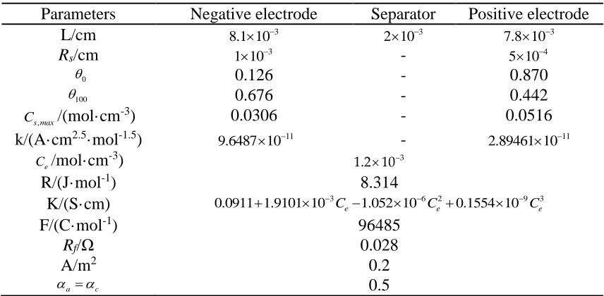
shows most of the model parameters of the 3.5 Ah 18650-type NCM cells that we chose. The cell structure parameters are derived from reference [19], such as the thickness and particle radius. The other parameters are adopted from references [20-22]. Otherwise, seven model parameters (Ds,n, Ds,p, εe,n，

εe,p, εe,s, εs,n and εs,p) are identified by the GA with temperature and current changes considered because

these parameters usually change with cell type and are closely associated with battery characteristics.

Table 1. Parameters for the electrochemical model of the LIBs

Parameters Negative electrode Separator Positive electrode

L/cm 3

8.1 10  2 10 3 7.8 10 3

Rs/cm 1 10 3 - 5 10 4

0

 _{0.126 - 0.870}

100

 _{0.676 - 0.442}

,

s max

C /(mol·cm-3) 0.0306 - 0.0516

k/(A·cm2.5·mol-1.5) 11

9.6487 10  - 11

2.89461 10 

e

C /mol·cm-3) _{1.2 10} 3

R/(J·mol-1) 8.314

K/(S·cm) _{0.0911 1.9101 10}  3 _{1.052 10} 6 2_{0.1554 10} 9 3

e e e

C C C

F/(C·mol-1) 96485

Rf/Ω 0.028

A/m2 _0.2

a c 0.5

2.2.2. Offline and online estimation

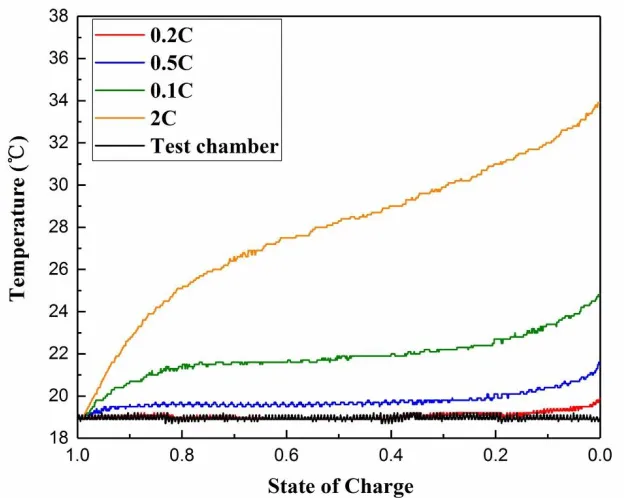
Figure 2. Temperature increases of cells at different current rates of 0.2, 0.5, 1 and 2C.

Table 2. Maximal temperature increase of cells under different current rates.

Current rate 0.2 0.5 1 2

Rise (C) 0.9 2.4 5.6 14.8

The GA is a global optimization probabilistic search algorithm modelled after natural evolution. During each evolution process, new individuals are generated by fitness-proportionate selection, and randomly selected crossover and mutation operations are applied to the genes of individuals [22]. The GA was applied to estimate the seven unknown parameters offline with the temperature and current considered; the corresponding flow chart is shown in Figure 3. Each GA individual includes 7 variables: Ds,n, Ds,p, εe,n，εe,p, εe,s, εs,n. and εs,p respectively. Table 3 shows the value ranges of the seven parameters.

The population size, number of genetic iterations, crossover probability Pc and mutation probability Pm

in the GA are set to 50, 100, 0.6 and 0.007, respectively. Furthermore, the following fitness function (28) of individuals is the sum of the squares of the output voltage errors between the simplified model and tested cells. The GA process is repeated at each temperature (10C, 20C, 30C and 40C) and each discharge current rate (0.2C, 0.5C, 1C and 2C) based on the collected experimental data, and the estimated results are listed in Table 4. From Figure 2, the temperature rise of 1C is below 3C when the SOC is as low as 0.2; therefore, the estimated results of discharge current rate (<1C) at different temperatures can be considered the true values of the corresponding temperature and prepared for lookup tables. However, the parameters associated with a discharge current rate of 2C should be estimated by the GA directly offline at different temperatures because of the drastic increase in temperature.





1

2

0







f U U (

Table 3. Value ranges of the parameters

,

s n

D Ds p, e n, e p, e s, s n, s p,

12 9

1 10  ~ 1 10  12 9

1 10  ~ 1 10  0~0.9 0~0.9 0~0.9 0~0.9 0~0.9

Figure 3. Theflow diagram of the GA for offline parameter identification.

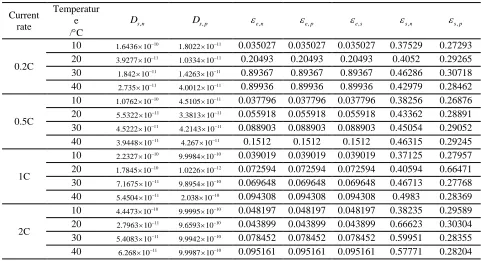
Table 4. Estimated model parameters related to discharge current rate and temperature.

Current rate

Temperatur e /C

,

s n

D Ds p, e n, e p, e s, s n, s p,

0.2C

10 _{1.6436 10} 10 _{1.8022 10} 11 _{0.035027 0.035027 0.035027 0.37529 0.27293}

20 11

3.9277 10  11

1.0334 10  0.20493 0.20493 0.20493 0.4052 0.29265

30 11

1.842 10  11

1.4263 10  0.89367 0.89367 0.89367 0.46286 0.30718

40 11

2.735 10  11

4.0012 10  0.89936 0.89936 0.89936 0.42979 0.28462

0.5C

10 10

1.0762 10  11

4.5105 10  0.037796 0.037796 0.037796 0.38256 0.26876

20 11

5.5322 10  11

3.3813 10  0.055918 0.055918 0.055918 0.43362 0.28891

30 11

4.5222 10  11

4.2143 10  0.088903 0.088903 0.088903 0.45054 0.29052

40 11

3.9448 10  11

4.267 10  0.1512 0.1512 0.1512 0.46315 0.29245

1C

10 10

2.2327 10  10

9.9984 10  0.039019 0.039019 0.039019 0.37125 0.27957

20 10

1.7845 10  12

1.0226 10  0.072594 0.072594 0.072594 0.40594 0.66471

30 _{7.1675 10} 11 _{9.8954 10} 10 _{0.069648 0.069648 0.069648 0.46713 0.27768}

40 11

5.4504 10  10

2.038 10  0.094308 0.094308 0.094308 0.4983 0.28369

2C

10 10

4.4473 10  10

9.9995 10  0.048197 0.048197 0.048197 0.38235 0.29589

20 _{2.7963 10} 11 _{9.6593 10} 10 _{0.043899 0.043899 0.043899 0.66623 0.30304}

30 11

5.4083 10  10

9.9942 10  0.078452 0.078452 0.078452 0.59951 0.28355

40 11

6.268 10  10

A 2-D lookup table based on the results estimated by the GA is utilized to describe the relationship between each parameter and the corresponding temperature/ discharge current rate (<1C) to realize real-time estimation because of the approach’s accuracy and celerity [23]. Each parameter of the model is a function of temperature T and discharge current rate C.





s s

D D T C





s s

D D T C





, , ,

_{e n}_{e n} T C





, , ,

e p e p T C





, , ,

e s e s T C





, , ,

s n s n T C





, , ,

s p s p T C

Each parameter is described by a 2-D lookup table (3 current breakpoints *4 temperature breakpoints) with discharge current rate and temperature as inputs, and the model parameter is the output. Internally, each parameter is evaluated by a linear interpolation method according to two inputs. The fidelity of the model can be improved by increasing the number of points related to discharge current rate and temperature, but introducing more breakpoints can also create two problems. First, introducing more points can increase the computational cost. Second, the benefit of introducing more points is diminishing, and an excessive number of breakpoints may generate numerous parameter values that are not consistent with the optimal solutions [24].

2.3. Sensitivity analysis of model parameters

Figure 4a-c shows the sensitivity analysis curves of εe,n, εe,p and εe,s separately, and their input

parameters are all varied with a fixed step size of 0.2. Even when the input parameter is sharply decreased to 0.04, the output curves are all anastomotic, which indicates that the three parameters are insensitive. The sensitivity analysis curves of Ds,n and Ds,p are shown in Figure 4d and e. The input values are set to

1.0e-11, 1.0e-10 and 1.0e-9 separately because of the broad value range relative to the order of magnitude. Figure 4f-g shows the sensitivity analysis curves of εs,n and εs,p. Their fixed step sizes are 0.1

and 0.05, respectively. As shown in Figure 4d-g, the output curves vary greatly, especially at the end of discharge, which demonstrates that the four parameters are sensitive parameters and that slight changes in their values can greatly influence the model’s fidelity. Therefore, εe,s is selected from three insensitive

parameters and assigned an optimal value of 0.30446, which is identified by GA at 25C.

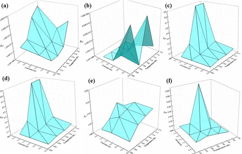
Figure 5. Fitting surfaces of the model parameters (a)Ds n, , (b)Ds p, , (c)e n, , (d) e p, , (e) s n, , and (f) s p, .

The relationships between the other model parameters, temperature and current are illustrated in Figure 5. In the negative electrode, Ds,n (Figure 5a) and εs,n (Figure 5e) both increase with increasing

temperature, but only Ds,n increases appreciably with increasing current. In the positive electrode, the

dependence of Ds,p (Figure 5b) and εs,p (Figure 5f) on temperature and current is distinct when the current

increases, showing an irregular shape with temperature. In the electrolyte phase, εe,n (Figure 5c) and εe,p

3. RESULTS AND DISCUSSION

3.1. Experimental verification

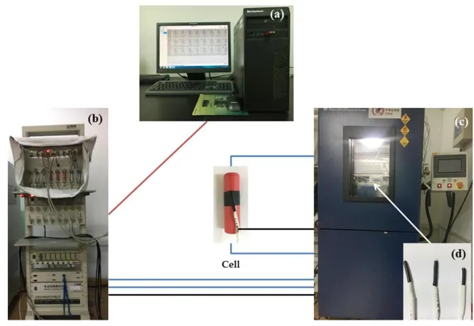
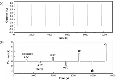
In this paper, 3.5 Ah NCM 18650-type cells are chosen to validate the simplified model and the proposed estimation method. The experiments include constant current discharge tests and two self-designed pulse current tests. A host computer for profile setting and date storage, a battery testing system (Shenzhen Neware Technology CO., LTD), a programmable fast thermal test chamber (MSK-TE906, Shengzhen Kejing Star Technology CO., LTD) and temperature sensors attached to the cells are shown in Figure 6. The cells are charged to 4.2 V by the standard constant-current constant-voltage (CCCV) scheme according to the manufacturer’s guidelines and discharged to 2.5 V at different current rates (0.2C, 0.5C, 1C and 2C) and temperatures (10C, 20C, 30C and 40C). The self-designed pulse current tests include two sections, and the current profiles are shown in Figure 7a and b, respectively. One is the 1C pulse discharge test, which is implemented over the range of 20%-90% SOC in steps of 10%. To validate the adaptation of the proposed method to different charge/discharge current rates, the other is a 4-step pulsed-current test applied with a current rate of 0.2C, 0.5C, 1C and 2C. For the two pulse discharges, the temperature increase is minute and ignored because the pulse time is too short relative to the rest time. In the figures, a positive current indicates discharge, and a negative current indicates charge.

Figure 7. Current profiles of (a) 1C pulse discharge and (b) 4-step pulsed-current tests.

3.2. Algorithm validation

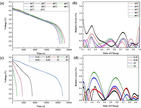
To verify the accuracy of the parameter identification algorithm and analyse the simplified model stability to various temperature and current effects, a comparison of the experimental and simulated terminal voltages under different temperatures and discharge rates is shown in Figure 8. Figure 8a and b describes the battery terminal voltage curves at different temperatures with a current of 0.2C and the corresponding relative error between experiment and simulation separately. The experimental and simulated curves almost overlap, and the voltage relative errors are essentially within 0.5%. The error at 25C is slightly larger than the errors at other temperatures because the model parameters at 10, 20, 30 and 40C are identified by the GA as breakpoints in 2-D lookup tables, but the parameters at 25C are estimated by linear interpolation method through 2-D lookup tables. Clearly, the error is also approximately 0.5%, except at the end of discharge at 25 °C; fortunately, however, the vehicle batteries mainly operate in the middle of the SOC, which indicates that the proposed method has high fidelity and strong robustness to temperature change.

Figure 8. Comparison of experimental data and simulation results under the effects of different temperatures at 10, 20, 30 and 40C (0.2C) (a). Relative error of temperature effect at different temperature (b) and discharge current rates 0.2, 0.5, 1 and 2C (20C) (c). Relative error of current effect (d). (  exp sim

exp

U U

Relative Error

U , the solid line is the experimental curve and the dashed line is the simulated curve).

3.3. Model validation

SOC), generally because the battery exhibits strong nonlinear characteristics at extreme SOC universally. There is good agreement between the simulated and actual charge/discharge voltages for 4 different current rates (Figure 9b), which demonstrates the excellent flexibility of the proposed model with changes in charge/discharge current rates.

Table 5. Cell voltage absolute error and simulation runtime of the three load profiles.

Load profile (20C)

Average error voltage

(mV)

Maximal error voltage

(mV)

Average relative error

(%)

Runtime (s)

1C discharge 11 56 0.2 0.803

1C pulse discharge

32 60 0.8 1.0

4-step pulse test 9 64 0.2 0.717

The voltage errors and simulation runtimes of the three load profiles are indicated in Table 5. The maximum voltage absolute errors for the 1C discharge, 1C pulse discharge and 4-step pulse tests are all below 65 mV, and the average relative errors are 0.2%, 0.8% and 0.2%, respectively. The simulation runtimes of the three load profiles are 0.803, 1.0 and 0.717 s, respectively, which are remarkably short and verify the simplicity and practicality of the simplified model.

Table 6. Comparison with reported works at 1C discharge

References Model used Algorithm Voltage error Temperature/current

dependence The paper Electrochemical

model

Genetic algorithm 0~0.056 V/0~0.7%/ 0.2%(average)

Yes

16 Electrochemical-thermal coupling

model

Least-squares fit 0~0.07 V Temperature

26 Multi-physics model Genetic algorithm 0~0.0763 V Temperature

27 Electrothermal model

Least-squares nonlinear algorithm

0~1% Temperature

28 SPM - 0~1% Temperature

29 Simplified P2D - 0~0.4% No

30 Electrochemical model

- 0.2076% (average) No

31 Electrochemical model

Genetic algorithm 0~0.1 V No

32 Electrochemical model

Bacterial foraging optimization

algorithm

0~0.08 V No

33 Electrochemical model

Least squares 0~1% current

34 ECM Least-squares curve

fitting

0~1.23%/ 0.29% (average)

Yes

35 ECM with improved P2-D model

Recursive least squares

0~0.06 V No

36 Splice-ECM Curve fitting 0~2% No

37 ECM Extend Kalman filter 0.12% (average) No

In short, the flexible simplified model established by the proposed method is verified to be effective in reducing computational cost and maintaining high fidelity. The results are mainly attributed to two reasons: one is that the simplified model is greatly reduced with partial internal information loss but captures the dynamic characteristics very well, and the other is utilizing the proposed parameter identification method to relieve the influence of temperature and current on the model’s performance and maintain the strong stability of the model.

4. CONCLUSION

In this paper, a simplified electrode-average model reduced using polynomial approximation and a three-variable method is proposed, which not only captures the dynamic behaviour of a battery but also simplifies the physics-based equations of the solid and electrolyte phases to reduce model complexity. A practical method is developed for identifying the model parameters employing the genetic algorithm from observed experimental data to create 2-D lookup tables with temperature and current as independent variables for online estimation. The model parameters are estimated directly for large discharge current rate, under which the temperature rises sharply during discharge. To validate the simplified model and the proposed estimation method, 3.5 Ah NCM 18650-type cells are selected. The results suggest that the simple method possesses low complexity, sufficient accuracy and excellent adaptability to changes in temperature and current rate. The simplified model combined with the proposed parameter identification method updates the parameters with a voltage error of 0~0.056 V, a relative voltage error of 0~0.7% and an average relative error of 0.2%.

ACKNOWLEDGMENTS

The research is supported by Special Funds for the Transformation of Scientific and Technological Achievements in Jiangsu Province (BA2016162), the National Science and Technology Foundation of China (2015BAG07B00), NSFC (21501071), the Six Talents Peak Project of Jiangsu Province (2016-XNYQC-003, 2015-XNYQC-008), and the Foundation for Advanced Talents of Jiangsu University (13JDG071, 12JDG054).

NOMENCLATURE

j Reaction flux at the solid particle surface, [mol cm-1 s-1]

s

C _{Concentration of Li}+ _{ions in an electrode particle, [mol cm}-3_]

s

D _{Diffusion coefficient of lithium in an electrode particle, [cm}2 _s]

s

a _{Specific surface area of electrode, [cm}-1_]

F Faraday’s constant, [C mol-1_]

i

R _{Radius of solid particles, [cm]}

eff Effective electronic conductivity of solid particles, [S cm-1]

s Solid-phase potential, [V]

A Electrode plate area, [cm2]

L Total cathode-separator-anode thickness, [cm]

eff

K Effective ionic conductivity of the electrolyte phase, [S cm-1] eff

D

K Effective ionic diffusional conductivity of the electrolyte phase, [S cm-1]

e Volume fraction of the electrolyte phase

e

C _{Concentration of Li}+ _{ions in the electrolyte phase, [mol cm}-3_]

0



t _{Lithium ion transference number in the electrolyte} T Absolute temperature, [K]

R Universal gas constant

0

i _{Exchange current density, [A cm}-2_]

k Intercalation/deintercalation reaction-rate constant of electrode, [A·cm2.5·mol-1.5 ]  _{Overpotential, [V]}

,

s max

C _{Maximum concentration of Li}+ _{ions in the particle of electrode, [mol cm}-3_]

,

s surf

C _{Surface concentration of Li}+ _{ions in the particle of electrode, [mol cm}-3_]

f

R _{Film resistance, [Ω]} p Positive electrode n Negative electrode

a, c Anodic and cathodic transfer coefficients

References

1. L. Lu, X. Han, J. Li, J. Hua and M. Ouyang, J. Power Sources, 226 (2013) 272.

3. V. Ramadesigan, P. W. C. Northrop, S. De, S. Santhanagopalan, R.D. Braatz and V. R. Subramanian, Multi-scale Modeling and Simulation of Lithium-Ion Batteries from Systems Engineering Perspective, 220th ECS Meeting, Boston, America, 2011, Abstract 747.

4. K. E. Thomas, J. Newman and R. M. Darling, Advances in Lithium-Ion Batteries, Springer, (2002) Boston, USA.

5. J. Newman and K. E. Thomasalyea, Electrochemical Systems, John Wiley & Sons, (2004) Canada. 6. M. Doyle, T. F. Fuller and J. Newman, J. Electrochem. Soc., 140 (1993) 1526.

7. S. De, B. Suthar, D. Rife, G. Sikha and V. R. Subramanian, J. Electrochem. Soc., 160 (2013), A1675. 8. D. D. Domenico, A. Stefanopoulou and G. Fiengo, J. Dyn. Syst. Meas. Control, 132 (2010) 768. 9. L. Cai and R. E. White, J. Electrochem. Soc., 156 (2009) A154.

10. C. Yuan, B. Wang, H. Zhang, L. Chen and H. Li, Int. J. Electrochem. Sci., 13 (2018) 1131. 11. M. Chen and G. A. Rincon-Mora, IEEE T. Energy Conver., 21 (2006) 504.

12. A. Jossen, J. Power Sources, 154 (2006) 530.

13. S. Yuan, L. Jiang, C. Yin, H. Wu and X. Zhang, J. Power Sources, 352 (2017) 245. 14. W. Shen, H. Li, Energies, 10 (2017) 432.

15. J. C. Forman, S. J. Moura, J. L. Stein and H. K. Fathy, J. Power Sources, 210 (2012) 263. 16. J. Li, L. Wang, C. Lyu, H. Wang and X. Liu, J. Power Sources, 307 (2016) 220.

17. T. S. Dao, C. P. Vyasarayani and J. Mcphee, J. Power Sources, 198 (2012) 329.

18. V. R. Subbramanian, V. D. Diwakar and D. Tapriyal, J. Electrochem. Soc., 150 (2005) A2002. 19. Y. Ji, Y. Zhang and C. Wang, J. Electrochem. Soc., 160 (2013) A636.

20. X. Han, M. Ouyang, L. Lu and J. Li, J. Power Sources, 278 (2015) 814.

21. S. K. Rahimian, S. Rayman and R. E. White, J. Power Sources, 224 (2013) 180-194.

22. T. R. Ashwin, A. Mcgordon, W. D. Widanage and P. A. Jennings, J. Power Sources, 341 (2017) 387.

23. C. Wang, T. He, X. Liu, S. Zhong, W. Chen and Y. Feng, Magn. Reson. Med., 73 (2015) 865. 24. R. A. Jackey, G. L. Plett and M. J. Klein, SAE World Congress & Exhibition, Detroit, USA, 2009,

SAE paper 2009-01-1381.

25. T. Turányi and A. S. Tomlin, Analysis of Kinetic Reaction Mechanisms, Springer, (2014) Berlin Heidelberg, Germany.

26. L. Zhang, L. Wang, G. Hinds, C. Lyu, J. Zheng and J, Li, J. Power Sources, 270 (2014) 367. 27. S. N. Motapon, A. Lupien-Bedard, L. A. Dessaint, H. Fortin-Balanchette and K. Al-Haddad, IEEE

T. Ind. Electron., 64 (2017) 998.

28. T. R. Tanim, C. D. Rahn and C. Y. Wang, J. Dyn. Syst. Meas. Control, 137 (2014) 011005. 29. P. Kemper, S. E. Li and D. Kum, J. Power Sources, 286 (2015) 510.

30. N. Lotfi, R. G. Landers, J. Li and J. Park, IEEE T. Contr. Syst. T., 25 (2017) 1217. 31. X. Xu, W. Wang and L. Chen, J. Electrochem. Soc., 163 (2016) A1429.

32. Y. Ma, J. Ru, M. Yin, H. Chen and W. Zheng, J. Appl. Electrochem., 46 (2016) 1119. 33. G. K. Prasad and C. D. Rahn, J. Power Sources, 232 (2013) 79.

34. Y. Zhang, Y. Shang. N. Cui and C. Zhang, Energies, 11 (2018) 19. 35. X. Zhang, J. Lu, S. Yuan and X. Zhou, J. Power Sources, 345 (2017) 21.

36. S. Wang, C. Fernandez, X. Liu, J. Su and Y. Xie, Meas. Control-Uk, 51 (2018) 125. 37. X. Zhang, Y. Wang, D. Yang and Z. Chen, Energy, 115 (2016) 219.