STRUCTURED ROBUST STABILITY AND BOUNDEDNESS OF
NONLINEAR HYBRID DELAY SYSTEMS\ast
WEIYIN FEI\dagger , LIANGJIAN HU\ddagger , XUERONG MAO\S , AND MINGXUAN SHEN\P Abstract. Taking different structures in different modes into account, the paper has developed a new theory on the structured robust stability and boundedness for nonlinear hybrid stochastic differential delay equations (SDDEs) without the linear growth condition. A new Lyapunov function is designed in order to deal with the effects of different structures as well as those of different parameters within the same modes. Moreover, a lot of effort is put into showing the almost sure asymptotic stability in the absence of the linear growth condition.
Key words. hybrid SDDEs, robust stability, robust boundedness, Brownian motion, Markov chain
AMS subject classifications. 60H10, 60J10, 93E15
DOI. 10.1137/17M1146981
1. Introduction. Systems in many branches of science and industry not only de-pend on the present state and the past ones but may also experience abrupt changes in their structures and parameters. Hybrid stochastic differential delay equations (SDDEs; also known as SDDEs with Markovian switching) have been widely used to model these systems (see, e.g., the books [23, 24] and the references therein). One of the important issues in the study of hybrid SDDEs is the asymptotic analysis of stability and boundedness (see, e.g., [3, 5, 13, 19]). In asymptotic analysis, robust stability and boundedness have been two of most popular topics. For example, Ack-ermann [1] gave a nice motivation of robust stability. Hinrichsen and Pritchard [7, 8] presented an excellent discussion of the stability radii of linear systems with struc-tured perturbations. Su [26] and Tseng, Fong, and Su [27] discussed robust stability for linear delay equations. In the aspect of robustness of stochastic stability, Hauss-mann [6] studied robust stability for a linear system and Ichikawa [11] for a semilinear system. Mao, Koroleva, and Rodkina [21] discussed the robust stability of uncertain linear or semilinear stochastic delay systems. Mao [20] investigated the stability of the stochastic delay interval system with Markovian switching. For more information on the stability and boundedness of hybrid SDDEs, please see, e.g., [12, 22, 23, 25]. However, all of the papers, up to 2013, in this area only considered these robust
\ast Received by the editors September 11, 2017; accepted for publication (in revised form) May 21,
2018; published electronically July 17, 2018.
http://www.siam.org/journals/sicon/56-4/M114698.html
Funding: The work of the authors was supported by the Royal Society (WM160014, Royal Society Wolfson Research Merit Award), the Royal Society and the Newton Fund (NA160317, Royal Society-Newton Advanced Fellowship), the EPSRC (EP/K503174/1), the Natural Science Foundation of China (11471071, 71571001), and the Ministry of Education (MOE) of China (MS2014DHDX020).
\dagger School of Mathematics and Physics, Anhui Polytechnic University, Wuhu, Anhui 241000, China
\ddagger Corresponding author. Department of Applied Mathematics, Donghua University, Shanghai
201620, China ([email protected]).
\S Department of Mathematics and Statistics, University of Strathclyde, Glasgow G1 1XH, UK ([email protected]).
\P School of Mathematics and Physics, Anhui Polytechnic University, Wuhu, Anhui 241000, China, and School of Science, Nanjing University of Science and Technology, Nanjing, Jiangsu 210094, China ([email protected]).
2662
problems where the underlying systems were either linear or nonlinear with the linear growth condition (i.e., the coefficients are bounded by a linear function).
Hu, Mao, and Zhang [9] were the first to investigate robust stability and
bound-edness for nonlinear hybrid SDDEswithout the linear growth condition (i.e., the
co-efficients are not bounded by a linear function, and we will refer to these coco-efficients as highly nonlinear functions). The significant contribution of [9] lies in that it shows that a given stable hybrid SDDE can tolerate not only the linear-type perturbation but also the highly nonlinear perturbation without loss of the stability, while the pa-pers up to 2013 could only cope with the linear-type perturbation. In other words, Hu, Mao, and Zhang [9] opened a new chapter in the study of robust stability for highly nonlinear hybrid SDDEs. However, the progress in this direction is due some-what to the difficulty of high nonlinearity, and [9] is the only paper so far, to the best of our knowledge. The aim of this paper is to make some further progress in this area. Let us explain our key motivation briefly here, though further details will be given in section 3. As we know, hybrid SDDEs have been used to model practical systems that may experience abrupt changes in their structures and parameters (see, e.g., [3, 5, 13, 23]). The theory in [9] is good at dealing with hybrid SDDEs that may experience abrupt changes in their parameters. To explain this, assume that a population system operates in two modes, dry and rain, and it switches from one mode to the other according to a two-state Markov chain with state 1 for dry and state 2 for rain. In the dry mode, the system is described by a stochastic delay Lotka--Volterra equationdx(t) =x(t)([a1 - b1x2(t)]dt+\sigma 1x(t - \tau )dB(t)), while in the rain mode by another equationdx(t) =x(t)([a2 - b2x2(t)]dt+\sigma 2x(t - \tau )dB(t)), where\tau >0 stands
for the time delay, a1, b1, a2, b2 are all positive numbers, B(t) is a scalar Brownian
motion, and\sigma 1, \sigma 2 represent the intensities of the nonlinear stochastic perturbation.
In other words, the population system is described by the hybrid SDDE dx(t) =
x(t)([ar(t) - br(t)x2(t)]dt+\sigma r(t)x(t - \tau )dB(t)). This can be regarded as a stochastically
perturbed system of the hybrid delay systemdx(t)/dt=x(t)[ar(t) - br(t)x2(t)] with the
highly nonlinear stochastic perturbation\sigma r(t)x(t)x(t - \tau )dB(t). Given the asymptotic
boundedness of the delay system dx(t)/dt = x(t)[ar(t) - br(t)x2(t)], the theory in
[9] shows the upper bounds on \sigma 1 and \sigma 2 for the SDDE to remain asymptotically
bounded. We observe that in this example, when the system switches from one mode
to the other, only the system parameters change, but the structure of the system
remains the same type of Lotka--Volterra. On the other hand, many practical systems may experience abrupt changes in their structures. For example, a population system may change from a delay geometric Brownian motion dx(t) = - 2x(t)dt+\sigma 1x(t - \tau )dB(t) in the dry mode to a delay Lotka-Volterra equationdx(t) =x(t)[1 - 2x2(t)]dt+
\sigma 2x2(t - \tau )dB(t) in the rain mode (see, e.g., [2]); a financial system may switch from a geometric Brownian motiondx(t) =a1x(t)dt+\sigma 1x(t)dB(t) to a constant elasticity of volatility (CEV) processdx(t) =a2(\mu - x(t))dt+\sigma 2x1.5(t)dB(t) (see, e.g., [15]). Is
the theory in [9] applicable to such hybrid SDDEs? We will show a negative answer in section 3. This motivates us to develop a new theory on the robust stability and boundedness for highly nonlinear hybrid SDDEs which may experience abrupt changes in their structures.
To make our theory more general, we consider the case where the space of modes,
S, of a given hybrid system can be divided into two proper subspaces,S1andS2, such
that the system is described by the same type of SDDEs for modes in S1 (though
different parameters for different modes of course) but by a different type of SDDEs
for modes in S2. For example, for the population system in the second half of the
last paragraph, we haveS =\{ dry, rain\} , S1 =\{ dry\} , S2 =\{ rain\} , and the system
is described by a delay geometric Brownian motion for a mode in S1 but by a delay
Lotka--Volterra equation for a mode in S2. Of course, in our setting, both S1 and
S2 could contain 2 or more modes (see Example 6.2). We should point out that it
is possible to develop our theory to cope with the even more general case where S
can be divided into more than two subspaces, and the structures of the underlying hybrid SDDE are significantly different among these subspaces. However, to avoid our notation becoming too complicated, we will only concentrate on the case of two subspaces in this paper.
The key contributions of our paper are highlighted below:
\bullet This is the first paper that takes the different structures in different modes into
account to develop a new theory on structured robust stability and bound-edness for highly nonlinear hybrid SDDEs.
\bullet The new theory established in this paper is applicable to hybrid SDDEs which
may experience abrupt changes in both structures and parameters.
\bullet The stabilities discussed in this paper include not only the pth moment and
almost sure exponential stability but also the pth moment and almost sure
asymptotic stability as well as H\infty stability. (For the definitions of these
stabilities we refer the reader to [9, 23].)
\bullet A significant amount of new mathematics has been developed to deal with
the difficulties due to the structured difference and those without the linear growth condition. For example, a new Lyapunov function will be designed
in order to deal with the effects of different structures forS1-modes and S2
-modes as well as the effects of different parameters withinS1 andS2. A lot
of effort has also been put into showing the almost sure asymptotic stability without the linear growth condition.
To develop our new theory, we will introduce some necessary notation in section 2. We will show in section 3 that the theory in [9] is not applicable to hybrid SDDEs which may experience abrupt changes in structures, and this motivates us to establish a new theory in this paper. Our main results on robust boundedness and stability will be discussed in sections 4 and 5. We will present some case studies and examples in section 6 to illustrate our theory. We will finally conclude our paper in section 7.
2. Notation. Throughout this paper, unless otherwise specified, we use the fol-lowing notation. Let (\Omega ,\scrF ,\{ \scrF t\} t\geq 0, P) be a complete probability space with a
fil-tration \{ \scrF t\} t\geq 0 satisfying the usual conditions (i.e., it is increasing and right
con-tinuous while \scrF 0 contains all P-null sets). Let B(t) = (B1(t), . . . , Bm(t))T be an
m-dimensional Brownian motion defined on the probability space. Letr(t), t\geq 0, be
a right-continuous-left-limit Markov chain on the probability space taking values in a finite state spaceS=\{ 1,2, . . . , N\} with generator \Gamma = (\gamma ij)N\times N given by
P\{ r(t+ \Delta ) =j| r(t) =i\} = \biggl\{
\gamma ij\Delta +o(\Delta ) ifi\not =j, 1 +\gamma ij\Delta +o(\Delta ) ifi=j,
where \Delta > 0. Here \gamma ij \geq 0 is the transition rate from i to j if i \not = j while \gamma ii =
- \sum
j\not =i\gamma ij. We assume that the Markov chain r(\cdot ) is independent of the Brownian motionB(\cdot ). We also denote by| x| the Euclidean norm forx\in Rn. IfAis a vector or
matrix, its transpose is denoted byAT. IfAis a matrix, its trace norm is denoted by
| A| =\sqrt{} trace(ATA). LetR+= [0,\infty ) and\tau >0. Denote byC([ - \tau ,0];Rn) the family
of continuous functions \xi from [ - \tau ,0] to Rn with the norm\| \xi \| = sup
- \tau \leq \theta \leq 0| \xi (\theta )| .
If bothaandbare real numbers, thena\vee b= max\{ a, b\} anda\wedge b= min\{ a, b\} . IfG
is a set, its indicator function is denoted by IG. That is,IG(x) = 1 if x\in Gand 0
otherwise.
We also need some notation on M-matrices. For a vector or matrixA, byA >0
we mean all elements ofAare positive. AZ-matrix is a square matrixA= (aij)N\times N which has nonpositive off-diagonal entries (namely aij \leq 0 for alli \not = j). The
fol-lowing lemma provides us with two useful criteria to verify if a given Z-matrix is a
nonsingular M-matrix (see, e.g., [4, 9, 23]).
Lemma 2.1. LetA= (aij)N\times N be aZ-matrix. ThenAis a nonsingularM-matrix
if and only if one of the following statements holds: (1) A - 1 exists and its elements are all nonnegative. (2) There existsx >0 in RN such thatAx >0.
By this lemma, we see, for example, that for any positive numbers\varepsilon i (i\in S),
A:= diag(\varepsilon 1, . . . , \varepsilon N) - \Gamma is a nonsingular M-matrix asA(1, . . . ,1)T = (\varepsilon 1, . . . , \varepsilon
N)>0. This useful technique
will be used quite often when we discuss some special cases in section 6 below.
3. Motivation. To motivate our new study in this paper, let us recall a key
result on robust stability from [9]. Consider an n-dimensional hybrid differential
equation
(3.1) dx(t)
dt =F(x(t), t, r(t))
ont\geq 0 and assume that this hybrid system is subject to a stochastic delay
pertur-bation and the perturbed system is described by a hybrid SDDE
(3.2) dx(t) =F(x(t), t, r(t))dt+G(x(t - \tau ), t, r(t))dB(t).
Here r(t), B(t), and\tau have been defined in section 2; both F :Rn\times R+\times S \rightarrow Rn
andG:Rn\times R+\times S\rightarrow Rn\times mare Borel measurable and locally Lipschitz continuous
in the first variable. In [9], the following assumption was imposed.
Assumption 3.1. Letq > p\geq 2 and assume that for eachi\in S, there are a real number \=\beta i2 and a nonnegative number \=\beta i4 such that
(3.3) xTF(x, t, i)\leq \beta \=i2| x| 2 - \beta \=i4| x| q - p+2
for all (x, t)\in Rn\times R
+, and
(3.4) \scrA \=:= - diag(p\beta 12, . . . , p\= \beta \=N2) - \Gamma
is a nonsingular M-matrix.
It is shown in [9] that this assumption along with the local Lipschtiz condition
guarantees the pth moment exponential stability of the given equation (3.1). The
study of the robust stability is to investigate how much of the stochastic delay pertur-bationG(x(t - \tau ), t, r(t))dB(t) the given stable equation (3.1) can tolerate so that its perturbed system (3.2) remains stable. To measure the stochastic delay perturbation more precisely, the following assumption was then imposed in [9].
Assumption 3.2. Let q > p \geq 2 be the same as in Assumption 3.1 and assume that for eachi\in S, there are nonnegative numbers \=\beta i3and \=\beta i5 such that
(3.5) | G(y, t, i)| 2\leq \beta \=
i3| y| 2+ \=\beta i5| y| q - p+2
for all (y, t)\in Rn\times R+.
The study of the robust stability is then to give the bounds on the parameters \=
\beta i3 and \=\beta i5 in order for the perturbed system (3.2) to remain stable. The following
theorem describes this situation.
Theorem 3.3 (see [9, Theorem 3.4]). Let Assumptions 3.1 and 3.2 hold. As-sume thatF(0, t, i) =G(0, t, i) = 0for allt\geq 0andi\in S. Define
(3.6) (\=\theta 1, . . . ,\theta \=N)T := \=\scrA - 1(1, . . . ,1)T
(so all \theta \=i's are positive). If
(3.7) \beta \=i3<
2
p(p - 1)\=\theta i
and \beta \=i5<
2 minj\in S\theta \=j\beta \=j4
(p - 1)\=\theta i
for alli\in S, then the perturbed system (3.2)is exponentially stable in thepth moment.
The significant contribution of this theorem lies in that it shows not only how much of the linear perturbation (controlled by \sqrt{} \beta \=i3| y| ) but also how much of the
nonlinear perturbation (controlled by \sqrt{} \beta \=i5| y| q - p+2) the given stable equation (3.1)
can tolerate without loss of the stability, while the existing papers up to 2013 could only cope with the linear perturbation as pointed out in section 1.
However, we shall now point out its limitation. Recall the population system stated in section 1: It operates in two modes: dry and rain. Assume that the switching between the two modes is modeled by a Markov chainr(t) on the state spaceS=\{ 1,2\}
(1 for dry and 2 for rain) with the generator
(3.8) \Gamma =
\biggl(
- 1 1
6 - 6 \biggr)
.
The system is modeled by the hybrid SDDE
(3.9) dx(t) =F(x(t), r(t))dt+G(x(t - \tau ), r(t))dB(t),
whereB(t) is a scalar Brownian motion and
F(x,1) = - 2x, F(x,2) =x - 2x3, G(y,1) =\sigma 1y, G(y,2) =\sigma 2y2
for x, y \in R, in which both \sigma 1 and \sigma 2 are positive constants. That is, the system satisfies a delay geometric Brownian motiondx(t) = - 2x(t)dt+\sigma 1x(t - \tau )dB(t) in the dry mode but a delay Lotka--Volterra equationdx(t) =x(t)[1 - 2x2(t)]dt+\sigma 2x2(t - \tau )dB(t) in the rain mode. In other words, the system experiences abrupt changes in
their structures when it switches from one mode to the other. If both \sigma 1 = 0 and
\sigma 2= 0, (3.9) becomes
(3.10) dx(t)
dt =F(x(t), r(t)).
In other words, (3.9) is a stochastically perturbed system of (3.10). Noting that
xF(x,1) = - 2x2 and xF(x,2) =x2 - 2x4,
we see that condition (3.3) holds withp= 2,q= 4, and
\=
\beta 12= - 2, \beta 14\= = 0, \beta 22\= = 1, \beta 24\= = - 2.
Thus, by (3.4),
\=
\scrA =
\biggl(
5 - 1
- 6 4
\biggr)
with \=\scrA - 1= 1
14 \biggl(
4 1
6 5
\biggr)
.
So \=\scrA is a nonsingular M-matrix. In other words, Assumption 3.1 is satisfied. This
implies that (3.10) is exponentially stable in mean square. We expect that (3.10) can tolerate a liner perturbation\sigma 1x(t - \tau )dB(t) in mode 1 and a nonlinear perturbation
\sigma 2x2(t - \tau )dB(t) in mode 2 given its linear and nonlinear structure in modes 1 and
2, respectively. The aim here is to obtain upper bounds on \sigma 1 and \sigma 2 so that the
perturbed system (3.9) remains stable. Noting that
| G(y,1)| 2=\sigma 2
1y
2 and | G(y,2)| 2=\sigma 2
2y
4,
we see that Assumption 3.2 is satisfied withp= 2,q= 4, and
\=
\beta 13=\sigma 12, \beta \=15= 0, \beta \=23= 0, \beta \=25=\sigma 22.
To apply Theorem 3.3, we get \=\theta 1 = 5/14 and \=\theta 2= 11/14 by (3.6). Hence, condition (3.7) becomes
(3.11) \sigma 21<14/5 and \sigma 22<0.
Unfortunately, we never have\sigma 2
2 <0 so Theorem 3.3 is not applicable to the hybrid
SDDE (3.9). This indicates that the theory in [9] may not be applicable to the hybrid SDDEs that may experience abrupt changes in their structures.
4. Robust boundedness. Consider ann-dimensional hybrid SDDE
(4.1) dx(t) =f(x(t), x(t - \tau ), t, r(t))dt+g(x(t), x(t - \tau ), t, r(t))dB(t)
on t \geq 0 with initial data \{ x(\theta ) : - \tau \leq \theta \leq 0\} = \xi \in C([ - \tau ,0];Rn), where the
coefficientsf : Rn\times Rn\times R+\times S \rightarrow Rn and g : Rn\times Rn\times R+\times S \rightarrow Rn\times m are Borel measurable. As a standing hypothesis, we assume the coefficients are locally Lipschitz continuous (see, e.g., [16, 17]).
Assumption 4.1. For each integerh\geq 1 there is a positive constantKhsuch that
| f(x, y, t, i) - f(\=x,y, t, i\= )| 2\vee | g(x, y, t, i) - g(\=x,y, t, i\= )| 2
\leq Kh(| x - x\=| 2+| y - y\=| 2)
for thosex, y,x,\= y\=\in Rn with| x| \vee | y| \vee | x\=| \vee | y\=| \leq hand all (t, i)\in R+\times S.
It is very easy to verify this local Lipschitz assumption. For example, the
as-sumption is satisfied if f and g are continuously differentiable in x and y or they
are differentiable in xandy with locally bounded derivatives. It is known that this
classical assumption covers many hybrid SDDEs in the real world (see, e.g., the books [23, 24] and the references therein). Of course, this assumption is not enough to guar-antee the global solution (i.e., no explosion at a finite time). A standard additional condition for the existence and uniqueness of the global solution of the SDDE (4.1) would be the linear growth condition (see, e.g., [18, 23]). However, our aim here is to study the structured robust stability and boundedness of highly nonlinear SDDEs that do not satisfy the linear growth condition. We hence need to propose alternative assumptions.
Assumption 4.2. Assume that the state space S of the Markov chain is divided
into two proper subspacesS1and S2, and we may, without loss of any generality, let
S1 =\{ 1, . . . , N1\} and S2 =\{ N1+ 1, . . . , N\} , where 1\leq N1< N. Assume also that
there are two constants q > p\geq 2. Assume furthermore that for eachi\in S1, there
are constants\alpha i2\in Rand\alpha i1, \alpha i3\in R+ such that, for all (x, y, t)\in Rn\times Rn\times R+,
(4.2) xTf(x, y, t, i) +q - 1
2 | g(x, y, t, i)|
2\leq \alpha
i1+\alpha i2| x| 2+\alpha i3| y| 2;
while for each i \in S2, there are constants \alpha i2 \in R, \alpha i4 >0, and\alpha i1, \alpha i3, \alpha i5 \in R+
such that
xTf(x, y, t, i) +p - 1
2 | g(x, y, t, i)|
2
\leq \alpha i1+\alpha i2| x| 2+\alpha i3| y| 2 - \alpha i4| x| q - p+2+\alpha i5| y| q - p+2.
(4.3)
The reason why S is divided into two proper subspaces S1 and S2 is because
the structure of the underlying hybrid SDDE in S1-modes differs from that in S2
-modes, as explained in section 1. In terms of mathematics, conditions (4.2) and (4.3) describe the difference in structure. More understandably, condition (4.2) means that
the hybrid SDDE inS1-modes satisfies the classical Khasminskii-type condition (see,
e.g., [14, 23]) while condition (4.2) means that the hybrid SDDE inS2-modes satisfies
the generalized Khasminskii-type condition (see, e.g., [10]). In layman's terms, the
coefficients of the SDDE in S1-modes may grow linearly in the delay component
x(t - \tau ) while in S2-modes it may grow polynomially. It is easy to show whether a function grows linearly or polynomially, and hence it is not difficult to verify our Assumption 4.2, as demonstrated in our examples in section 6.
Noting that in Assumption 4.2, we only require\alpha i2\in R for alli\in S. According
to the Khasminskii-type theorems (see, e.g., [14, 10, 23]), the solution of the hybrid SDDE may grow exponentially. But our aim in this paper is to study the asymptotic boundedness and stability. We therefore need to impose some additional conditions on\alpha i2's.
Assumption 4.3. Under Assumption 4.2, assume furthermore that
(4.4) A:= - diag(p\alpha 12, . . . , p\alpha N2) - \Gamma
and
(4.5) D:= - diag(q\alpha 12, . . . , q\alpha N12) - (\gamma ij)i,j\in S1
are both nonsingular M-matrices.
This assumption means that some\alpha i2must be negative; otherwiseAandDcould
not be nonsingular M-matrices. Hence, the SDDE in modei with\alpha i2<0 should be
asymptotically bounded or stable. Of course, the SDDE in modeiwith\alpha i2\geq 0 could
still grow. However, conditions (4.4) and (4.5) mean that the switchings from those modes with \alpha i2 \geq 0 to those with \alpha i2 < 0 are sufficiently fast so that, overall, the
underlying hybrid SDDE is still asymptotically bounded or stable. We should also
point out that Assumption 4.3 can be verified easily. In fact, computeA - 1 andD - 1
easily using MATLAB or R and then check if their elements are all nonnegative. If so, by Lemma 2.1, they are nonsingular M-matrices.
When we design our Lyapunov function (see (4.15)), we will need two sets of numbers
(4.6) (\theta 1, . . . , \theta N)T =A - 1(1, . . . ,1)T
and
(4.7) (\eta 1, . . . , \eta N1)
T =D - 1(\beta , . . . , \beta )T,
where\beta is a free positive parameter. Under Assumption 4.3, we see, by Lemma 2.1,
that all\theta i (i\in S) and\eta i (i\in S1) are positive. We will see that\beta plays a key role in
balancing the effects of different structures forS1-modes andS2-modes. In particular,
if we choose \beta sufficiently small, then all \eta i will be small too. This means that we
can always make condition (4.9) in the following theorem possible by choosing \beta
sufficiently small. In particular, let us state a remark where we show a simple method
on how to determine\beta to guarantee condition (4.9).
Remark 4.4. Let \~d be the maximum of the row sums of D - 1 and \~\gamma = max
i\in S2 \cdot (\sum
j\in S1\gamma ij). Then \eta i \leq \beta
\~
d for all i \in S1 and \sum j\in S1\gamma ij\eta j \leq \beta
\~
d\~\gamma for all i \in S2.
Hence, if we choose
(4.8) \beta =mini\in S2p\theta i\alpha i4
1 + \~d\~\gamma ,
then condition (4.9) is guaranteed.
Let us now state our first result in this paper.
Theorem 4.5. Let Assumptions4.1,4.2, and 4.3hold. Choose\beta >0sufficiently small for
(4.9) \alpha i4\geq
\beta +\sum
j\in S1\gamma ij\eta j p\theta i
\forall i\in S2,
where\theta i and\eta i have been defined by (4.6)and (4.7). Assume also that
\alpha i3\leq
1
p\theta i
\forall i\in S,
(4.10)
\alpha i3< \beta \eta i(2q - p)
\forall i\in S1,
(4.11)
and
(4.12) \alpha i5<
\beta q \theta ip(2q - p)
\forall i\in S2.
Then for any initial data\xi \in C([ - \tau ,0];Rn), there is a unique global solutionx(t)to
the hybrid SDDE (4.1)ont\in [ - \tau ,\infty ). Moreover, the solution has the properties that
(4.13) lim sup
t\rightarrow \infty 1
t
\int t
0
E| x(s)| qds\leq K1
and
(4.14) lim sup
t\rightarrow \infty
E| x(t)| p\leq K2,
whereK1 andK2 are positive constants independent of the initial data\xi .
Before the proof, let us give some insight on the relevance of this theorem. We have explained that Assumptions 4.1, 4.2, and 4.3 cover many hybrid SDDEs in the
real world while they can be verified easily. Remark 4.4 shows at least one way of
determining \beta to make condition (4.9) hold. The right-hand-side terms of
inequali-ties (4.10)--(4.12) can then be computed straightaway, and these inequaliinequali-ties give the bounds on the nonlinear perturbation intensities \alpha i3 and\alpha i5 so that the underlying
hybrid SDDE is bounded inLp asymptotically as well as in the time-average of Lq.
Proof. The proof is very technical. To make it more understandable, we will divide it into several steps.
Step 1. In this step, we will define a Lyapunov functionV :Rn\times S\rightarrow R+ by
(4.15) V(x, i) =
\biggl\{
\theta i| x| p+\eta i| x| q ifi\in S1,
\theta i| x| p ifi\in S2
and show that it has some nice properties. First, it is easy to see that
(4.16) c1| x| p\leq V(x, i)\leq c2(| x| p+| x| q),
where
c1= min
i\in S\theta i, c2= \Bigl(
max i\in S \theta i
\Bigr)
\vee \Bigl( max
i\in S1 \eta i
\Bigr)
.
By the generalized It\^o formula (see, e.g., [23, Theorem 1.45, page 48]), we have that
(4.17) dV(x(t), r(t)) =LV(x(t), x(t - \tau ), t, r(t))dt+dM(t)
on t \geq 0, where M(t) is a continuous local martingale with M(0) = 0 (the explicit
form of M(t) is of no use in this paper but can be found in [23]), and the function
LV :Rn\times Rn\times R+\times S\rightarrow R is defined by
LV(x, y, t, i) =Vx(x, i)f(x, y, t, i)
+1
2trace[g
T(x, y, t, i)V
xx(x, i)g(x, y, t, i)] + \sum
j\in S
\gamma ijV(x, j),
in which
Vx(x, i) =
\Bigl( \partial V(x, i)
\partial x1
, . . . ,\partial V(x, i) \partial xn
\Bigr)
andVxx(x, i) =
\Bigl( \partial 2V(x, i)
\partial xk\partial xl \Bigr)
n\times n
.
Let us first estimateLV(x, y, t, i) fori\in S1. In this case, we have
LV(x, y, t, i) =\theta ip| x| p - 2xTf(x, y, t, i) +12\theta ip| x| p - 2| g(x, y, t, i)| 2
+12\theta ip(p - 2)| x| p - 4| xTg(x, y, t, i)| 2 +\eta iq| x| q - 2xTf(x, y, t, i)
+12\eta iq| x| q - 2| g(x, y, t, i)| 2
+1
2\eta iq(q - 2)| x|
q - 4
| xTg(x, y, t, i)| 2
+\sum
j\in S
\gamma ij\theta j| x| p+ \sum
j\in S1
\gamma ij\eta j| x| q.
Noting that| xTg(x, y, t, i)| 2\leq | x| 2| g(x, y, t, i)| 2, we get
LV(x, y, t, i)\leq p\theta i| x| p - 2 \Bigl(
xTf(x, y, t, i) +p - 1
2 | g(x, y, t, i)|
2\Bigr)
+q\eta i| x| q - 2 \Bigl(
xTf(x, y, t, i) +q - 1
2 | g(x, y, t, i)|
2\Bigr)
+\sum
j\in S
\gamma ij\theta j| x| p+ \sum
j\in S1
\gamma ij\eta j| x| q. (4.18)
By Assumption 4.2, we then have
LV(x, y, t, i)\leq p\theta i| x| p - 2 \Bigl(
\alpha i1+\alpha i2| x| 2+\alpha i3| y| 2
\Bigr)
+q\eta i| x| q - 2 \Bigl(
\alpha i1+\alpha i2| x| 2+\alpha i3| y| 2
\Bigr)
+\sum
j\in S
\gamma ij\theta j| x| p+ \sum
j\in S1
\gamma ij\eta j| x| q. (4.19)
But, by (4.6) and (4.7), we have
p\alpha i2\theta i+ N \sum
j=1
\gamma ij\theta j= - 1 and q\alpha i2\eta i+ \sum
j\in S1
\gamma ij\eta j = - \beta .
Hence
LV(x, y, t, i)\leq p\theta i\alpha i1| x| p - 2 - | x| p+p\theta i\alpha i3| x| p - 2| y| 2
+q\eta i\alpha i1| x| q - 2 - \beta | x| q+q\eta i\alpha i3| x| q - 2| y| 2.
(4.20)
Note thatp\theta i\alpha i3 \leq 1 by condition (4.10), while by the well-known Young inequality
(see [23, page 52]), we have
| x| p - 2| y| 2\leq p - 2
p | x|
p+2
p| y|
p
and similarly for| x| q - 2| y| 2. We hence obtain from (4.20) that, fori\in S1, LV(x, y, t, i)\leq p\theta i\alpha i1| x| p - 2 - (2/p)| x| p+ (2/p)| y| p
+q\eta i\alpha i1| x| q - 2 - \beta | x| q
+q\eta i\alpha i3
\Bigl( q - 2
q | x|
q+2
q| y|
q\Bigr) . (4.21)
Similarly, fori\in S2, we can show that
LV(x, y, t, i)\leq p\theta i\alpha i1| x| p - 2 - | x| p+p\theta i\alpha i3| x| p - 2| y| 2
+\Bigl( - p\theta i\alpha i4+
\sum
j\in S1 \gamma ij\eta j
\Bigr)
| x| q
+p\theta i\alpha i5| x| p - 2| y| q - p+2.
(4.22)
But, by condition (4.9), we have
(4.23) - p\theta i\alpha i4+
\sum
j\in S1
\gamma ij\eta j\leq - \beta .
Consequently
LV(x, y, t, i)\leq p\theta i\alpha i1| x| p - 2 - | x| p+p\theta i\alpha i3| x| p - 2| y| 2 - \beta | x| q+p\theta
i\alpha i5| x| p - 2| y| q - p+2.
(4.24)
By condition (4.10) and the Young inequality, we then obtain that, fori\in S2,
LV(x, y, t, i)\leq p\theta i\alpha i1| x| p - 2 - (2/p)| x| p+ (2/p)| y| p - \beta | x| q+p\theta
i\alpha i5
\Bigl( p - 2
q | x|
q+q - p+ 2
q | y|
q\Bigr) . (4.25)
Combining (4.21) and (4.25), we see that, for alli\in S,
LV(x, y, t, i)\leq c3(| x| p - 2+| x| q - 2) - (2/p)| x| p+ (2/p)| y| p
- \beta | x| q+ \^\beta \Bigl( q - 2
q | x|
q+q - p+ 2
q | y|
q\Bigr) , (4.26)
where
\^
\beta :=\Bigl( max i\in S1
q\eta i\alpha i3
\Bigr)
\vee \Bigl( max
i\in S2 p\theta i\alpha i5
\Bigr)
,
c3:=
\Bigl( max
i\in S p\theta i\alpha i1 \Bigr)
\vee \Bigl( max
i\in S1 q\eta i\alpha i1
\Bigr)
.
By conditions (4.11) and (4.12), we have \^\beta < 2q\beta q - p. Define
2\beta 1:=\beta - \beta \^(2q - p)
q and\beta 2:=
\^
\beta (q - p+ 2)
q .
Then both\beta 1and \beta 2 are positive numbers. Noting that
\beta - \beta \^(q - 2)
q = 2\beta 1+\beta 2,
we obtain from (4.26) that, for alli\in S,
LV(x, y, t, i)\leq c3(| x| p - 2+| x| q - 2) - (2/p)| x| p+ (2/p)| y| p - (2\beta 1+\beta 2)| x| q+\beta 2| y| q.
(4.27)
Step2. In this step, we will show the existence and uniqueness of the global
solu-tion of the SDDE (4.1) given any initial data \xi \in C([ - \tau ,0];Rn). Under Assumption 4.1, it is known (see, e.g., [23, Theorem 7.12, page 278]) that there is a unique maxi-mal local solutionx(t) ont\in [ - \tau , \sigma \infty ), where\sigma \infty is the explosion time. To show this is a unique global solution, we need to show\sigma \infty =\infty a.s. Letk0>0 be a sufficiently
large integer such that\| \xi \| < k0. For each integerk\geq k0, define the stopping time
\tau k = inf\{ t\geq 0 :| x(t)| \geq k\} ,
where throughout this paper we set inf\emptyset =\infty (as usual\emptyset denotes the empty set). It is easy to see that\tau k is increasing as k\rightarrow \infty and\tau \infty := limk\rightarrow \infty \tau k \leq \sigma \infty a.s. Hence the aim of this step will be done if we can show that\tau \infty =\infty a.s.
We can rearrange (4.27) as
LV(x, y, t, i)\leq c3(| x| p - 2+| x| q - 2) - \beta 1| x| q - (2/p)| x| p+ (2/p)| y| p
- (\beta 1+\beta 2)| x| q+\beta 2| y| q (4.28)
for all (x, y, t, i)\in Rn\times Rn\times R
+\times S. Set
c4:= sup
x\in Rn \Bigl(
c3(| x| p - 2+| x| q - 2) - \beta 1| x| q
\Bigr)
<\infty .
Substituting this into (4.28) yields
(4.29) LV(x, y, t, i)\leq c4 - (2/p)| x| p+ (2/p)| y| p - (\beta 1+\beta 2)| x| q+\beta 2| y| q.
Applying the generalized It\^o formula, we then have
EV(x(t\wedge \tau k), r(t\wedge \tau k))\leq EV(x(0), r(0))
+E
\int t\wedge \tau k
0
\Bigl(
c4 - (2/p)| x(s)| p+ (2/p)| x(s - \tau )| p
- (\beta 1+\beta 2)| x(s)| q+\beta 2| x(s - \tau )| q\Bigr) ds (4.30)
for allt\geq 0. Noting that
\int t\wedge \tau k
0
| x(s - \tau )| pds\leq
\int 0
- \tau
| \xi (s)| pds+
\int t\wedge \tau k
0
| x(s)| pds
and
\int t\wedge \tau k
0
| x(s - \tau )| qds\leq
\int 0
- \tau
| \xi (s)| qds+
\int t\wedge \tau k
0
| x(s)| qds,
we have
E
\int t\wedge \tau k
0
\biggl[
\beta 2(| x(s - \tau )| q - | x(s)| q) +2
p(| x(s - \tau )|
p - | x(s)| p)
\biggr]
ds
\leq
\int 0
- \tau \biggl[ 2
p| \xi (s)|
p
+\beta 2| \xi (s)| q
\biggr]
ds.
This, along with (4.16) and (4.30), implies that
(4.31) c1E| x(t\wedge \tau k)| p\leq c5+c4t - \beta 1E
\int t\wedge \tau k
0
| x(s)| qds,
where
c5=c2(| \xi (0)| p+| \xi (0)| q) +
\int 0
- \tau \Bigl(
(2/p)| \xi (s)| p+\beta 2| \xi (s)| q
\Bigr)
ds.
Consequently
c1kpP(\tau k\leq t)\leq c5+c4t.
Letting k \rightarrow \infty gives that P(\tau \infty \leq t) = 0. This means that \tau \infty > t a.s. Letting
t\rightarrow \infty , we get the desired result\tau \infty =\infty a.s.
Step 3. We shall show assertion (4.13). It follows from (4.31) that
\beta 1E
\int t\wedge \tau k
0
| x(s)| qds\leq c5+c4t.
Lettingk\rightarrow \infty and then using the Fubini theorem, we get
\beta 1
\int t
0
E| x(s)| qds\leq c5+c4t.
Dividing both sides by\beta 1tand then letting t\rightarrow \infty , we see
lim sup t\rightarrow \infty
1
t
\int t
0
E| x(s)| qds\leq c4
\beta 1,
which is the desired assertion (4.13).
Step 4. In this final step we shall prove assertion (4.14). Choose a positive
constant\delta sufficiently small for
(4.32) \beta 1> \delta c2+\beta 2(e\delta \tau - 1).
By the generalized It\^o formula again, we have that for anyt\geq 0,
e\delta tEV(x(t), r(t)) =EV(x(0), r(0))
+E
\int t
0
e\delta s\bigl[ \delta V(x(s), r(s)) +LV(x(s), x(s - \tau ), s, r(s))\bigr]
ds.
(4.33)
By (4.16) and (4.29), we then have
c1e\delta tE| x(t)| p\leq c2(| \xi (0)| p+| \xi (0)| q)
+E
\int t
0
e\delta s\Bigl[ \delta c2(| x(s)| p+| x(s)| q)
+c4 - (2/p)| x(s)| p+ (2/p)| x(s - \tau )| p
- (\beta 1+\beta 2)| x(s)| q+\beta 2| x(s - \tau )| q
\Bigr]
ds.
(4.34)
Noting that
\int t
0
e\delta s| x(s - \tau )| pds\leq \tau e\delta \tau \| \xi \| p+
\int t
0
e\delta (s+\tau )| x(s)| pds,
etc., we get
(4.35) c1e\delta tE| x(t)| p\leq c6+E
\int t
0
e\delta sH(| x(s)| )ds,
wherec6= (c2+ 2\tau e\delta \tau /p)\| \xi \| p+ (c2+\beta 2\tau e\delta \tau )\| \xi \| q andH :R+\rightarrow Ris defined by
H(u) =c4+ [\delta c2+ (2/p)(e\delta \tau - 1)]up - [\beta 1 - \delta c2 - \beta 2(e\delta \tau - 1)]uq.
But, by (4.32), we have
c7:= sup
u\geq 0
H(u)<\infty .
It then follows from (4.35) that
(4.36) c1e\delta tE| x(t)| p\leq c6+ (c7/\delta )e\delta t.
This implies
lim sup t\rightarrow \infty
E| x(t)| p\leq c7/(c1\delta ),
which is the desired assertion (4.14). The proof is therefore complete.
5. Robust stability. In this section we will discuss the robust stability of the SDDE (4.1). For this purpose, we will assume thatf(0,0, t, i) = 0 andg(0,0, t, i) = 0 for all (t, i)\in R+\times S. Hence the SDDE (4.1) admits a trivial solutionx(t) = 0 for
allt\geq 0 when the initial data\xi = 0. It is also natural to let \alpha i1= 0 for alli\in S in
Assumption 4.2. The following theorem gives a criterion on theH\infty -stability inLq.
Theorem 5.1. Let all the conditions in Theorem4.5hold and, moreover,\alpha i1= 0
for all i\in S. Then for any initial data \xi \in C([ - \tau ,0];Rn), the unique global solution
x(t)of the SDDE (4.1)has the property that
(5.1)
\int \infty
0
E| x(t)| qdt <\infty .
Proof. We use the same notation as in the proof of Theorem 4.5. Clearly,
every-thing we showed there is correct. In particular, c3 = 0 in (4.27) given that\alpha i1 = 0
for alli\in S. Hence, (4.27) becomes
(5.2) LV(x, y, t, i)\leq - (2/p)| x| p+ (2/p)| y| p - (2\beta 1+\beta 2)| x| q+\beta 2| y| q.
It is then easy to show by the generalized It\^o formula that
2\beta 1
\int t
0
E| x(s)| qds\leq (c
2+ 2\tau /p+\beta 2\tau )(\| \xi \| p+\| \xi \| q).
Lettingt\rightarrow \infty yields assertion (5.1).
In general it is not possible to imply limt\rightarrow \infty E| x(t)| q = 0 from (5.1). On the other
hand, You et al. [28] showed this is possible if both coefficientsf andg of the SDDE
(4.1) satisfy the linear growth condition. However, we are interested in the SDDEs which do not satisfy the linear growth condition in this paper. It is therefore useful if we can show limt\rightarrow \infty E| x(t)| q = 0 from (5.1) without the linear growth condition. The following theorem describes this possibility which is one of our new contributions in this paper.
Theorem 5.2. In addition to the same conditions as in Theorem 5.1, assume that there is a positive constantK such that
(5.3) xTf(x, y, t, i) +q - 1
2 | g(x, y, t, i)|
2\leq K(| x| 2+| y| 2)
for all (x, y, t) \in Rn\times Rn\times R+. Then for any initial data \xi \in C([ - \tau ,0];Rn), the
unique global solutionx(t)of the SDDE (4.1)has the property that
(5.4) lim
t\rightarrow \infty E| x(t)|
q = 0.
Proof. Fix any initial data\xi \in C([ - \tau ,0];Rn). If (5.4) were not true, there must exist a positive number \varepsilon and a sequence of positive numbers \{ tk\} k\geq 1 such that
tk \rightarrow \infty ask\rightarrow \infty and
(5.5) E| x(tk)| q \geq 2\varepsilon \forall k\geq 1.
Without loss of generality, we may lett1\geq 2\tau andtk+1> tk+ 2\tau . By (5.1), we hence have
\infty
\sum
k=1
\int tk
tk - 2\tau
E| x(s)| qds\leq
\int \infty
0
E| x(s)| qds <\infty .
Consequently, there exists ak0 such that
(5.6)
\int tk
tk - 2\tau
E| x(s)| qds\leq \varepsilon
2qK \forall k\geq k0.
On the other hand, for anyk \geq k0 and t\in [tk - \tau , tk], it is easy to show by the It\^o formula that
E| x(tk)| q - E| x(t)| q \leq \BbbE
\int tk
t
q| x(s)| q - 2\Bigl( xT(s)f(x(s), x(s - \tau ), s, r(s))
+q - 1
2 | g(x(s), x(s - \tau ), s, r(s))|
2\Bigr) ds.
(5.7)
By condition (5.3) and inequality (5.6), we derive
E| x(tk)| q - E| x(t)| q\leq E
\int tk
t
qK| x(s)| q - 2(| x(s)| 2+| x(s - \tau )| 2)ds
\leq E
\int tk
t
2qK(| x(s)| q+| x(s - \tau )| q)ds
\leq 2qK
\int tk
tk - \tau
E(| x(s)| q+| x(s - \tau )| q)ds
= 2qK
\int tk
tk - 2\tau
E| x(s)| qds
\leq \varepsilon .
(5.8)
This, together with (5.5), implies
(5.9) \varepsilon \leq E| x(tk)| q - \varepsilon \leq E| x(t)| q \forall t\in [tk - \tau , tk].
Thus
(5.10)
\int \infty
0
E| x(t)| qdt\geq
\infty
\sum
k=k0
\int tk
tk - \tau
E| x(t)| qdt\geq
\infty
\sum
k=k0
\varepsilon \tau =\infty .
But this contradicts (5.1). The desired assertion (5.4) must therefore hold.
In general it is not possible to imply limt\rightarrow \infty | x(t)| = 0 a.s. from (5.1). However, this is possible in our case and we will show this under the same conditions of Theorem 5.1 without any additional condition, unlike Theorem 5.2 which needs the additional condition (5.3). We should also point out that You et al. [28] showed limt\rightarrow \infty | x(t)| = 0 a.s. from E\int \infty
0 | x(t)|
2dt <\infty (please note it is 2 but notq) under the linear growth
condition. Our new proof given below not only overcomes the difficulty without the linear growth condition but is also much simplified.
Theorem 5.3. Under the same conditions of Theorem 5.1, for any initial data
\xi \in C([ - \tau ,0];Rn), the unique global solutionx(t)of the SDDE (4.1)has the property that
(5.11) lim
t\rightarrow \infty | x(t)| = 0 a.s.
Proof. Again fix any initial data\xi \in C([ - \tau ,0];Rn). We first observe that (5.1) is equivalent to
(5.12) c8:=E
\int \infty
0
| x(t)| qdt <\infty
by the well-known Fubini theorem. This implies that\int \infty
0 | x(t)|
qdt <\infty a.s. and hence
(5.13) lim inf
t\rightarrow \infty | x(t)| = 0 a.s.
But this is not assertion (5.11) yet. Let us now assume that the assertion is not true. There is then a positive number\varepsilon \in (0,1/4) such that
(5.14) P\Bigl( lim sup
t\rightarrow \infty
| x(t)| >2\varepsilon \Bigr) \geq 4\varepsilon .
Let \tau k be the same stopping time as defined in the proof of Theorem 4.5. We can easily show from (5.2) that
c1kpP(\tau k\leq t)\leq c1E| x(t\vee \tau k)| p\leq c9 \forall t >0,
where c1 is as defined before and c9 is a positive constant dependent on the initial
data only. Letting t\rightarrow \infty and then choosingksufficiently large for c9/c1kp \leq \varepsilon , we getP(\tau k<\infty )\leq \varepsilon . This means that
(5.15) P(| x(t)| < k\forall t\geq - \tau )\geq 1 - \varepsilon .
Combining (5.14) and (5.15) together gives
(5.16) P( \=\Omega )\geq 3\varepsilon ,
where
\=
\Omega =\Bigl\{ lim sup t\rightarrow \infty
| x(t)| >2\varepsilon and| x(t)| < k\forall t\geq - \tau \Bigr\} .
Fixkfrom now on and define the stopped processy(t) =x(t\wedge \tau k) fort\geq 0. Clearly,
y(t) is an It\^o process of the form
(5.17) dy(t) = \=f(t)dt+ \=g(t)dB(t),
where
\=
f(t) =f(x(t), x(t - \tau ), t, r(t))I[0,\tau k)(t),
\=
g(t) =g(x(t), x(t - \tau ), t, r(t))I[0,\tau k)(t).
By Assumption 4.1 as well asf(0,0, t, i) = 0 andg(0,0, t, i) = 0, we see that \=f(t) and \=
g(t) are bounded processes, say
(5.18) | f\=(t)| \vee | g\=(t)| \leq c10 a.s.
for allt\geq 0. Let us now define a sequence of stopping times:
\rho 1= inf\{ t\geq 0 :| y(t)| \geq 2\varepsilon \} ,
\rho 2i= inf\{ t\geq \rho 2i - 1:| y(t)| \leq \varepsilon \} , i= 1,2, . . . , \rho 2i+1= inf\{ t\geq \rho 2i:| y(t)| \geq 2\varepsilon \} , i= 1,2, . . . .
By (5.13) and the definition of \=\Omega , we have
(5.19) \Omega \= \subset \{ \rho i<\infty \} , i= 1,2, . . . .
Choose a positive number\delta and a positive integer j such that
(5.20) c10(\delta + 4
\surd
2\delta )\leq \varepsilon 2 and c8< \varepsilon q+1\delta j.
By (5.16) and (5.19), we can further choose a sufficiently large numberT for
(5.21) P(\rho 2j\leq T)\geq 2\varepsilon .
In particular, if \rho 2j \leq T, | y(\rho 2j)| =\varepsilon and hence \rho 2j < \tau k by the definition of y(t) (otherwise| y(\rho 2j)| =| y(\tau k)| =k, a contradiction). In other words, we have
(5.22) y(t, \omega ) =x(t, \omega ) for all 0\leq t\leq \rho 2j and\omega \in \{ \rho 2j \leq T\} .
By the Burkholder--Davis--Gundy inequality (see, e.g., [23, Theorem 2.13, page 70]), we can then derive from (5.17) that, for 1\leq i\leq j,
E\Bigl( sup
0\leq t\leq \delta \bigm|
\bigm| | y(\rho 2i - 1\wedge T+t)| - | y(\rho 2i - 1\wedge T)|
\bigm| \bigm| \Bigr)
\leq E\Bigl( sup
0\leq t\leq \delta
| y(\rho 2i - 1\wedge T+t) - y(\rho 2i - 1\wedge T)|
\Bigr)
\leq E
\int \rho 2i - 1\wedge T+\delta
\rho 2i - 1\wedge T
| f\=(s)| ds
+4\surd 2E\Bigl(
\int \rho 2i - 1\wedge T+\delta
\rho 2i - 1\wedge T
| \=g(s)| 2ds\Bigr)
1/2
\leq c10(\delta + 4
\surd
2\delta ).
This, together with (5.20), implies
P\Bigl( sup
0\leq t\leq \delta \bigm|
\bigm| | y(\rho 2i - 1\wedge T+t)| - | y(\rho 2i - 1\wedge T)|
\bigm| \bigm| \geq \varepsilon
\Bigr)
\leq \varepsilon .
Noting that\rho 2i - 1\leq T if\tau 2j \leq T, we can derive from (5.21) and the above inequality that
P\Bigl( \{ \rho 2j\leq T\} \cap
\Bigl\{ sup
0\leq t\leq \delta \bigm|
\bigm| | y(\rho 2i - 1+t)| - | y(\rho 2i - 1)|
\bigm| \bigm| < \varepsilon
\Bigr\} \Bigr)
=P(\rho 2j\leq T) - P \Bigl(
\{ \rho 2j\leq T\}
\cap \Bigl\{ sup
0\leq t\leq \delta \bigm|
\bigm| | y(\rho 2i - 1\wedge T+t)| - | y(\rho 2i - 1\wedge T)|
\bigm| \bigm| \geq \varepsilon
\Bigr\} \Bigr)
\geq P(\rho 2j\leq T)
- P\Bigl( sup
0\leq t\leq \delta \bigm|
\bigm| | y(\rho 2i - 1\wedge T+t)| - | y(\rho 2i - 1\wedge T)|
\bigm| \bigm| \geq \varepsilon
\Bigr)
\geq \varepsilon .
This implies easily that
(5.23) P\Bigl( \{ \rho 2j\leq T\} \cap \{ \rho 2i - \rho 2i - 1\geq \delta \}
\Bigr)
\geq \varepsilon .
Finally, by (5.12), (5.22), and (5.23), we derive
c8=E
\int \infty
0
| x(t)| qdt
\geq
j \sum
i=1
E\Bigl( I\{ \rho 2j\leq T\}
\int \rho 2i \rho 2i - 1
| y(t)| qdt\Bigr)
\geq \varepsilon q
j \sum
i=1
E\Bigl( I\{ \rho 2j\leq T\} (\rho 2i - \rho 2i - 1)
\Bigr)
\geq \varepsilon q\delta
j \sum
i=1
P\Bigl( \{ \rho 2j \leq T\} \cap \{ \rho 2i - \rho 2i - 1\geq \delta \}
\Bigr)
\geq \varepsilon q+1\delta j.
But this contradicts the second inequality in (5.20). Therefore the desired assertion (5.11) must hold.
The theorems above do not show how quickly the solution will tend to the equi-librium state 0 as t\rightarrow \infty . It would be more desirable if we could describe the rate of this asymptotic convergence. The exponential stability meets this desire. Let us
now discuss the robustness of thepth moment and almost sure exponential stability
to close this section.
Theorem 5.4. Let all the conditions in Theorem 4.5hold except condition (4.10) which is strengthened by
(5.24) \alpha i3<
1
p\theta i
\forall i\in S,
and, moreover,\alpha i1= 0 for alli\in S. Then there is a positive number\lambda such that for
any initial data\xi \in C([ - \tau ,0];Rn), the unique global solutionx(t)of the SDDE (4.1)
satisfies
(5.25) lim sup
t\rightarrow \infty 1
t log(E| x(t)|
p)\leq - \lambda
and
(5.26) lim sup
t\rightarrow \infty 1
tlog(| x(t)| )\leq -
\lambda p a.s.
Proof. In the same way that (4.27) was proved, we can show from (4.20) and (4.24) that
LV(x, y, t, i)\leq - | x| p+ \^\alpha | x| p - 2| y| 2 - (2\beta 1+\beta 2)| x| q+\beta 2| y| q, (5.27)
where
\^
\alpha := max
i\in S p\theta i\alpha i3<1 by condition (5.24). This implies
LV(x, y, t, i)\leq - (1 - \alpha \^(p - 2)/p)| x| p+ (2 \^\alpha /p)| y| p
- (2\beta 1+\beta 2)| x| q+\beta 2| y| q.
(5.28)
Let\lambda >0 be sufficiently small for
(5.29) 1 - \alpha \^(p - 2)/p\geq c2\lambda + 2 \^\alpha e\lambda \tau /p
and
(5.30) 2\beta 1+\beta 2\geq c2\lambda +\beta 2e\lambda \tau .
By the generalized It\^o formula, we have that
e\lambda tV(x(t), r(t)) - V(x(0), r(0))
=
\int t
0
e\lambda s\Bigl( \lambda V(x(s), r(s))
+LV(x(s), x(s - \tau ), s, r(s))\Bigr) ds+M(t) (5.31)
ont\geq 0, whereM(t) is a continuous local martingale withM(0) = 0. Making use of
(4.16) and (5.28)--(5.30), we can then easily show
(5.32) c1e\lambda t| x(t)| p\leq c11+M(t),
where c11 is a positive number dependent on the initial data only. Since M(t) is a
local martingale, there is a sequence\{ \tau \~k\} \infty k=1 of stopping times such that \~\tau k \rightarrow \infty as
k\rightarrow \infty while for each k, M(t\wedge \tau \~k) is a martingale on t \geq 0. It follows from (5.32)
that, for eachk\geq 1,
(5.33) c1e\lambda (t\wedge \tau \~k)| x(t\wedge \tau \~
k)| p\leq c11+M(t\wedge \tau \~k).
Taking the expectations on both sides yields
(5.34) c1E
\Bigl[
e\lambda (t\wedge \tau \~k)| x(t\wedge \tau \~ k)| p
\Bigr]
\leq c11.
Lettingk\rightarrow \infty , we get assertion (5.25) immediately. Moreover, by the nonnegative semimartingale convergence theorem (see, e.g., [23, Theorem 1.10, page 18]), we have
lim sup t\rightarrow \infty
\Bigl(
c1e\lambda t| x(t)| p\Bigr) <\infty a.s.,
which implies another assertion (5.26).
6. Special cases and examples. In this section we will discuss a number of special cases of hybrid SDDEs in order to demonstrate how our new theory established in the previous two sections can be applied to show the robustness of boundedness and stability of a given hybrid system subject to various types of nonlinear stochastic
perturbations. As a standing hypothesis in this section, we will assume that all
coefficients of SDDEs in this section will satisfy the local Lipschitz condition and,
moreover, q > p \geq 2. To make our cases a bit simpler, we assume that the given
hybrid system is described by a hybrid differential equation
(6.1) dx(t)/dt=F(x(t), t, r(t)).
Its structured differences and various stochastic perturbations will be discussed in the following cases. We leave the situation to the reader where the given hybrid system is described by a hybrid differential delay equationdx(t)/dt=f(x(t), x(t - \tau ), t, r(t)).
6.1. Case 1. Assume that
(6.2) xTF(x, t, i)\leq ai1| x| 2 - ai2| x| q - p+2
for (x, t, i)\in Rn\times R
+\times S. Hereai2 >0 fori\in S but, for the structured difference,
we let ai1 < 0 for i \in S1 and ai1 \in R for i \in S2. This means that the differential
equation in modei\in S1is stable, but it may not be in mode i\in S2. In order for the
hybrid equation (6.1) to be stable, we assume moreover that
(6.3) \scrA := - diag(pa11, . . . , paN1) - \Gamma
is a nonsingular M-matrix. It is then known (see, e.g., [9]) that equation (6.1) is
exponentially stable in thepth moment. Suppose that this equation is subject to a
stochastic perturbation and the perturbed system is described by
(6.4) dx(t) =F(x(t), t, r(t))dt+G(x(t), x(t - \tau ), t, r(t))dB(t),
and the perturbation has its structured difference: when modei\in S1, the
perturba-tion is independent ofx(t - \tau ), namely
G(x, y, t, i) =G1(x, t, i), i\in S1;
but when modei\in S2, the perturbation is independent ofx(t), namely
G(x, y, t, i) =G2(y, t, i), i\in S2.
Assume furthermore that
(6.5) | G1(x, t, i)| \leq ai3| x| q - p+2, i\in S1,
and
(6.6) | G2(y, t, i)| \leq ai3| y| q - p+2, i\in S2,
whereai3 >0. Our aim here is to give a bound onai3 so that the perturbed system
(6.4) remains stable. Note that fori\in S1
xTF(x, t, i) + 0.5(q - 1)| G1(x, t, i)| 2
\leq ai1| x| 2 - (ai2 - 0.5(q - 1)ai3)| x| q - p+2;
while fori\in S2
xTF(x, t, i) + 0.5(p - 1)| G2(y, t, i)| 2
\leq ai1| x| 2 - ai2| x| q - p+2+ 0.5(p - 1)ai3| y| q - p+2.
Hence, if we impose the bounds
(6.7) ai3\leq
2ai2
q - 1, i\in S1,
then Assumption 4.2 is satisfied with
\alpha i1= 0, \alpha i2=ai1, \alpha i3= 0 fori\in S, \alpha i4=ai2, \alpha i5= 0.5(p - 1)ai3 fori\in S2.
Hence the matrixAdefined by (4.4) is the same as the matrix\scrA defined by (6.3) and
henceAis a nonsingular M-matrix. Moreover, the matrixDdefined by (4.5) becomes
(6.8) D:= - diag(qa11, . . . , qaN11) - (\gamma ij)i,j\in S1,
which is a nonsingular M-matrix too by Lemma 2.1 and the note below it asai1<0
for alli\in S1. In other words, Assumption 4.3 is satisfied too. To apply Theorem 5.4,
we choose\beta by (4.8) so condition (4.9) is satisfied by Remark 4.4. Compute\theta i's by (4.6). Conditions (4.11) and (5.24) are satisfied of course as\alpha i3= 0 for all i\in S. If
we further impose the bounds
(6.9) ai3<
2q\beta p(p - 1)(2q - p)\theta i
, i\in S2,
then condition (4.12) is satisfied as well. We can therefore conclude by Theorem 5.4
that the perturbed system (6.4) is bothpth moment and almost surely exponentially
stable provided the perturbation parametersai3satisfy conditions (6.7) and (6.9).
6.2. Case 2. Assume that for each i\in S1, there is a numberai1<0 such that
(6.10) xTF(x, t, i)\leq ai1| x| 2,
while for eachi\in S2, there is a pair of numbersai1\in Randai2>0 such that
(6.11) xTF(x, t, i)\leq ai1| x| 2 - ai2| x| q - p+2
for (x, t) \in Rn \times R+. We also assume that the matrix \scrA defined by (6.3) is a nonsingular M-matrix. Suppose that (6.1) is subject to a stochastic perturbation
dependent on the delay statex(t - \tau ) and the perturbed system is described by
(6.12) dx(t) =F(x(t), t, r(t))dt+G(x(t - \tau ), t, r(t))dB(t),
and the perturbation has its structured difference in the sense that
(6.13) | G(y, t, i)| \leq ai3| y| 2, i\in S1,
and
(6.14) | G(y, t, i)| \leq ai3| y| q - p+2, i\in S2,
for (y, t) \in Rn\times R+, where a
i3 > 0 for all i \in S. Once again, we wish to obtain
upper bounds onai3's for the perturbed system (6.12) to remain stable. Noting that
fori\in S1
xTF(x, t, i) + 0.5(q - 1)| G(y, t, i)| 2
\leq ai1| x| 2+ 0.5(q - 1)ai3| y| 2
while fori\in S2
xTF(x, t, i) + 0.5(p - 1)| G(y, t, i)| 2
\leq ai1| x| 2 - ai2| x| q - p+2+ 0.5(p - 1)ai3| y| q - p+2,
we see that Assumption 4.2 is satisfied with
\alpha i1= 0, \alpha i2=ai1 fori\in S, \alpha i3= 0.5(q - 1)ai3 fori\in S1,
\alpha i3= 0, \alpha i4=ai2, \alpha i5= 0.5(p - 1)ai3 fori\in S2.
It is also easy to see that Assumption 4.3 is satisfied withA=\scrA defined by (6.3) and
Dis the same as defined by (6.8). To apply Theorems 5.1 and 5.3, we again choose\beta
by (4.8) so condition (4.9) is satisfied by Remark 4.4. Compute\theta i's and\eta i's by (4.6) and (4.7), respectively. Conditions (4.10)--(4.12) yield the bounds
(6.15) ai3\leq
2
p(q - 1)\theta i
andai3<
2\beta
(q - 1)(2q - p)\eta i
fori\in S1
while
(6.16) ai3<
2q\beta p(p - 1)(2q - p)\theta i
fori\in S2.
By Theorems 5.1, 5.3, and 5.4, we can therefore conclude that if the perturbed pa-rameters ai3 satisfy (6.15) and (6.16), then for any initial data \xi \in C([ - \tau ,0];Rn),
the solutionx(t) of the SDDE (6.12) has the properties that\int 0\infty E| x(t)| qdt <\infty and limt\rightarrow \infty | x(t)| = 0 a.s. If, moreover, condition (6.15) is slightly strengthened by
(6.17) ai3<min
\Bigl\{ 2
p(q - 1)\theta i
, 2\beta
(q - 1)(2q - p)\eta i \Bigr\}
fori\in S1,
the SDDE (6.12) is bothpth moment and almost surely exponentially stable.
Example 6.1. Let us now return to the population system discussed in section 3, namely the hybrid SDDE (3.9) which is the stochastically perturbed system of (3.10).
This is a special example of Case 2 discussed above. Here we have S =\{ 1,2\} with
S1=\{ 1\} andS2=\{ 2\} and \Gamma given by (3.8). Moreover, we have the following system parameters:
p= 2, q= 4,
a11= - 2, a21= 1, a22= 2,
a13=\sigma 21, a23=\sigma 22.
We then have
\scrA =
\biggl(
5 - 1
- 6 4
\biggr)
with \scrA - 1= 1
14 \biggl(
4 1
6 5
\biggr)
.
So\scrA is a nonsingular M-matrix. We can then further compute
\theta 1= 5/14, \theta 2= 11/14, D= 9, d\~= 1/9,
\~
\gamma = 6, \beta = 66/35, \eta 1= 22/105.
Conditions (6.16) and (6.17) become
(6.18) \sigma 1<0.966, \sigma 2<1.265.
We hence conclude that under condition (6.18), the SDDE (3.9) is both mean square and almost surely exponentially stable.
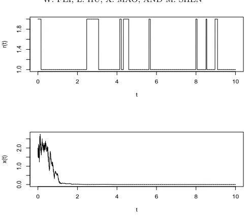
To perform computer simulations, we set\sigma 1= 0.8,\sigma 2= 1.2, and\tau = 0.1 and let the initial data\xi (t) = 2 + sin(t) ont\in [ - 0.1,0] andr(0) = 2. The following computer simulations (Figure 6.1) support our theoretical results clearly.
0 2 4 6 8 10
1
.0
1
.4
1
.8
t
r(t
)
0 2 4 6 8 10
0
.0
1
.0
2
.0
t
x(
[image:23.612.136.379.80.293.2]t)
Fig. 6.1. The computer simulations of the sample paths of the Markov chain and the solution
of (3.9)with the parameters and initial data specified above using the Euler--Maruyama method with step size10 - 3.
6.3. Case 3. In this case we will discuss the robust boundedness. Assume that
(6.19) xTF(x, t, i)\leq ai1 - ai2| x| 2, i\in S1,
and
(6.20) xTF(x, t, i)\leq ai1 - ai2| x| q - p+2, i\in S2,
where all ai1 and ai2 are positive numbers. Suppose that the perturbed system is
described by
(6.21) dx(t) =F(x(t), t, r(t))dt+G(x(t - \tau ), t, r(t))dB(t),
and the perturbation coefficients satisfy
(6.22) | G(y, t, i)| \leq ai3| y| 2, i\in S1,
and
(6.23) | G(y, t, i)| \leq ai3| y| 2+ai4| y| q - p+2, i\in S2,
where ai3 and ai4 are all nonnegative numbers. We aim to obtain upper bounds on
them so that the perturbed system (6.21) remains asymptotically bounded. It follows from these conditions that fori\in S1
xTF(x, t, i) + 0.5(q - 1)| G(y, t, i)| 2
\leq ai1 - ai2| x| 2+ 0.5(q - 1)a13| y| 2,
(6.24)
while fori\in S2
xTF(x, t, i) + 0.5(p - 1)| G(y, t, i)| 2
\leq ai1 - ai2| x| q - p+2+ 0.5(p - 1)ai3| y| 2
+ 0.5(p - 1)ai4| y| q - p+2.
(6.25)
If we compare these with (4.2) and (4.3) in Assumption 4.2, we might attempt to have
\alpha i2= - ai2fori\in S1and 0 for i\in S2.
Consequently, the matrixAdefined by (4.4) becomes
A= diag(pa12, . . . , paN12,0, . . . ,0) - \Gamma .
ButAmight not be a nonsingular M-matrix. To avoid this, we can simply choose a
pair of constants\delta 1>0 and\delta 2\in (0,1) and rearrange (6.25) as
xTF(x, t, i) + 0.5(p - 1)| G(y, t, i)| 2
\leq \alpha i1 - \delta 1| x| 2+ 0.5(p - 1)ai3| y| 2
- (1 - \delta 2)ai2| x| q - p+2+ 0.5(p - 1)ai4| y| q - p+2,
(6.26)
where
\alpha i1= sup
u\geq 0
\bigl(
ai1+\delta 1u2 - \delta 2ai2uq - p+2 \bigr)
.
As a result, Assumption 4.2 is satisfied with
\alpha i1=ai1, \alpha i2= - ai2, \alpha i3= 0.5(q - 1)ai3
fori\in S1 while
\alpha i2= - \delta 1, \alpha i3= 0.5(p - 1)ai3,
\alpha i4= (1 - \delta 2)ai2, \alpha i5= 0.5(p - 1)ai4
for i \in S2 (and \alpha i1 has been defined above). Hence, the matrices A and D in
As-sumption 4.3 become
A= diag(pa12, . . . , paN12, \delta 1, . . . , \delta 1) - \Gamma
and
D= diag(qa12, . . . , qaN12) - (\gamma ij)i,j\in S1.
By Lemma 2.1 and the note below it, bothAand Dare nonsingular M-matrices. In
other words, Assumption 4.3 is satisfied too. To apply Theorem 4.5, we once again choose\beta by (4.8) so condition (4.9) is satisfied by Remark 4.4. Compute\theta i's and\eta i's by (4.6) and (4.7), respectively. Conditions (4.10)--(4.12) then become
(6.27) ai3\leq
2
p(q - 1)\theta i
, ai3<
2\beta
(q - 1)(2q - p)\eta i
fori\in S1
and
(6.28) ai3\leq
2
p(p - 1)\theta i
, ai4<
2q\beta p(p - 1)(2q - p)\theta i
fori\in S2.
By Theorem 4.5, we can therefore conclude that if the perturbed parameters \alpha i3
satisfy (6.15) and (6.16), then for any initial data\xi \in C([ - \tau ,0];Rn), the solutionx(t) of the SDDE (6.21) has properties (4.13) and (4.14).
Example 6.2. Consider a scalar stochastically perturbed hybrid system
(6.29) dx(t) =F(x(t), t, r(t))dt+G(x(t - \tau ), t, r(t))dB(t),
where B(t) is a scalar Brownian, r(t) is a Markov chain with the state space S =
\{ 1,2,3,4\} and the generator
\Gamma = \left(
- 8 1 4 3
1 - 6 2 3
1 1 - 3 1
1 1 0 - 2
\right)
,
and the coefficients are defined by
F(x, t, i) = \left\{
cost - 2x, i= 1,
sint - 3x, i= 2,
cost - 2x3, i= 3,
sint - 3x3, i= 4,
and G(y, t, i) = \left\{
\sigma 1y, i= 1, \sigma 2y, i= 2, \sigma 3y2, i= 3, \sigma 4y2, i= 4.
Let S1 =\{ 1,2\} , S2 = \{ 3,4\} and p= 2, q = 4. It is straightforward to show that conditions (6.19), (6.20), (6.22), and (6.23) are satisfied with
a12= 1.9, a22= 2.9, a32= 1.9, a42= 2.9,
a13=\sigma 12, a23=\sigma 22, a33= 0, a43= 0, a34=\sigma 32, a44=\sigma 42,
andai1's are all positive numbers but their values are of no further use so we do not
specify them. Choose two free parameters\delta 1= 10 and\delta 2= 0.1. Then
A= \left(
11.8 - 1 - 4 - 3
- 1 11.8 - 2 - 3
- 1 - 1 13 - 1
- 1 - 1 0 12
\right)
andD=
\biggl(
15.6 - 1
- 1 17.6
\biggr)
.
Noting that
A - 1= \left(
0.091 0.013 0.030 0.028 0.011 0.089 0.017 0.027 0.009 0.009 0.081 0.011 0.009 0.009 0.004 0.088
\right)
and
D - 1= \biggl(
0.064 0.004 0.004 0.057 \biggr)
,
we see, by Lemma 2.1, that bothAandD are nonsingular M-matrices. We can then
compute
\theta 1= 0.162, \theta 2= 0.144, \theta 3= 0.110, \theta 4= 0.110,
\~
d= 0.068, \~\gamma = 2, \beta = 0.331, \eta 1= 0.023, \eta 2= 0.020.
Conditions (6.27) and (6.28) then become
(6.30) \sigma 1\leq 1.264, \sigma 2\leq 1.356, \sigma 3<1.416, \sigma 4<1.416.
0 2 4 6 8 10
1
.0
2
.0
3
.0
4
.0
t
r(t
)
0 2 4 6 8 10
-0
.5
0
.5
t
x(t
[image:26.612.136.377.93.295.2])
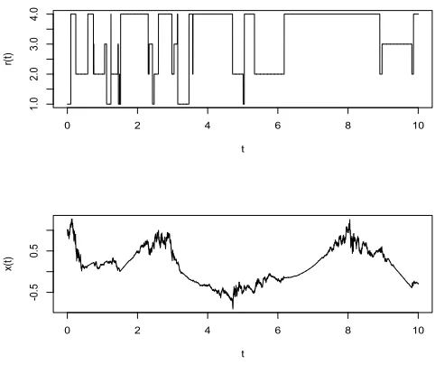
Fig. 6.2. The computer simulations of the sample paths of the Markov chain and the solution
of (6.29)using the Euler--Maruyama method with step size10 - 3.
0 2 4 6 8 10
0
.0
0
.2
0
.4
0
.6
0
.8
1
.0
t
Ex
^2
(t
)
Fig. 6.3. The computer simulation of the second moment of the solution of (6.29)using the
Euler--Maruyama method with step size10 - 3 and sample size 200.
We can therefore conclude that if the perturbed parameters \sigma i satisfy (6.30), then
for any initial data \xi \in C([ - \tau ,0];R), the solution x(t) of the SDDE (6.29) has the properties that
lim sup t\rightarrow \infty
1
t
\int t
0
E| x(s)| 4ds\leq K1,
and
lim sup t\rightarrow \infty
E| x(t)| 2\leq K2,
whereK1 andK2 are positive constants independent of the initial data\xi .
[image:26.612.136.377.335.531.2]