A Novel Method for Extraction of Neural Response from Cochlear Implant Auditory Evoked Potentials

(1)

Theses Thesis/Dissertation Collections

8-2014

A Novel Method for Extraction of Neural

Response from Cochlear Implant Auditory Evoked

Potentials

Daniel Q. Sinkiewicz

Follow this and additional works at:http://scholarworks.rit.edu/theses

This Thesis is brought to you for free and open access by the Thesis/Dissertation Collections at RIT Scholar Works. It has been accepted for inclusion in Theses by an authorized administrator of RIT Scholar Works. For more information, please [email protected].

Recommended Citation

(2)

Response from Cochlear Implant Auditory

Evoked Potentials

by

A Thesis Submitted in Partial Fulfillment of the Requirements for the Degree of Master of Science

in Electrical Engineering

Supervised by

Dr. Behnaz Ghoraani

Department of Biomedical Engineering Kate Gleason College of Engineering

Rochester Institute of Technology Rochester, New York

August 2014

Approved by:

Dr. Behnaz Ghoraani, Assistant Professor

Thesis Advisor, Department of Biomedical Engineering

Dr. Daniel Phillips, Associate Professor

Committee Member, Department of Electrical Engineering

Dr. Sohail Dianat, Department Head - Professor

(3)

Rochester Institute of Technology Kate Gleason College of Engineering

Title:

A Novel Method for Extraction of Neural Response from Cochlear Implant Auditory Evoked Potentials

I, Daniel Q. Sinkiewicz, hereby grant permission to the Wallace Memorial Library to

reproduce my thesis in whole or part.

(4)

c

(5)

Acknowledgments

First and foremost, I would like to thank my advisor Dr. Behnaz Ghoraani for all of her

support during my research. She was a constant source of guidance and experience,

without which this work would never have been possible. I would like to thank Dr. Daniel

Phillips, one of my favorite professors, for serving as one of my committee members,

providing me with a solid foundation in the field of electrical engineering, and providing a

unique perspective on the world. I would also like to thank Dr. Sohail Dianat for serving

as one of my committee members and for developing an excellent curriculum which is the

basis for my success. Additional thanks to Dr. Tsouri, Dr. Patru, Dr. Amuso, Dr. Hoople,

Dr. Hopkins, and Professor Kellerman who, in addition to Dr. Ghoraani and my

committee members, are responsible for teaching me everything I know. Lastly, I would

like to thank my family and friends for their support and patience; you provided me with

(6)

Abstract

A Novel Method for Extraction of Neural Response from Cochlear Implant Auditory

Evoked Potentials

Supervising Professor: Dr. Behnaz Ghoraani

Cortical auditory evoked potential (CAEP) tests are used to evaluate cochlear implant

(CI) patient auditory pathways, but when the CI device processes sound stimuli it produces

an electrical artifact which obscures the relevant information in the neural response.

Cur-rently there are multiple methods which attempt to extract the neural response from the

contaminated CAEP, but there is no gold standard which can quantitatively confirm the

effectiveness of these methods. To address this crucial shortcoming, this work employs

time-frequency analysis, using the continuous wavelet transform (CWT), to quantify how

much artifact energy remains in the neural response recovered by these methods. The

pro-posed CWT evaluation tool calculates the two-dimensional correlation coefficient between

the time-frequency representations of the extracted neural response and the stimulus

sig-nal envelope, which is a good approximation of the artifact, as a means of quantitatively

assessing how much artifact energy remains in the extracted response. A novel technique

for extracting the neural response from contaminated CAEPs is then proposed. The new

method uses matching pursuit (MP) based feature extraction to represent the contaminated

CAEP in a feature space, and support vector machines (SVM) to classify the components

as normal hearing (NH) or artifact. The NH components are combined to extract the

neu-ral response without artifact energy. The proposed method was applied on two sets of CI

CAEPs generated using tone stimuli, and was shown to extract CAEPs from CI data more

effectively than current artifact removal techniques, as verified using the evaluation tool.

The method was then implemented on a CI CAEP generated by a speech stimulus, which

has not been performed by any existing methods, and successfully extracted the neural

re-sponse. The proposed extraction technique and evaluation tool will allow accurate clinical

evaluation of CI patient auditory pathways by removing artifact energy which obscures the

(7)

(8)

List of Tables

4.1 Tone 1 Artifact Correlation Results . . . 30

4.2 Stimulus 1 N1-P2 Latency Results . . . 33

4.3 Tone 2 Artifact Correlation Results . . . 35

4.4 Stimulus 2 N1-P2 Latency Results . . . 38

(11)

List of Figures

2.1 Structure of the Human Ear [15]. . . 5

2.2 Cross Section of the Cochlea [16]. . . 6

2.3 Diagram of an Installed Cochlear Implant Device [18]. . . 7

2.4 Functional Diagram of a Standard Cochlear Implant [5] . . . 8

2.5 Normal Hearing CAEP with Marked N1-P2 Complex [21] . . . 9

2.6 Block Diagram of CIS Speech Encoding Strategy [5] . . . 10

3.1 Coiflet4 Wavelet Function and Scaling Function [27] . . . 16

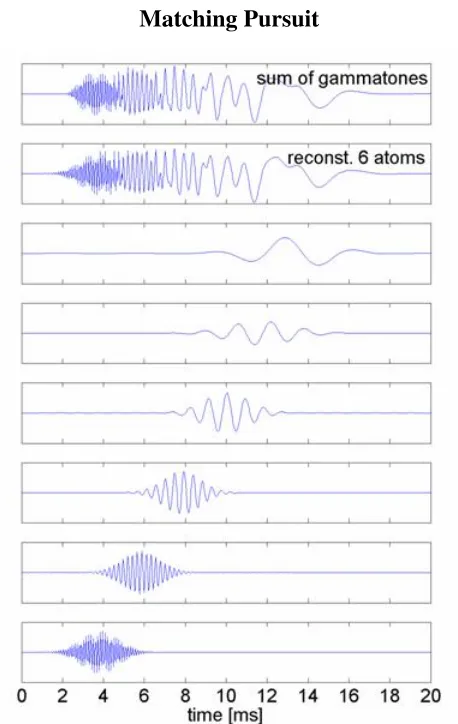
3.2 Example of MP Decomposition. The Bottom Six Plots Show the Atoms Selected to Represent the Signal in the Top Plot. The Second Plot shows the Sum of the 6 Atoms. [29] . . . 18

3.3 Example of Using a Kernel Function to Separate Data in a Higher Dimen-sional Space [30] . . . 19

3.4 Tone 1 (200ms, 1 kHz tone) Stimulus Envelope. A) Time Domain Rep-resentation of Stimulus Envelope B) Time-Frequency RepRep-resentation of Stimulus Envelope. . . 21

3.5 Average NH CAEP Signal for tone 1 in the A) Time Domain and B) Time-Frequency Domain . . . 21

3.6 Example CI CAEP Signal for tone 1 in the A) Time Domain and B) Time-Frequency Domain. CI CAEP has an Artifact Correlation of 0.866. . . 21

3.7 Subtraction Method CAEP Extracted from CI CAEP in Fig. 3.6. A) Time Domain Representation of Signal. B) Time-Frequency Representation of Signal. Recovered CAEP has an Artifact Correlation of 0.658. . . 22

3.8 Polynomial Method CAEP Extracted from CI CAEP in Fig. 3.6. A) Time Domain Representation of Signal. B) Time-Frequency Representation of Signal. Recovered CAEP has an Artifact Correlation of 0.151. . . 23

3.9 CAEP Extraction Technique Block Diagram . . . 23

(12)

3.11 SVM Training and Classification in the Feature Space. A) Artifact and NH NC Components used to Train the NC SVM. B) Artifact and NH PC Components used to Train the PC SVM. C) CI CAEP NC Components Classified as NH or Artifact along with the NC SVM Decision Hyperplane. D) CI CAEP PC Components Classified as NH or Artifact along with the PC SVM Decision Hyperplane . . . 25

4.1 Proposed Method Results for Tone 1 Patient 1. Artifact Correlation De-creased from 0.866 to 0.033 . . . 29 4.2 Proposed Method Results for Tone 1 Patient 2. Artifact Correlation

De-creased from 0.827 to 0.001 . . . 30 4.3 Proposed Method Results for Tone 1 Patient 3. Artifact Correlation

De-creased from 0.837 to 0.081 . . . 33 4.6 Proposed Method Results for Tone 2 Patient 6. Artifact Correlation Changes

from 0.054 to 0.081 . . . 35 4.7 Proposed Method Results for Tone 2 Patient 7. Artifact Correlation

De-creased from 0.373 to 0.061 . . . 37 4.9 Proposed Method Results for Tone 2 Patient 9. Artifact Correlation Changes

from 0.093 to 0.032 . . . 37 4.10 Average NH CAEP for Speech Stimulus. Artifact correlation of 0.001 for

estimated artifact from patient 13. . . 40 4.11 Estimated artifact from patient 13. Taken from channel FT8 and shifted to

match artifact seen on Cz. . . 40 4.12 Proposed Method Results for Speech Patient 10. Artifact Correlation Changes

from 0.093 to 0.077 . . . 41 4.13 Proposed Method Results for Speech Patient 11. Artifact Correlation Changes

(13)

(14)

Chapter 1

Introduction

1.1

Problem and Motivation

Cortical auditory evoked potentials (CAEPs) provide a means of objectively evaluating

neural auditory pathways [1] and potentially speech perception [2]. While CAEPs can be

used to track auditory system maturation in normal hearing (NH) patients, they also provide

a means of assessing sound detection and perception by the hearing impaired, specifically

cochlear implant (CI) patients. The analysis of CI patient CAEPs can provide a means of

ensuring the CI devices are programmed correctly and CI patient auditory pathways are

developing properly. CAEP tests provide a means of noninvasively assessing the

function-ality of the auditory system in CI patients, but an electrical artifact generated by the CI

device currently obscures the relevant information within CI CAEPs.

When a CI device processes a sound and stimulates the cochlea, the device also

gen-erates an electrical artifact shaped like the stimulus signal envelope [3]. A CAEP is

char-acterized by the N1-P2 complex, which consists of a negative peak followed by a positive

peak occurring 100ms and 200ms post-stimulus onset respectively [4]. The stimulus

dura-tion is generally longer than the CAEP, so the artifact obscures the neural response to the

stimulus. The CI device modulates a processed version of stimulus signal envelope onto a

biphasic carrier, which in turn stimulates the auditory nerve [5]. During this process, it is

possible the electroencephalogram (EEG) captures charge collecting on stray capacitance

at the electrode-neuron junction or the electromagnetic fields generated by the stimulating

currents, which produces the artifact. In order to make clinical evaluations of CI patient

(15)

1.2

Purpose of Study

In this work, a tool for evaluating artifact removal techniques is developed along with

a new method for extracting the neural response from a CI CAEP. Currently there are

methods which claim to remove the electrical artifact from CI CAEPs, but the effectiveness

of these methods has not been assessed. There is no gold standard (i.e. a CAEP from

before and after CI device implantation) which can be used to evaluate the artifact reduction

techniques. In order to judge the success of current artifact removal techniques a tool

must be able to separately identify the electrical artifact from the normal CAEP behavior.

The ability to distinguish between neural response and artifact will provide a means to

quantify how much artifact energy remains in an extracted CAEP. A CI CAEP is a

non-stationary process, so the continuous wavelet transform (CWT) can be used to analyze the

CI CAEP in the time-frequency domain [6], where the differences in the artifact and neural

response spectral content will be apparent. This thesis proposes an evaluation tool which

utilizes the CWT to quantitatively assess the success of techniques which extract the neural

response from CI CAEPs. The proposed CWT evaluation tool is the first contribution

towards quantitative assessment of methods for recovering the neural response from CI

CAEPs

A novel technique which combines matching pursuit (MP) and support vector machines

(SVMs) to extract the N1-P2 complex from CI CAEPs is also proposed. MP and SVM

are powerful tools for classifying data samples as either normal or abnormal [9][10]. Most

current applications of these techniques focus only on classifying data in this manner, rather

than extracting desired information from the data marked as abnormal. Instead of using MP

and SVM to classify a signal (i.e. CAEPs) as normal or abnormal, the proposed technique

will be used to extract desired information from an abnormal signal. Most current methods

for extracting the neural response from CI CAEPs attempt to estimate the artifact present in

the signal and subtract it off to recover the neural response. The proposed method attempts

to identify and extract the neural response components within the CI CAEP

1.3

Thesis Organization

This thesis is organized into five chapters.

(16)

the CI device attempts to restore the functionality of the auditory system in hard of

hear-ing subjects. Chapter 2 also describes how CAEPs, which can be used to assess auditory

functionality, are obscured by electrical artifacts generated when the CI device processes

an auditory stimulus. Furthermore, Chapter 2 reviews current methodologies for extracting

the neural response from CI CAEPs.

Chapter 3 (Methods) presents an overview of the background information required to

understand the proposed CWT evaluation tool and artifact extraction technique. This

in-cludes an introduction to the CWT, MP, and SVM. This section then outlines and explains

the CWT evaluation tool implementation and how it is used to assess an extracted CAEP.

Finally, Chapter 3 divides the implementation of the proposed CAEP extraction technique

into three stages, which are discussed individually.

Chapter 4 (Results and Discussion) presents the results of the proposed CAEP

extrac-tion technique, which are assessed using the CWT evaluaextrac-tion tool. The proposed extracextrac-tion

technique was implemented on two sets of CI CAEP data generated using tone stimuli and

one set of CI CAEP data generated using a speech stimulus. The subtraction [13] and

poly-nomial [14] methods for removing the artifact were also implemented on the tone induced

CI CAEPs in order to compare the proposed technique with current methods. For the tone

results, the extracted CAEPs are quantitatively assessed using the CWT evaluation tool and

the N1-P2 complex latencies are used to verify the various methods agree on the extracted

CAEP. The speech CI CAEP results are then analyzed using the CWT evaluation tool to

verify the proposed extraction techniques effectiveness on CAEPs induced with speech

stimuli. Chapter 4 then addresses possible sources of error in the proposed extraction

tech-nique. Additionally, the clinical significance of the presented work is discussed along with

areas for possible improvement within the proposed algorithm.

Chapter 5 (Conclusion) summarizes the work presented in this thesis and provides

(17)

Chapter 2

Background

2.1

Introduction to the Auditory System

The human auditory system is comprised of three stages: the outer ear, the middle ear, and

the inner ear (see Figure 2.1). The outer ear is the only visible part of the auditory pathway,

and its function is to receive and amplify sound waves from the environment. The cartilage

structure around the ear canal, named the pinna, reflects and focuses sound pressure on the

ear canal, which amplifies sounds between 3 and 12 kHz. Covering the end of the ear canal

and separating the outer ear from the middle ear is the tympanic membrane, more

com-monly known as the ear drum. The middle ear is an air-filled cavity which translates the

air pressure waves hitting the tympanic membrane to fluid pressure waves in the cochlea.

Within this cavity are three bones: the malleus, incus, and stapes. When the tympanic

mem-brane vibrates, these bones, called the ossicles, propagate the vibration across the middle

ear to a membrane located on the cochlea, named the oval window. During transmission

of the sound vibrations, the ossicles must increase the pressure of the signal to compensate

for the transition from air to the fluid environment in the cochlea. The primary component

of the inner ear is the cochlea, which translates the mechanical sound waves to electrical

signals for the brain to process. The signal transduction provided by the cochlea makes it

an essential portion of the auditory system.

2.1.1 The Cochlea

The cochlea is shell-shaped structure with three fluid-filled chambers: the scala tympani,

the scala media, and the scala vestibule (see Figure 2.2). When the mechanical vibrations

of the ossicles reach the oval window they produce vibrations in the scala vestibule

(18)

[image:18.612.188.445.114.306.2]

Auditory System Anatomy

Figure 2.1: Structure of the Human Ear [15].

scala vestibule is superior to the scala media, with only the thin Reissners membrane

sepa-rating the two chambers, so vibrations in the scala vestibule pass through the scala media as

well. The fluid in the scala media is endolymph, which is an extracellular fluid containing

a high concentration of potassium ions. Between the scala media and the scala tympani

is the basilar membrane, which acts as a base for the organ of Corti and is displaced by

vibrations in the scala media. The basilar membrane has a frequency selective response

based on the distance from the oval window. This property allows the cochlea to

differ-entiate between sound frequencies, with high frequencies displacing the membrane close

to the oval window and low frequencies displacing the membrane away from the window.

When the basilar membrane moves, microscopic hair cells residing in the organ of Corti are

displaced and depolarized by an influx of potassium ions in the endolymph. When the hair

cells depolarize they trigger action potentials along the spiral ganglion, which eventually

travel along the auditory nerve to the brain.

The auditory pathway is a complex system, where any number of failures can impair

an individuals hearing. Hard of hearing patients can suffer from conductive hearing loss,

where the ossicles or membranes of the outer ear and middle ear do not function correctly,

or sensorineural hearing loss, where the inner ear does not properly transduce mechanical

signals to electrical signals [17]. Sometimes the malfunctions are minor and the patient can

(19)

[image:19.612.183.438.92.316.2]

The Cochlea

Figure 2.2: Cross Section of the Cochlea [16].

enough to overcome the auditory deficiencies. In cases where a component in the auditory

pathway almost completely fails a hearing aid is not enough, because the patient is left

with close to complete hearing loss. As long as the auditory nerve is functioning in these

patients, a cochlear implant (CI) can used to translate acoustic signals to electrical signals

which stimulate the nerve (See Figure 2.3) [5]. In this manner, the malfunctioning part of

the auditory pathway can be skipped and the auditory nerve can be directly stimulated.

2.1.2 Introduction to Cochlear Implants

A CI is a surgically implanted device which mimics the human ear by transducing

mechan-ical sound vibrations to electrmechan-ical signals, which are used to stimulate the auditory nerve. A

standard CI consists of a microphone, a speech processor, a transcutaneous transmitter and

receiver, and a set of up to 22 electrodes placed on the cochlea (see Figure 2.4) [5]. The

mi-crophone picks up sounds from the environment and digitizes them for the CI device. The

external portion of the CI device contains a digital signal processor (DSP), which receives

the digitized sound, extracts the desired features from the signal, and converts the features

into a binary representation for transmission across the skin.

The external unit takes the binary representation of the signal features and transmits

(20)

[image:20.612.187.432.86.325.2]

Cochlear Implant

Figure 2.3: Diagram of an Installed Cochlear Implant Device [18].

The system is designed with a radio frequency (RF) transcutaneous communication channel

because a wired connection passing through the skin would compromise the protection

afforded by skin. The internal unit contains an RF receiver and a stimulator circuit, which

is powered by harvesting energy from the RF transmission. The stimulator interprets the

received bit stream and stimulates the cochlear electrodes accordingly. Modern devices

also contain a feedback loop which monitors the electrical activity of the internal unit [5].

While the feedback loop can ensure the CI device is operating properly, a different test

is required to determine if the device is optimally configured for the patient to hear and

perceive sounds correctly.

2.1.3 CAEPs

Cortical auditory evoked potentials (CAEPs) are measurable changes in the electrical

activ-ity of the brain in response to an auditory stimulus, which can be used as a tool to evaluate

auditory pathways. A typical CAEP consists of multiple electrical events, but the important

event in this application is the N1-P2 complex (see Figure 2.5). The N1-P2 complex

con-sists of a negative peak followed by a positive peak occurring at post-stimulus latencies of

100ms and 200ms respectively [4]. Electroencephalography (EEG) is the technique used

(21)

[image:21.612.196.424.85.273.2]

CI System

Figure 2.4: Functional Diagram of a Standard Cochlear Implant [5]

potentials are a preferable method for assessing a patients physiology because they are

non-invasive. Some of the current clinical uses for CAEPs include assessing hearing in infants

[19] and tracking auditory system maturation in adolescents [1]. CAEPs might be able to

provide a measure of how well individuals can detect and discriminate speech as well [20].

By observing the amplitude and latency of the N1-P2 complex, important information can

be ascertained about a patients auditory development.

CAEPs would be immensely helpful in evaluating the performance and maturation of

auditory systems in patients with CI devices. The results of these tests would help ensure

the devices are programmed correctly for each patient and could provide insight into the

patients ability to perceive speech correctly. When CI devices process the auditory

stim-ulus and stimulate the auditory nerve, they also generate a large electrical artifact which

obscures the CAEP in EEG recordings. Removing the electrical artifact generated by the

CI device is crucial to evaluating CI patients using noninvasive evoked potentials.

2.1.4 Electrical Artifact

In EEG recordings of CI CAEPs a large electrical artifact obscures the N1-P2 complex,

preventing clinical analysis of the data. The artifact morphology has been shown to closely

follow the shape of the stimulus signal envelope [3]. One study used a high-sample-rate

acquisition system to better understand the artifact, and the results showed the artifact

con-sisted of the stimulus envelope modulated on top of a high frequency carrier [13]. These

(22)

[image:22.612.175.431.88.269.2]

CAEP

Figure 2.5: Normal Hearing CAEP with Marked N1-P2 Complex [21]

stimulation. Modern CI devices only extract and encode the coarse features of a sound,

such as the temporal envelope. The temporal envelopes from a limited number of

spec-tral bands have been shown to produce a high level of speech recognition for a given

sound sample [22]. This idea is the basis for a popular method of speech processing called

continuous-interleaved-sampling (CIS), which is still used in modern CI devices to extract

coarse features from speech (see Figure 2.6) [5].

The CIS strategy employs a band pass filter for each electrode implanted on the cochlea.

These filters break the signal into spectral bands, and for each band the temporal envelope

of the filtered signal is obtained. Two methods commonly used to generate the envelopes

are full wave rectification followed by a low pass filter and, more recently, using the Hilbert

transform [5]. These signals cannot be directly applied to the cochlea though, because the

electrical dynamic range of the cochlea is much smaller than the dynamic range of speech

amplitudes. Human speech can have an acoustic dynamic range of 30-50dB, which must be

compressed down to a patients electrical dynamic range of about 5dB [23]. The temporal

envelopes are logarithmically compressed using a function such as the power-law function:

Y =Axp+B (2.1)

WhereAandBare patient specific constants, andpis a variable between 0 and 1 which

controls the steepness of the compression function [23]. The compressed envelopes then

amplitude modulate biphasic pulse carriers, which are used to stimulate the cochlear

(23)

electrodes, which can lead to electromagnetic field (EMF) interference between electrodes

and corruption of the signals [5]. The artifact may be the result of charge from these

stim-ulation signals building up on stray capacitances at the electrode neuron junction. Another

possibility is the EEG electrodes detect the EMF generated by the stimulating currents. In

either case, as long as the current stimulation strategy is employed the electrical artifact

will contaminate CI CAEPs.

[image:23.612.162.456.205.394.2]

CIS Strategy

Figure 2.6: Block Diagram of CIS Speech Encoding Strategy [5]

2.2

Review of Current Methodologiess

There are currently three main approaches for removing CI electrical artifacts from CAEPs:

the subtraction method, the polynomial method, and ICA based algorithms.

2.2.1 Subtraction Method [13]

The subtraction method takes advantage of the neural refractory period to produce an

es-timate of the electrical artifact. The N1-P2 response amplitude is dependent on the

inter-stimulus interval (ISI), which is the length of time between the offset of the previous

stim-ulus and the onset of the next stimstim-ulus. The N1-P2 complex amplitude increases with

increasing ISI length up to a peak amplitude, which is achieved at an ISI of 10 seconds

or greater [24]. When the ISI is on the order of 500ms the N1-P2 complex amplitude is

(24)

by the CI device, which performs the same regardless of the ISI length. CAEPs generated

with small ISIs are dominated by the electrical artifact, making them a good estimate of

the artifact under the specific recording conditions used. By taking two CAEP recordings

from a patient, one with a small ISI and one with a large ISI, the small ISI CAEP can be

used as an estimate for the artifact in the large ISI CAEP. This method is a straight forward

technique, requiring only two CAEP recordings on one electrode to produce a clean signal

for that specific channel. The estimated artifact still contains some neural response though,

so subtracting it from the large ISI CAEP removes additional neural response energy

be-yond the artifact. Since the method requires recording two sets of CAEPs, any changes the

artifacts shape between the two sets can produce inaccurate results. If the EEG cap were to

shift between tests, then the artifact shape could change and the estimated artifact may not

completely remove the artifact form the CI CAEP.

2.2.2 Polynomial Method [14]

The polynomial method uses the recorded CI CAEP along with the stimulus envelope to

estimate the artifact using a polynomial function. This method models the artifact as a

bi-variate polynomial based on both time and the stimulus envelope. The polynomial is fit to

the CAEP using the textitpolyfitn MATLAB function, with time and the stimulus envelope

as the independent variables and the CAEP as the dependent variable. The polynomial is

limited to 3rd, 4th, or 5th order, and the polynomial fitting process is constrained to the

known location of the artifact. In order to prevent the polynomial from fitting the neural

response in addition to the artifact, the CI CAEP within the constrained fit is randomized

first. This process preserves the statistical features of the CAEP. This technique only works

on tone stimuli, because the stimulus envelope of a tone is not time varying and will not be

affected by this randomization. CAEPs generated using speech stimuli cannot be

random-ized in the same way, because the polynomial must be fit to the time-dependent stimulus

envelope within the CI CAEP. In this case, the polynomial will fit both the artifact and the

neural response, which means subtracting the polynomial from the CI CAEP will not yield

the neural response. While tones stimuli are useful because they can generate CAEPs,

nat-urally produced speech stimuli are more representative of everyday speech and can provide

more insight into CI patient speech perception. The polynomial representation of the

ar-tifact for a tone induced CAEP can be subtracted from the CI CAEP to extract the neural

(25)

requires one data set to implement, but it is limited to data generated from tone stimuli.

2.2.3 ICA Based Algorithm [12][25]

Independent component analysis (ICA) is a blind source separation technique which is

applied to CI CAEPs to recover the original neural response and electrical artifact. The

primary assumption behind ICA is the chosen signal is a combination of statistically

inde-pendent sources, but the artifact and CAEP are time locked to the stimulus and therefore not

completely independent. This lack of true independence can lead to neural energy being

erroneously removed with the artifact, or artifact energy being left in the recovered CAEP.

According to the central limit theorem, combining independent signals will make a mixed

signal with a more Gaussian distribution than the individual signals had. This means

cor-rectly removing sources would make the mixture less Gaussian. ICA estimates independent

components by finding the signal which, when removed, maximizes the non-Gaussianity

of the remaining mixed signal. ICA will not produce the original neural response and

arti-fact, but rather a set of independent components which can be combined into the response

and artifact. The artifact has been shown to consist of multiple independent components

that must be manually identified and removed by a trained individual. ICA algorithms

usually whiten the data and implement principle component analysis (PCA) to reduce the

dimensionality of the data before applying ICA. This pre-processing causes ICA to produce

slightly different independent components each time it is implemented on the same data set.

ICA also requires more observation points than independent components, necessitating the

use of multichannel EEG data.

There is currently no gold standard against which to compare the results produced by

these methods though. While these techniques may visually appear to remove the artifact,

they have not been tested on a data set containing CAEPs from before and after a patient had

a CI device. Visual inspection cannot definitively confirm whether the neural response was

completely extracted from the CI CAEP, which means the effectiveness of these methods

(26)

Chapter 3

Methods

3.1

Data Collection

Three different types of stimuli were used to collect data from CI subjects: a short tone,

a longer tone, and a speech stimulus. The tone stimuli were used to generate two sets

of CAEP data, one set with 500ms ISIs and one set with 3000ms ISIs. The tests with

different ISIs were used to accommodate the subtraction method, which approximates the

artifact as the short ISI CAEP. The 3000ms ISI CAEPs were used to test the polynomial and

proposed methods. While tone stimuli are useful because they can induce a CAEP, speech

stimuli are much more representative of everyday spoken language. CAEPs generated

using speech stimuli can provide a better insight into how CI patients discern and perceive

everyday speech. Spoken words also have much more complex stimulus envelopes than

tones, which means the electrical artifact generated by a speech stimulus is much more

difficult to remove. The proposed artifact removal technique was first tested on CI CAEPs

generated using tone stimuli to verify its effectiveness, and then it was implemented on

speech CI CAEPs to ensure the method extracts the CAEP regardless of the stimulation

source.

3.1.1 Tone 1

Subjects: The subjects for tone 1 consisted of 5 CI patients (54-77 years old) with

Ad-vanced Bionics HiRes 90K CI devices. All patients were native English speakers with no

history of neurological disorders.

Stimulus: The stimulus was a 200ms pulse train, with biphasic pulses of 57us per

phase, generated at 1 kHz. Two homogeneous blocks of 200 instances of the stimuli

with inter-stimulus intervals (ISI) of 500ms or 3000ms were presented directly to the

(27)

BEDCS research interface.

Electrophysiological Testing: A Neuroscan data collection system with a 65

chan-nel electrode cap was used to collect the CAEP recordings. Unless otherwise stated, all

analyzed CAEPs were taken from the Cz electrode.

3.1.2 Tone 2

Subjects:The subjects consisted of 4 CI patients (50-55 years old) with Advanced Bionics

HiRes 90k CI devices and 7 NH patients (50-53 years old). All patients were native English

speakers with no history of neurological disorders.

Stimulus: The stimulus was a 656 ms biphasic current pulse train with pulse duration

of 20 us and a pulse rate of 1000 kHz. Two homogeneous blocks of 350 instances of

the stimuli with 500ms or 3000ms ISIs were presented directly to the subjects’ CI at their

MCL, bypassing the speech processor.

Electrophysiological Testing: A Neuroscan data collection system with a 65 channel

electrode cap was used to collect the CAEP recordings.

3.1.3 Speech

Subjects: Subjects consisted of 4 NH individuals (23-31 years old) and 5 CI users (37-57

years old) with Nucleus-24 CI devices. All patients were native English speakers with no

history of neurological disorders.

Stimulus:The stimulus for all subjects was the syllable ’shi’ (656 ms duration), spoken

by a female reader, taken from the ”Nonsense Syllable Test” [26], presented in the sound

field at 65 dB HL for 300 instances.

Electrophysiological Testing: A Neuroscan data collection system with a 32 channel

electrode cap was used to collect recordings.

3.2

Methodology Background

3.2.1 Continuous Wavelet Transform

The CWT is a method for representing a signal in the time-frequency domain, where

fre-quency content can be localized in time [6]. Traditional Fourier analysis maps a signal to

(28)

frequencies. These sinusoids are infinite in duration though, so the frequency content of a

signal cannot be localized to a specific time. In a non-stationary process (i.e. a CI CAEP

signal) the spectral properties of the signal are dependent on time and it is often desirable

to locate a specific set of frequencies, such as the electrical artifact spectral content, in the

time domain. The CWT achieves a time-frequency representation by decomposing a

sig-nal into a summation of finite length wavelets of different scales instead of infinite length

sinusoids with different frequencies.

The wavelets are dilated, or scaled, and shifted versions of the same mother wavelet

(MW). The scaling of the wavelet in the time domain determines what frequency the

wavelet corresponds to, with large scale values corresponding to low frequencies and vice

versa. The MW is shifted in position, b, along the chosen signal while maintaining a

con-stant scale value to determine the contribution of the scale to the overall signal. The MW is

then dilated by a scaling factor, a, and shifted along the signal to determine the contribution

of the new scale to the signal. This process is repeated over a desired range of scale values,

and can be mathematically described by Equation 3.1:

T(a, b) = √1 a

Z ∞

−∞

x(t)ψ∗(t−b

a ) dt (3.1)

where

ais the scaling factor of the wavelet.

bis the position of the wavelet.

x(t)is the original signal.

ψ∗(t)is the complex conjugate of the MW function.

The scale factor allows the CWT to localize a signal in the frequency domain, while

the MWs finite length and position allow for time localization. The range of scale values

used during the analysis of CI CAEPs was selected based on the frequency content of the

CAEPs. Fourier analysis determined CI CAEP frequency content is limited to the range

of 1-50Hz. Wavelet scale values do not correspond directly to frequency, but rather to

pseudo frequencies. These pseudo frequencies are calculated using the center frequency of

the chosen MW. For this analysis, the Coiflet4 MW [27] (see Figure 3.1) was found to be

suitable and the frequency range of 1-50Hz was translated to scale values according to this

(29)

The CWT also uses a Father Wavelet (FW), called the scaling function, to handle

spec-trum the MW cannot fully cover. In order to handle all frequency values down to zero, an

infinite number of MWs with increasing scale values would be necessary. Instead, the FW

is designed with a low-pass spectrum to cover this frequency range. The FW can then be

decomposed using the MW and the signal can still be fully represented using the MW [28].

This strategy allows the CWT to cover the entire spectrum using a finite number of MWs.

[image:29.612.111.512.224.393.2]

Coiflet4 Wavelet

Figure 3.1: Coiflet4 Wavelet Function and Scaling Function [27]

3.2.2 Matching Pursuit

Matching Pursuit (MP) is a process in which a signal is approximated using a redundant

dictionary of atoms,g [7] (see Figure 3.2). Multiple types of atoms, such as pure sinusoids

or MWs, can be used to construct a dictionary. For reference, the CWT can be written

in terms of MP with a dictionary constructed from scaled and shifted versions of a single

MW. MP differs from the Fourier transform and CWT because it can decompose a signal

using different shaped basis functions, rather than uniformly shaped basis functions. The

basic MP algorithm projects the chosen signal onto all the atoms in a dictionary and selects

the atom which produces the maximum absolute inner product with the signal. Out of the

entire dictionary, the chosen atom matches the current signal the best. The atom is scaled

by this inner product and subtracted from the signal to produce a residual,R. One iteration

(30)

Rnx=< x, gγn > gγn+R

n+1_x _(3.2)

where

Rnxis thenth order residual.

xis the original signal.

gγn is the is the atomnin the family gamma.

Rn+1_x_{is the new residual generated from approximating}_x_{in the dimension}_g

γn.

For the first iteration, R0_x _{is defined as}_x_{. This expression is repeated on the residual}

signal generated during subsequent iterations until the desired algorithm stopping criterion

is met. For this application, the stopping criterion was chosen to be a fixed number of

iter-ations. After an experimentally determined number of MP iterations, the subsequent

com-ponents contribute negligible energy to the original signal and can therefore be excluded

without losing information. This expression for a MP signal approximation is shown in

Equation 3.3:

x=

M−1

X

n=0

< Rnx, gγn > gγn+R

M_x

(3.3)

where

xis the original signal.

M is the current number of iterations.

nis the current iteration number.

RM_x_{is the}_M_{th order residual.}

The basic MP algorithm used to decompose CAEPs is not orthogonal, so the same atom

is placed back in the dictionary and can be used multiple times. The basis functions chosen

by the MP algorithm and their weights can be thought of as components of the original

signal. These components can be plotted into a feature space based on their properties,

such as scale, position and energy, to further analyze the signal.

During MP implementation, a dictionary of atoms was constructed in MATLAB and

(31)

[image:31.612.195.424.85.447.2]

Matching Pursuit

Figure 3.2: Example of MP Decomposition. The Bottom Six Plots Show the Atoms Selected to Represent the Signal in the Top Plot. The Second Plot shows the Sum of the 6 Atoms. [29]

3.2.3 Support Vector Machines

Support vector machines (SVMs) are binary classification models which use supervised

learning to determine which category, out of two, new data points fall in. SVMs are initially

trained using examples of data whose category is known. Based on this training sequence,

the SVM will classify new data points as falling into one of the two categories. SVM uses

the training sequence to generate a hyperplane in the data feature space, with each side of

the hyperplane representing a class. When the data is non-separable (i.e. a hyperplane will

not perfectly separate the data) a penalty variable,C, is introduced which places restrictions

on how tolerant of misclassifications the model is [8]. The best hyperplane is chosen to

(32)

generalization errors when new data points are presented to the model.

[image:32.612.128.491.114.295.2]

SVM Kernel Function

Figure 3.3: Example of Using a Kernel Function to Separate Data in a Higher Dimensional Space [30]

When data cannot be easily separated by a hyperplane in the current feature space, the

data can be mapped to a higher dimensionality where it can be separated (see Figure 3.3).

This remapping is performed using a kernel function. When the SVM training algorithm

searches for the optimal hyperplane, it only uses the dot product to operate on the training

data sets. This is advantageous because the algorithm does not have to remap all data

points to this higher dimensional space. The algorithm only has to compute the dot product

between two of the data points in that space. In this scenario, the kernel only needs to

be used in the training sequence to determine the hyperplane, which can then be brought

back to the original feature space [8]. The kernel trick allows the data to be analyzed in a

higher dimensional space without requiring the explicit remapping of all the data and does

not significantly change the computation time of the model. For this analysis, the Gaussian

radial basis function (RBF) kernel was used because it is a flexible kernel which was found

to fit the CAEP data in the features space well. The formula for the Gaussian RBF can be

seen in Equation 3.4:

K(x, y) = e

−kx−yk2

2σ2 (3.4)

where

xis one data point.

(33)

σ is a parameter which controls the overall shape of the SVM hyperplane.

The MATLAB functions textitsvmtrain and textitsvmclassify were used to respectively

train and classify SVMs using the RBF kernel.

3.3

Proposed Tool for Artifact Removal Evaluation

In order to evaluate how well a technique removes the electrical artifact from contaminated

CAEPs, the CAEPs from before and after the artifact removal were analyzed using the

CWT and the correlation function. The artifact shape is directly related to the signal

en-velope of the stimulus, so the CWT of the stimulus enen-velope provides a good estimate of

the artifacts spectral energy. The stimulus envelope of Tone 1 is shown in Fig. 3.4A and its

corresponding time-frequency representation is shown in Fig. 3.4B. In this representation,

the x-axis denotes time, the y-axis denotes frequency, and the color scale denotes

coeffi-cient magnitudes. Coefficoeffi-cient magnitudes are used instead of their signed values because

the representation is meant to convey the spectral energy of the signal. A NH CAEP can

be seen in Fig. 3.5A along with its time-frequency representation in Fig. 3.5B, and a

con-taminated CAEP can be seen in Fig. 3.6A along with its time-frequency representation in

Fig. 3.6B. The artifact, as seen in Fig. 3.4B, can clearly be seen in the CI CAEP

time-frequency plot. By comparing the stimulus envelope time-time-frequency plot to the CI CAEP

before and after artifact removal, the removal process can be evaluated. The magnitude

of the correlation coefficient between a stimulus envelope and its corresponding CAEP in

the time-frequency domain is called the artifact correlation, and it can assess the artifact

removal process. A large artifact correlation for an extracted CAEP can indicate there is

either still artifact energy in the neural signal or CAEP energy was removed with the

arti-fact. The artifact correlation of the average NH CAEP was 0.045, which indicates a small

artifact correlation corresponds with little residual artifact energy.

To determine how successfully the subtraction and polynomial methods, outlined in

[13] and [14] respectively, remove the artifact, the methods were assessed using the

pro-posed CWT evaluation tool. Both methods were implemented on the CI CAEP from tone 1,

shown in Fig 3.6. Fig. 3.7A shows the CAEP extracted by the subtraction method and Fig.

3.7B shows its corresponding time-frequency plot. The resulting CAEP clearly contains

(34)

[image:34.612.100.528.96.236.2] [image:34.612.98.529.295.434.2]

Figure 3.4: Tone 1 (200ms, 1 kHz tone) Stimulus Envelope. A) Time Domain Representation of Stimulus Envelope B) Time-Frequency Representation of Stimulus Envelope.

Figure 3.5: Average NH CAEP Signal for tone 1 in the A) Time Domain and B) Time-Frequency Domain

[image:34.612.99.536.493.632.2]

(35)

of 0.658. For reference, the original CI CAEP produced an artifact correlation of 0.866.

While the subtraction technique did remove the artifact completely for some patients, it

still left behind energy from the artifact for other patients. This remaining artifact energy

can only be observed using the CWT. Visually, the subtraction method appears to have

extracted what could be the neural response from the CI CAEP, but the evaluation tool

identifies artifact energy in the extracted CAEP. In comparison, the time-frequency

anal-ysis of typical polynomial method results can be seen in Fig. 3.8. The clean CAEP can

be seen in Fig. 3.8A, while its corresponding time-frequency analysis can be seen in Fig.

3.8B. This time-frequency plot produced an artifact correlation of 0.151. The polynomial

method removed most of the artifact spectral energy for this example CI CAEPs produced

by tone 1.

Figure 3.7: Subtraction Method CAEP Extracted from CI CAEP in Fig. 3.6. A) Time Domain Representation of Signal. B) Time-Frequency Representation of Signal. Recovered CAEP has an Artifact Correlation of 0.658.

The proposed evaluation tool provides a quantitative assessment of how successful an

artifact removal process is, along with a graphical representation of what artifact energy

remains in the extracted CAEP.

3.4

Proposed Method for CAEP Recovery

The proposed extraction method is a novel technique which combines MP based feature

extraction with SVM binary classifiers to identify and recover the NH components within

a CI CAEP. A block diagram of the proposed method for extracting the N1-P2 complex is

(36)

Figure 3.8: Polynomial Method CAEP Extracted from CI CAEP in Fig. 3.6. A) Time Domain Representation of Signal. B) Time-Frequency Representation of Signal. Recovered CAEP has an Artifact Correlation of 0.151.

Figure 3.9: CAEP Extraction Technique Block Diagram

3.4.1 MP Feature Extraction

MP is implemented on the signals using a redundant dictionary constructed from Gabor

functions, which are generated using the following equation [31]:

G= √1 se

−π(n−u)2

s2 cos(2πω(n−u) +θ) (3.5)

where

Gis the Gabor function.

sis the scale factor of the function.

(37)

ω is the normalized frequency.

θ is the phase of the function.

For this analysis, the Gabor atoms were constructed by varying the scale factor from

1 sample to the length of the signal, N, for normalized frequency values of 0 and 0.001.

The phase was set to 0 for all Gabor functions. The stopping criterion was experimentally

determined to be 40 iterations for data from tones 1 and 2 based on the coefficient values

produced after each MP iteration. The coefficient magnitudes, which were first normalized

to the first coefficient value, were less than 0.6% after the 40th iteration, as shown in Fig.

3.10, and therefore contribute little energy to the original signal. The components produced

by the MP algorithm were plotted in a three dimensional feature space, with the three

[image:37.612.146.472.335.493.2]

dimensions representing position, scale (as a power of two), and coefficient.

Figure 3.10: MP Coefficients Produced over 60 Iterations for Tone 1 CI CAEP

3.4.2 SVM Training

The estimated artifact and average NH CAEP are decomposed using MP to generate

train-ing data sets. These components are used by SVM to generate a hyperplane which can

separate NH and artifact components. The artifact and NH CAEP components generated

by the MP algorithm are not perfectly separable in the current feature space, so an RBF

kernel function is used to create a hyperplane which will provide more accurate

classifica-tion. Prior to SVM training, the logarithm of the component coefficient magnitudes was

(38)

coefficients led the SVM to classify negative peaks from the CAEP incorrectly though, so

in order to retain the coefficient sign the data is split up into two sets: one for components

with positive coefficients (PC) and one for components with negative coefficients (NC).

Figs. 3.11A and 3.11B show an example of artifact and NH training components plotted in

the feature space.

Figure 3.11: SVM Training and Classification in the Feature Space. A) Artifact and NH NC Com-ponents used to Train the NC SVM. B) Artifact and NH PC ComCom-ponents used to Train the PC SVM. C) CI CAEP NC Components Classified as NH or Artifact along with the NC SVM Decision Hyperplane. D) CI CAEP PC Components Classified as NH or Artifact along with the PC SVM Decision Hyperplane

The SVMs use two parameters to control the shape of their decision hyperplanes. The

Gaussian RBF kernels contain a free parameter, σ, which controls the overall shape the

hyperplane takes, with high values producing a smoother hyperplane and low values

pro-ducing a more variable hyperplane. This parameter is similar to the standard deviation

of a normal Gaussian distribution, where a large standard deviation produced a smoother

curve and a small standard deviation produces a sharper curve. The second parameter is the

penalty term, C, which controls the acceptable degree of misclassification [8]. These

pa-rameters determine how closely the SVM fits the hyperplane to the training data. If the

hy-perplane over-fits or under-fits the training data, then the SVM loses generalization and new

(39)

for each patient is determined by implementing a grid search over possible combinations of

these two parameters [32], and applying the CWT evaluation tool to the recovered CAEP

from each combination. For each patient, the combination which generates the CAEP with

the lowest artifact correlation is selected. CAEPs can vary significantly between patients

and recording sessions, so different combinations of σ and C will produce hyperplanes

which fit different signals better.

3.4.3 SVM Classification and CAEP Extraction

After training, the SVM hyperplanes are used to classify the CI CAEP components as either

artifact or neural response. Figs. 3.11C and 3.11D show an example of classified CI CAEP

components plotted in the feature space along with hyperplane surfaces for both SVMs

for one subject. The NH components are taken from each SVM and summed together to

produce the extracted CAEP.

3.5

Summary

This chapter outlines the methodology behind the CWT evaluation tool and the novel

tech-nique for extracting the CI CAEP. The CWT evaluation tool requires the stimulus envelope

and extracted CAEP to produce a quantitative assessment of the artifact energy remaining

in the neural response. The tool calculates the two-dimensional correlation coefficient

be-tween the time-frequency representations of both signals to estimate how much residual

artifact energy is present in the extracted CAEP. The novel technique for extracting the

neural response from the CI CAEP using MP and SVM is then outlined. The stimulus

en-velope and average NH CEAP are decomposed using MP with Gabor functions and passed

to the SVMs as training data. The SVMs use Gaussian RBF kernels and a grid search

to determine the optimal parameters for a given CI CAEP. The CI CAEP is then

decom-posed using MP and the components are classified as either artifact or neural response by

the trained SVMs, and the neural response components are combined to extract the CAEP.

This methodology describes the steps which can be followed to implement the proposed

evaluation tool and CAEP extraction technique to produce the results reported in Chapter

(40)

Chapter 4

Results and Discussion

The purpose of this chapter is to present figures and tables which demonstrate the

perfor-mance of the proposed artifact extraction technique and CWT evaluation tool. In Section

4.1, the proposed method was implemented on CI CAEPs from tone 1. Section 4.2

con-tains the results from applying the proposed method on tone 2 CI CAEPs. For both tone

CI CAEPs, the subtraction and polynomial methods were also applied to data for

compari-son. The results of each method were assessed using the CWT evaluation tool to determine

how effectively each method extracted the CAEP. Section 4.3 applies the proposed CAEP

extraction technique on CI CAEPs generated using speech stimuli, which have complex

artifacts current methods cannot remove. In Section 4.4, sources of error for both the CWT

evaluation tool and the proposed CAEP extraction technique are considered and analyzed.

Section 4.5 addresses the practical and clinical significance of the proposed work, including

its advantages over current methods for extracting the neural response from CI CAEPs. In

particular, the proposed CWT evaluation tool is the first contribution towards quantitative

assessment of methods for removing the artifact from CI CAEPs. Possible improvements

to the CWT evaluation tool and CAEP extraction technique are also outlined in Section 4.6.

4.1

Tone 1

The proposed artifact removal technique was applied to five CI patients from the tone 1 test

group. The subtraction and polynomial methods were also applied to this data to compare

the proposed method with current CAEP extraction techniques. All results were analyzed

using the CWT evaluation tool to assess how successfully each method extracted the neural

(41)

4.1.1 Data Analysis Procedure

The following procedure outlines the process of applying the proposed CAEP extraction

technique to the CI CAEP data.

• The MP algorithm was used to decompose the normalized 200ms, 1 kHz stimulus envelope and normalized average NH CAEP to create artifact and NH CAEP training

components respectively. The MP stopping criterion was set to 40 iterations, resulting

in a total of 80 training components.

• The training components were conditioned and passed to the SVMs. The condition-ing consisted of splittcondition-ing the components into two groups: positive coefficients and

negative coefficients. The logarithm function is then applied to the magnitude of the

coefficients for each group in order to further spread out the components. Both the PC

and NC SVMS used RBF kernel functions to generate the appropriate hyperplanes.

The optimal SVM parameter grid search for tone 1 was experimentally determined to

cover ofσ∈(0.3, 0.5) andC∈(0.01, 0.1, 1, 10, 100).

• For each patient, the SVMs were trained for all ten combinations of SVM parameters and the CWT evaluation tool was used to select the pair which generated the CAEP

with the lowest artifact correlation. The grid search is fully automated, and can be

expanded to include more values of and C at the expense of computation time. To

keep the search from becoming unwieldy, the same parameters were used in the PC

and NC SVMs.

• After the optimal parameters were selected for a given patient, the SVMs were trained

with the chosen parameters and used to classify the CI CAEP components. The NH

components were combined to extract the neural response from the CI CAEP.

4.1.2 Tone 1 Results

The proposed method extracted clear N1-P2 complexes from all five CI CAEPs analyzed

for tone 1. These results were assessed using the CWT evaluation tool. Fig. 4.1 shows the

results of the CAEP recovery process for subject 1 of tone 1. Figs. 4.1A and 4.1B show

the original CI CAEP and its corresponding time-frequency plot respectively, while Figs.

4.1C and 4.1D show the recovered CAEP and its corresponding CWT respectively. The

(42)

compares favorably with the NH response of Fig. 3.5B. The CWT evaluation tool measured

the extracted CAEP artifact correlation at 0.033. For reference, the CI CAEPs from tone 1

have an average artifact correlation of 0.840. Based on these results, the recovered CAEP

[image:42.612.100.522.176.430.2]

contains almost no spectral energy introduced by the artifact.

Figure 4.1: Proposed Method Results for Tone 1 Patient 1. Artifact Correlation Decreased from 0.866 to 0.033

Figures 4.2 through 4.5 contain the CI CAEPs from patients 2 through 5 before and

after the proposed extraction technique was applied.

Table 4.1 contains the CWT evaluation of the results obtained from applying the

pro-posed method, the subtraction method and the polynomial method on the tone 1 CI CAEPs.

The subtraction method produced an average artifact correlation of 0.344, suggesting

ar-tifact energy remains in CAEPs extracted using this technique. The polynomial method

produced and average artifact correlation of 0.150. These results indicate the polynomial

method extracts a cleaner CAEP, on average, than the subtraction method. The proposed

method produced an average artifact correlation of 0.024, leaving almost no artifact

com-ponents in the recovered CAEPs.

The CWT evaluation tool provides insight into how the methodology behind each

(43)

[image:43.612.99.528.98.345.2]

Table 4.1: Tone 1 Artifact Correlation Results

Patient CI CAEP Proposed Subtraction [13] Polynomial [14]

1 0.866 0.033 0.658 0.151

2 0.827 0.001 0.140 0.120

3 0.817 0.001 0.140 0.209

4 0.851 0.004 0.137 0.127

5 0.837 0.081 0.643 0.144

Combined 0.840±0.017 0.024±0.031 0.344±0.251 0.150±0.031

correlation generated by the subtraction method results appears to indicate the method does

not extract a particularly clean neural response from CI CAEPs, but the individual

pa-tient results suggest otherwise. For papa-tients 2 through 4, the subtraction method produced

CAEPs with low artifact correlations, which are comparable to the polynomial method

re-sults for the same patients. The average subtraction rere-sults are skewed by patients 1 and 5,

which contained large amounts of artifact energy in the extracted CAEP. The inconsistency

of the subtraction method can be seen in the standard deviation of its results, which is eight

times larger than the standard deviations for the polynomial and proposed methods. These

results demonstrate the primary flaw in the techniques methodology. The subtraction

(44)

[image:44.612.108.525.96.341.2]

CAEP with a long ISI for the same patient. This is a reasonable assumption if both sets

of CI CAEPs are taken during the same test and have the same recording conditions. If an

element of the recording process changes, such as the EEG electrode cap shifting, the

arti-fact present in the short ISI CI CAEP will differ from the artiarti-fact in the long ISI CI CAEP.

When the incorrect artifact is subtracted from the long ISI CI CAEP, artifact energy will

remain in the resulting neural response. While the subtraction method works comparably

to the polynomial method when the short ISI CI CAEP provides a good estimate of the

artifact, the need for a second recording introduces a source of error which can reduce the

effectiveness of the method.

The polynomial method produces much more consistent results than the subtraction

method, but they are still relatively large with a mean artifact correlation of 0.150. The

polynomial method fits a polynomial to the stimulus envelope and the CI CAEP in order

to estimate the artifact present in the CI CAEP. The CWT evaluation tool results indicate

the polynomial method might be over fitting the CI CAEP though, removing neural energy

in the process. The actual correlation coefficients between the polynomial results and the

(45)

[image:45.612.97.519.98.340.2]

negative correlation with the stimulus envelope. This negative correlation is caused by

additional energy being removed from the CAEP beyond just the artifact energy, creating

an absence of neural energy where the artifact spectral energy once resided. While the

artifact is completely removed from the resulting CAEP, the N1-P2 complex amplitude

might be affected by the missing neural energy.

The proposed method produces the lowest average artifact correlation out of all tested

methods. This novel technique makes use of MP and SVM to individually identify the

CI CAEP signal components as either neural response or artifact, and selectively extracts

the neural response components. The subtraction and polynomial techniques attempt to

estimate the artifact within a CI CAEP and subtract it off, while the proposed method

identifies neural response components present within the CI CAEP and extracts them. This

approach, on average, extracts CAEPs with very low levels of residual artifact energy.

4.1.3 N1-P2 Latency

In order to verify the applied methods agree on the extracted CAEPs for tone 1, the peak

(46)

[image:46.612.99.520.97.340.2]

Table 4.2: Stimulus 1 N1-P2 Latency Results

N = 5 Proposed Subtraction [13] Polynomial [14]

N1 (ms) 122±8 122±4 121±10

P2 (ms) 197±7 207±15 200±3

by a negative peak occurring 100ms post-stimulus, followed by a positive peak occurring

200ms post-stimulus. Table 4.2 contains the tone 1 N1-P2 complex latencies as determined

by the various artifact removal techniques. All three methods show good agreement with

the literature on the latencies of the N1 and P2 peaks, placing them around 120ms and

200ms respectively. This agreement indicates all three methods did indeed recover the

N1-P2 complex from the CI CAEPs.

4.2

Tone 2

The proposed artifact removal technique was applied to four CI patients from the tone 2

test group. As with the tone 1 results, the subtraction and polynomial methods were also

(47)

were analyzed using the CWT evaluation tool to measure how successfully each method

extracted the neural response.

4.2.1 Tone 2

The following procedure outlines the steps taken to implement the proposed CAEP

extrac-tion technique on the CI CAEPs from tone 2.

• The normalized 656ms, 1 kHz stimulus envelope was decomposed using MP to

gen-erate artifact training components, while the normalized average NH CAEP was

de-composed to generate NH training components.

• The training components were separated based on their coefficient signs, and the

logarithm of their coefficient magnitudes was taken to further spread the data. The

conditioned training data was passed to the NC and PC SVMs, which used RBF

kernels. A grid search was implemented to choose the best SVM parameters.

• The CWT evaluation tool identified the optimal SVM parameters to be = 0.6 and C = 0.01 for all data sets. The grid search was automated and the same parameters were

used for the PC and NC SVMs.

• After the grid search, the SVMs were trained using the optimal parameters for each patient and used to classify the CI CAEP components. The NH components were

combined to extract the neural response from the CI CAEP.

4.2.2 Tone 2 Results

The proposed method extracted clear N1-P2 complexes from the four CI CAEPs analyzed

for tone 2. As with the tone 1 results, these results were assessed using the CWT

eval-uation tool. Figs. 4.6 through 4.9 show the extraction process for patients 6 through 9,

respectively, for tone 2. These figures are set up with the original CI CAEP in plot A

and its time-frequency representation in plot B. Plot C shows the extracted CAEP and its

corresponding time-frequency representation is shown in plot D.

Table 4.3 contains the CWT evaluation of the results from applying the three artifact

removal techniques on the tone 2 CI CAEPs. The subtraction technique produced the

largest average artifact correlation at 0.125, while the polynomial performed better at 0.105.

(48)

Figure 4.6: Proposed Method Results for Tone 2 Patient 6. Artifact Correlation Changes from 0.054 to 0.081

with an artifact correlation of 0.050. For comparison, the average artifact correlation of the

[image:48.612.99.520.98.339.2]

CI CAEPs was 0.241.

Table 4.3: Tone 2 Artifact Correlation Results

Patient CI CAEP Proposed Subtraction [13] Polynomial [14]

6 0.054 0.081 0.017 0.078

7 0.445 0.026 0.354 0.138

8 0.373 0.061 0.110 0.124

9 0.093 0.032 0.017 0.082

Combined 0.241±0.170 0.050±0.138 0.125±0.026 0.105±0.022

The average results for tone 2 are significantly lowered by patients 6 and 9, which have

raw artifact correlations of 0.054 and 0.093 before any technique is applied. Removing

these two values increases the CI CAEP artifact correlation to 0.410. This also changes the

subtraction, polynomial, and proposed method average artifact correlations to 0.232, 0.131,

and 0.043 respectively. These new values are much more comparable with the pattern

of results from tone 1. The two CI CAEPs with low artifact correlations likely did not

contain much artifact energy. A possible explanation for why these signals contained little

(49)

[image:49.612.96.518.98.341.2]

mismatches between electrodes and the scalp can reduce the presence of the artifact for

some patients. The proposed method does not significantly change the artifact correlations

of patients 6 and 9 from their raw values, indicating the method does not falsely identify

artifact components where none exist. Figures 4.6 and 4.9 confirm the proposed method

did not incorrectly identify artifact components in these two CI CAEPs because the

time-frequency representation of the signals remained almost identical.

4.2.3 N1-P2 Latency

In order to verify the applied methods agree on the extracted CAEPs for tone 2, the peak

latencies of the N1-P2 complexes can be compared. Table 4.4 contains the tone 1 N1-P2

complex latencies as determined by the various artifact removal techniques. There is a bit

more variance in the latencies of the N1 peaks in

A Novel Method for Extraction of Neural Response from Cochlear Implant Auditory Evoked Potentials