Audio Tagging System using Deep Learning Model

(1)

International Journal of Innovative Technology and Exploring Engineering (IJITEE) ISSN: 2278-3075, Volume-8 Issue-10, August 2019



Abstract: Deep learning has been getting more attention towards the researchers for transforming input data into an effective representation through various learning algorithms. Hence it requires a large and variety of datasets to ensure good performance and generalization. But manually labeling a dataset is really a time consuming and expensive process, limiting its size. Some of websites like YouTube and Freesound etc. provide large volume of audio data along with their metadata. General purpose audio tagging is one of the newly proposed tasks in DCASE that can give valuable insights into classification of various acoustic sound events. The proposed work analyzes a large scale imbalanced audio data for a audio tagging system. The baseline of the proposed audio tagging system is based on Convolutional Neural Network with Mel Frequency Cepstral Coefficients. Audio tagging system is developed with Google Colaboratory on free Telsa K80 GPU using keras, Tensorflow, and PyTorch. The experimental result shows the performance of proposed audio tagging system with an average mean precision of 0.92 .

Index Terms: Audio Processing, Audio Features, Deep Learning, Acoustic event detection, Audio Tagging, Google Colab, GPU.

I. INTRODUCTION

In recent years, computer vision techniques are widely used in monitoring and surveillance applications. Similarly, audio also plays an important role to people for recognizing their surrounding with respect to vision and tactile information. A sound event detection system can automatically detect and classify various emergency acoustic events. The vast growth of digital data provided an increase in the availability of public audio datasets. This made an increase in tagging the audio data with a label. A general purpose audio tagging system is used to classify a wide range of sounds (ranging from car horns to finger snap) that we hear on a daily basis. Tagging an audio with a label indicates the presence or absence of any event within the audio data. Thus, Tags are called as descriptive keywords that will provide high level information about an audio data from the user’s perspective. Audio tagging is generally used in applications like audio/music retrieval and recommendation systems. Audio data analysis and classification is a huge research domain. Currently, most of the work focuses on specific areas such as speech recognition and music tagging. The proposed work aims to develop a solution that can classify sounds which are not necessarily similar to each other. The motivation behind

Revised Manuscript Received on August 05, 2019.

E. Sophiya, Department of Computer Science and Engineering, Annamalai University/ Annamalainagar, India.

S. Jothilakshmi, Department of Information Technology, Annamalai University/ Annamalainagar, India.

this work is the wide range of applications of audio classification in audio searching in online databases, entertainment industry, and surveillance. Tagging is similar to classification problem. But the tags are diverse and have a higher level of abstraction. The general architecture of an audio tagging system is shown in Figure 1.

Fig. 1 Architecture of a General Purpose Audio Tagging system For example, the audio data containing events like saxophone, trumpet, flute, and harmonica can be categorized as music from a specific sound source. Similarly, applause, laughter, cough, finger snap etc are discriminative keywords which describes the human activities. Generally a tag for an audio indicates only the presence of any events but not the occurrence time of events. In traditional methods audio tagging was based on Gaussian Mixture Model (GMM). Recently, deep learning models are highly used in audio analysis followed by the success of computer vision, and speech recognition. In computer vision, Convolutional Neural Networks (CNN) have been introduced because the behavior of the human vision system can be simulated and hierarchical characteristics learned to allow the translation and distortions of local objects to occur. Similarly CNN has been used in many audio based problems like automatic audio tagging, speech recognition, and music segmentations. The rest of the paper is organized as follows. In Section II, the overview of related works is discussed. Section III describes the audio processing methodology. Section IV shows the datasets, architectures and experimental parameters of the proposed work. In Section V, the experimental results and evaluation of the system are briefly discussed. Finally, Section VI concludes the paper.

II. RELATED WORKS

Music auto tagging method based on CNN model using multi level and multi scaled was proposed by Jongpil Lee et.al [1].

Audio Tagging System using Deep Learning

Model

(2)

The CNN extracts the local audio features at each layer and they are used as muli level and multi scale feature extractors. The extracted features are aggregated into a large feature vector. Finally the global classification predicts the acoustic events and performs the audio tag. The proposed model was evaluated on different datasets and with combination of various features. Qiuqiang Kong et.al [2] proposed a Joint Detection Classification model (JDC) to perform audio tag on an imbalanced dataset. Mel band filters are used to learn the model. The detector takes one block as input vector and applies mean pool followed by linear transform with a sigmoid output. JDC model’s attend and ignore mechanism stimulates the human perception and facilitates the recognition of short audio segments.

A Convolutional Gated Recurrent Neural Network (CGRNN) was proposed by Young Xu et.al [3] to learn the robust features such as mel filter banks, spectrograms and raw audio waveforms. Gated Recurrent Unit (GRU) based Recurrent Neural Network (RNN) is cascaded to learn the long temporal audio signal. So the CNN network is designed to learn the spatial feature called interaural magnitude difference (IMDs) to improve the performance. IMD spatial features along with mel bands gave minimal error rate and it performs better than other basic features. In order to develop an audio tagging system with noisy labeled data of invariable audio length, Turab Iqbal et.al [4] proposed an ensemble of CNN trained on log scaled mel spectrogram features. To handle the noisy labels, weighting loss function and pseudo labeling techniques are used such that magnitude and error rate are lower for unverified data. The model was trained with different CNN, CRNN and GCRNN networks. The ensemble model provided improved performance than other models.

Matthias Dorfer et.al [5] developed an audio tagging system based on a fully convolutional neural network with spectrogram feature as input. The proposed work addresses the imbalanced noisy labeled data issue by self verification process. The audio processing includes silence removal and spectrogram computation. The feature learning process of the work is based on VGG style network. Mean Average Precision (MAP) is considered as the evaluation measure. An audio tagger called GIST_WisenetAI was developed by Nam Kyum Kim et.al [6] based on a concatenated residual network (ConResNet). The proposed work is developed with 2D CNN-ResNet and a 1D CNN-ResNet using Mel Frequency Cepstral Coefficients (MFCCs) features. The model is trained with k different ConResNets and linearly combined using ensemble classifier. Among the different architectures, ResNet-based audio classification achieved the higher mean average precision (MAP) score.

Qingkai WEI et.al [7] proposed a general purpose audio tagging system based on a deep CNN with two modules such as 1D-ConvNet and 2D-ConvNet. 1D-ConvNet with raw waveforms of variable lengths 2s, 3s, 4s, and 5s are taken as input. 2D-ConvNet with MFCC, log mel spectrogram, multi resolution log mel spectrogram, and spectrogram features are used. The two models proposed are combined using ensembling technique called Ranking Average method with different weights performed with increased accuracy.

Marcel Lederle et.al [8] introduced a simple and powerful technique for audio tagging. The proposed model is trained with two CNN on the raw audio signal and mel scaled spectrogram features. Later the features learned are combined into a densely connected neural network. The stacking technique used to combine the two models takes the concatenated features and connected to five dense layers. Data augmentations such as random cropping, padding, time shifting and combining audio classes are used to prevent the model to getting into over fit. The evaluation observed that the combined model performs better than other models.

III. AUDIO PROCESSING METHODOLOGY

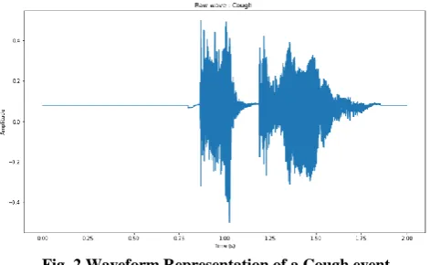
[image:2.595.308.544.354.499.2]

Audio representation of the waveform is not computationally expensive. It shows how the amplitude of samples varies over time. A waveform representation is used to find the beginning and end of audio events, notably how the samples are distributed across the time. Figure 2 shows an example of audio waveform. Generally, Speech / Audio are a non stationary signal. So it is important to convert a signal from time domain and frequency domain. During this process, Fast Fourier Transform (FFT) may produce distortions on high frequency.

Fig. 2 Waveform Representation of a Cough event

(3)

[image:3.595.85.521.60.192.2]

Fig. 3 Windowed sampled audio frame Generally audio recognition tasks are carried out with

feature extraction and learning process. Learning process is handled by the classifiers such as CNN, RNN etc. Signal processing techniques are used to perform feature extraction in any audio / speech signal based on the acoustic domain

[image:3.595.82.496.304.421.2]

knowledge [9]. In many previous works, existing audio features are rather associated by concatenating MFCC and other spectral features. These are choosen heuristically which may be redundant in most applications and insufficient based on the data.

Fig. 4 MFCC Extraction A variety of machine learning algorithms were developed

by machine learning community to discover and represent the audio features. This learning approach is commonly referred as feature learning or feature representation. Recently, Deep Neural Network (DNN), and CNN are widely used in speech / audio recognition.

In audio domain, learning from raw audio is mainly researched in automatic speech recognition [10]. Deep learning models are strong to classify the raw audio sounds. It turns out that extracting relevant features from audio signal is still useful. The extracted feature should be relevant to the

content of audio so that acoustic events can be recognized. In the proposed work MFCC and raw audio features were used. MFCC feature extraction is shown in Fig. 4.

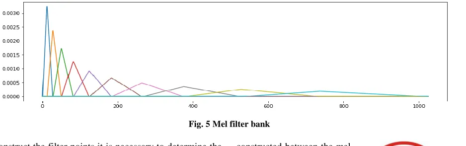
After preprocessing the mel filter banks coefficients are computed to the given audio frames, that provide more relative information about the power in each frequency band. The filter bank grows exponentially with frequency based on the space between the filters. The filter bank for any frequency band can be produced. Figure 5 shows the filter bank of an audio sample for the whole frequency band.

Fig. 5 Mel filter bank

To construct the filter points it is necessary to determine the start and stop of filters. Initially the filter bank edges are converted to the mel space and a linearly spaced array is

[image:3.595.67.536.604.751.2]

(4)

space and normalized it with the FFT array size. Mel filtered signal is passed through a logarithmic computation, and finally MFCC are computed by applying Discrete Cosine Transform (DCT).

IV. EXPERIMENTAL PARAMETERS

A. Datasets

The audio dataset used for the proposed work was released by Freesound which is annotated with labels based on Google Audioset Ontology. The audio file consists of 41 categories of 16-bit PCM, 44.1 kHz, and mono wav files of invariable length. Figure 6 illustrates the dataset distribution. The categories include ‘Acoustic guitar’, ‘Applause’, ‘Bark’, ‘Bass drum’, Burping or eructation’, ‘Bus’, ‘Cello’, ‘Chime’, ‘Clarinet’, ‘Computer keyboard’, ‘Cough’, ‘Cowbell’, ‘Double bass’, ‘Drawer open or close’, ‘Electric piano’, ‘Fart’, ‘Finger snapping’, ‘Fireworks’, ‘Flute’, ‘Glockenspiel’, ‘Gong’, ‘Gunshot or gunfire’, ‘Harmonica’, ‘Hi hat’, ‘Keys jangling’, ‘Knock’, ‘Laughter’, ‘Meow’, ‘Microwave oven’, ‘Oboe’, ‘Saxophone’, ‘Scissors’, ‘Shatter’, ‘Snare drum’, ‘Squeak’, ‘Tambourine’, ‘Tearing’, ‘Telephone’, ‘Trumpet’, ‘Violin or fiddle’, ‘Writing’.

Fig.6 Number of samples per category

The organization of the dataset includes 9.5k of train set and the same amount of test set. The train set is unequally distributed with a maximum of 300 samples per category and minimum of 94 samples. Out of 9.5k samples in train set, only 3.7k samples are manually verified annotations and 5.8k samples are unverified annotations. Hence the data provided is an imbalanced dataset whose performance is evaluated using Mean Average Precision.

B. Convolutional Neural Network (CNN)

Neural Networks is a machine learning technique which is modeled based on the structure of human brain. It consists of networks of learning units called neurons. A CNN is an artificial neural network composed of neurons with learning weight and bias. Each neuron receives several inputs, takes over a weighted sum of input and passes through activation function to generate an output [11]. CNNs are designed to process multiple arrays of data. It includes 1D for signals and sequences, 2D for images and audio spectrograms, and 3D for video data. CNN uses local links, weights, pooling and multilayer usage as the key properties from any signal. A typical CNN is organized as a number of stages.

C. Convolution layer

The first stage is composed of convolutional layers and pooling layers. Neurons are organized into feature maps in a Convolutional layer, in which each unit feature maps from previous layer is connected to local patches via set of weights. The result of this weighted sum value is then passed through a non linear activation function called ReLU. The function of convolution layer is to learn and detect low level features in previous layer, while the role of pooling layer is to merge those similar features into one context. The pooling layer takes input from patches which are shifted by several rows and columns, reduces the dimensions of representation and creates as invariance to small distortions in order to reduce the number of learning parameters.

D. Max pooling

It is the most popular way for pooling which extracts the maximum value in each patch and to discard all other values in a feature map.

E. Global Average pooling

A global average pooling down samples the feature map dimension into 1D arrays by using average of all elements on feature map. The advantages of using average pooling are reducing the number of learning parameters, and to accept the input of variable sizes.

F. Fully connected layer

The output features maps of last convolutional or pooling layer is flattened into 1D array and connected to one or more fully connected layers. After the features are extracted by convolutional layer, and down sampled by pooling layer, they are mapped to final outputs in network by a fully connected layer which performs classification. The convolution, non linearity, and pooling stages are repeated and stacked, followed by fully connected layers.

The kernel is the important parameter automatically learned during the training process in a CNN. The hyper parameter of a convolutional layer includes kernel size, number of kernels, strides, padding, and activation function. The pooling layer learns the hyper parameters like pooling method, filter size, strides, and padding. A fully connected layer learns the weights, number of weights, and activation function. Other hyper parameters required to fine tune the CNN includes optimizer, learning rate, loss function, mini batch size, epochs, regularization, and weight initialization. G. Learning rate

The learning rate is defined in order to optimize and minimize the loss function of a CNN model and controls how much the optimization algorithm needs to update its weights. Depending on the choice of the optimizer, the learning rate can be either fixed or varied. Different optimizers are available in CNN which includes Stochastic Gradient descent (SGD), Adam, Adagrad, AdaDelta or RMSProp. Usually the default learning rate works well with Adam optimizer.

H. Mini batch size

Batch size is a term used in machine learning which describes the number of samples included for training in single iteration. The standard batch sizes used are 8, 16, 32, or 64. If the batch size is selected too small, then gradient descent will not be smooth which will makes the model to learn slowly and there may

(5)

If the batch size is too high then it may take long time to train.

I. Dropout

Dropout is a regularization technique used to prevent over fitting of the deep learning model. This method is used to drop some range of units in neural network according to desired ratio. A fully connected layer takes most of parameters and therefore during training, the neurons acquire interdependency with each other which limits the power of each neuron may lead to over fitting of training data.

V. EXPERIMENTAL RESULTS AND DISCUSSION The signal must be preprocessed in advance and divided into successive windows and frames in order to extract relevant information from the audio signal. Initially pre emphasis filter is applied on a signal to amplify the high frequency. After pre emphasis we must divide the signal into short term frames. Librosa library is used to extract the MFCC coefficients with a 25ms for the frame size and 10ms stride on 50% overlap.

A baseline system is based on a CNN classifier which is scaled down from a deep CNN model. It allows training a

fully connected multi layer perceptron which is built on tensorflow. The baseline CNN model consists of three 2D convolutional layers with ReLU activation functions and 2D maxpool layers, followed by max reduction and softmax layer. Adam optimizer is used to train the model with a leasrning rate of 1e-4 with a batch size of 64. Conv2D with kernel size and strides are (7x7, 1), (5x5, 1) and (3x3, 1) correspondingly on each layers. Maxpool2D and Conv2D use the ‘SAME’ padding scheme. The baseline system performed with a Mean average precision of 0.7.

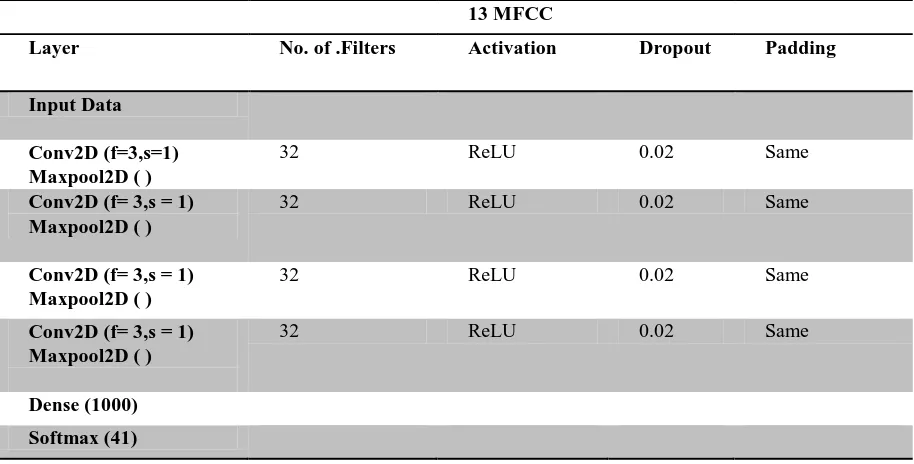
[image:5.595.70.527.359.591.2]

The proposed CNN model for audio tagging was developed on Google Colab. Colaboratory is a cloud service based on jupyter notebook for machine learning research which improves working with deep learning libraries like PyTorch, Keras, and TENSORFLOW. Colab supports Graphics Processing Units (GPU) as a backend for free. It is used as a tool for accelerating deep learning applications. The CNN architecture proposed consists of four 2-D Convolutional layers with 3x3 kernels, followed by 2-D max-pool layers with 3x3 filters. ‘ReLu’ activation is used in all layers with 0.02 dropout ratio. Table 1 illustrates the parameters used in proposed CNN architecture.

Table 1 Proposed CNN model -1

13 MFCC

Layer No. of .Filters Activation Dropout Padding

Input Data Conv2D (f=3,s=1) Maxpool2D ( )

32 ReLU 0.02 Same

Conv2D (f= 3,s = 1) Maxpool2D ( )

32 ReLU 0.02 Same

Dense (1000) Softmax (41)

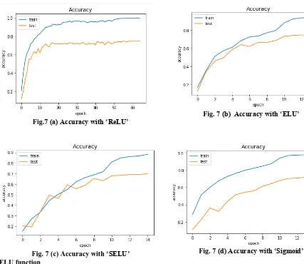
The Adam optimizer with a learning rate of 0.003 and a batch size of 128 samples is used. The model is trained initially with 10 epochs. Based on the performance the number of epochs is varied up to 50. The proposed model generalized with a novel data performed with an accuracy of 75% and the novel data was verified by undergoing audio visualization using python library. The proposed model has been tried with following activation functions in order to improve the performance of the network. The same parameter with sigmoid activation function in all convolutional layers is trained.

Sigmoid function

(6)

Fig.7 (a) Accuracy with ‘ReLU’

Fig. 7 (b) Accuracy with ‘ELU’

Fig. 7 (c) Accuracy with ‘SELU’ Fig. 7 (d) Accuracy with ‘Sigmoid’ ELU function

Exponential Linear Unit (ELU) is an activation function which has zero converge cost and produces better accuracy. ELU is similar to ReLU except negative inputs. Hence it can be used for higher classification models comparing to traditional ReLU. The advantage of using ELU is it makes the mean activation closer to zero which enhances the training speed of the model.

SELU function

Scaled Exponential Linear Unit (SELU) comes with an advantage over ReLU of dealing with internal normalization which handles vanishing gradients problem. ‘SELU’ learns on its own faster and better than other activation functions, while combined with batch normalization. Though there is no real difference with RELU, SELU outperforms more significantly. The accuracy obtained with different activation functions of proposed model is shown in Fig.7 (a) to (d). Among the different activations, ‘ReLu’ and ‘elu’ functions outperformed others.

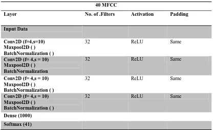
The proposed model with 13 MFCC coefficients does not improve the performance of audio tagging system. So the audio tagging model was trained with 40 MFCC coefficients with small variations in the proposed parameters. Table 2 illustrates the CNN architecture with varied parameters.

[image:6.595.48.475.46.416.2] [image:6.595.49.266.60.411.2]

(7)

[image:7.595.90.506.62.317.2]

Table 2 Proposed CNN Model -2 40 MFCC

Layer No. of .Filters Activation Padding

Input Data Conv2D (f=4,s=10) Maxpool2D ( )

BatchNormalization ( )

32 ReLU Same

Conv2D (f= 4,s = 10) Maxpool2D ( ) BatchNormalization

32 ReLU Same

Dense (1000) Softmax (41)

Batch Normalization

To speed up the learning, it is essential to normalize the input layer by adjusting and scaling the activations. Batch normalization generally reduces the covariance shift. The advantage of using batch normalization is it allows each network layer to learn something more independently of other layers by itself. It reduces the model getting into overfit because of regularization effects. Therefore, less dropout rate can be used to learn features. This parameter normalizes the output of a previous activation layer to increase the stability of a neural network by subtracting the batch mean and dividing it by the batch standard deviation.

This model outperformed with an accuracy of 92% as shown in Table 3. Once the model is trained, the prediction is performed with average mean precision with top 3 labels. The test data along with predicted labels are presented and visualized using Ipython.

Table 3 Predicted Label

S. No. FNAME LABEL

1 00063640.wav ‘Finger snapping’

‘Fireworks’ ‘Telephone’ 2 0013a1db.wav ‘Oboe’ ‘Flute’ ‘Clarinet’ 3 002bb878.wav ‘Bass drum’ ‘Snare drum’

‘Hi hat’ 4 002d392d.wav ‘Bass drum’ ‘Electric

piano’ ‘Hi hat’ 5 00326aa9.wav ‘Oboe’ ‘Flute’ ‘Clarinet’

6 0038a046.wav ‘Knock’ ‘Bass drum’

‘Bark’

7 003995fa.wav ‘Squeak’ ‘Violin or

fiddle’ ‘Telephone’

8 005ae625.wav ‘Acoustic guitar’

‘Saxophone’ ‘Gong’ 9 007759c4.wav ‘Acoustic guitar’ ‘Gong’

‘Clarinet’

The overall test classification report for the proposed second model is illustrated with the precision and recall metrics as shown in Table 4. The average precision and recall are calculated by using equations and , where true positives ( , false positives , true negatives ), and false negatives predicts the ground truth of entire evaluation data.

 Precision : The ability to return only relevant cases of a classification model.

 Recall : The ability to identify all relevant occurrences of a classification model.

 F1-score: A metric that uses harmonic means to combine recall and precision.

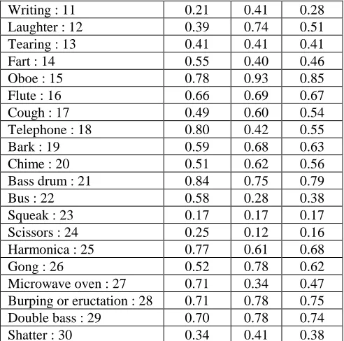
Table 4 Classification Report for Proposed CNN Model – 2

Categories Precision Recall f1-score

Hi hat : 0 0.72 0.54 0.62

Saxophone : 1 0.74 0.72 0.73

Trumpet : 2 0.72 0.70 0.71

Glockenspiel : 3 0.44 0.62 0.51

Cello : 4 0.84 0.69 0.76

Knock : 5 0.67 0.67 0.67

Gunshot or Gunfire : 6 0.81 0.27 0.40

Clarinet : 7 0.75 0.80 0.78

Computer keyboard : 8 0.67 0.15 0.25

Keys jangling : 9 0.50 0.50 0.50

(8)

Writing : 11 0.21 0.41 0.28

Laughter : 12 0.39 0.74 0.51

Tearing : 13 0.41 0.41 0.41

Fart : 14 0.55 0.40 0.46

Oboe : 15 0.78 0.93 0.85

Flute : 16 0.66 0.69 0.67

Cough : 17 0.49 0.60 0.54

Telephone : 18 0.80 0.42 0.55

Bark : 19 0.59 0.68 0.63

Chime : 20 0.51 0.62 0.56

Bass drum : 21 0.84 0.75 0.79

Bus : 22 0.58 0.28 0.38

Squeak : 23 0.17 0.17 0.17

Scissors : 24 0.25 0.12 0.16

Harmonica : 25 0.77 0.61 0.68

Gong : 26 0.52 0.78 0.62

Microwave oven : 27 0.71 0.34 0.47

Burping or eructation : 28 0.71 0.78 0.75

Double bass : 29 0.70 0.78 0.74

Shatter : 30 0.34 0.41 0.38

Fireworks : 31 0.19 0.53 0.28

Tambourine : 32 0.89 0.85 0.87

Cowbell : 33 0.73 0.83 0.78

Electric piano : 34 0.54 0.47 0.50

Meow : 35 0.64 0.48 0.55

Drawer open or close : 36 0.62 0.69 0.66

Applause : 37 0.82 1.00 0.90

Acoustic guitar : 38 0.51 0.51 0.51

Violin or fiddle : 39 0.96 0.69 0.80

Finger snapping : 40 0.74 0.70 0.72

[image:8.595.46.292.50.294.2]

Table 2 illustrates that among 41 categories of acoustic events, almost maximum event occurrences are predicted correctly based on the precision and recall values in the classification report. Few events like Hi hat, Cello, Computer Keyboard, Fart, Bass Drum, Bus, Scissors, Microwave oven, Meow, and Violin were found to be identified with fewer relevancies. Hence the proposed CNN model 2 performs better with previous model and the plot of precision and recall report is sown in Figure 8.

Fig. 8 Precision – Recall Plot

VI. CONCLUSION

The general purpose audio tagging system based on deep learning model can be effectively used in various audio based information retrievals. The large scale data used for analysis contains subsets of training data with imbalanced annotations of varying reliability and variable length of audio files. To handle the large scale data, Google Colab cloud service with GPU has been used which improved the learning speed of the models. A baseline system on CNN model is performed with a average mean precision of 0.7 with more than 12 hours of training. The proposed CNN models are discussed with different input representations using MFCC features resulted better performance comparing with a baseline with 92% of accuracy. The work is in progress to learn the features from raw wave using Apache Spark framework.

REFERENCES

1. Jongpil Lee and Juhan Nam, “Multi-Level and Multi-Scale Feature

Aggregation using Pre trained Convolutional Neural Networks for Music Auto-Tagging”, IEEE Signal Processing Letters, Vol.24, No. 8, Aug 2017.

2. Qiuqiang Kong, Yong Xu, Wenwu Wang, Mark D. Plumbley, “A Joint

Detection-Classification Model For Audio Tagging Of Weakly Labelled Data”, International Conference on Acoustics, Speech and Signal Processing (ICASSP), IEEE, 2017.

3. Yong Xu, Qiuqiang Kong, Qiang Huang, Wenwu Wang, and Mark D.

Plumbley, “Convolutional Gated Recurrent Neural Network Incorporating Spatial Features for Audio Tagging”, IEEE, 2017.

4. Turab Iqbal, Qiuqiang Kong, Mark D. Plumbley, Wenwu Wang,

“General-Purpose Audio Tagging from Noisy Labels using Convolutional Neural Networks” Detection and Classification of Acoustic Scenes and Events, 2018.

5. Matthias Dorfer, and Gerhard Widmer, “Training General-Purpose

[image:8.595.301.552.50.172.2]

(9)

6. Nam Kyum Kim, Jeong Hyeon Yang, Jeong Eun Lim, Jinson Park, Ji

Hyun Park, and Hong Kook Kim, “ Gist_Wisenetai Audio Tagger Based On Concatenated Residual Network For Dcase 2018 Challenge Task 2”, Detection and Classification of Acoustic Scenes and Events, 2018.

7. Qingkai WEI, Yanfang LIU, and Xiaohui RUAN, “A Report on Audio

Tagging with Deeper CNN, 1d-Convnet and 2d-Convnet”, Detection and Classification of Acoustic Scenes and Events, 2018.

8. Marcel Lederle and Benjamin Wilhelm, “Combining High-Level

Features of Raw Audio and Spectrograms for Audio Tagging”, Detection and Classification of Acoustic Scenes and Events, 2018.

9. Juhan Nam, Jorge Herrera, and Kyogu Lee, “A Deep Bag-of-Features

Model for Music Auto-Tagging”, CoRR, 2015.

10. Jongpil Lee Jiyoung Park Keunhyoung Luke Kim Juhan Nam,

“Sample-Level Deep Convolutional Neural Networks for Music Auto-Tagging using raw waveforms”, 14th Sound & Music Computing Conference, 2017.

11. Yann LeCun, Yoshua Bengio, and Geoffrey Hinton, “Deep Learning”,

Nature, 2015.

AUTHORS PROFILE

Ms. E. Sophiya earned her bachelor's degree in Computer Science and Engineering from Ponnaiyah Ramajayam College of Engineering and Technology. She received her master’s degree in Computer Science and Engineering from Annamalai University. She has working experience as Assistant Professor in Christ college of Engineering and Technology, Puducherry. She is currently pursuing PhD (Full Time) in Computer Science and Engineering at Annamalai University. Her research is focused on Audio Scene Classification, Event Detection, Large scale data,Machine learning, and deep learning.

Dr. S. Jothilakshmi earned her bachelor's degree in electronics and communication engineering from Madras University. She received doctoral and master's degrees in computer science and engineering from Annamalai University. She was a postdoctoral researcher at Marshall University, United States of America. She currently works as

Associate professor in Department of