International Journal of Innovative Technology and Exploring Engineering (IJITEE) ISSN: 2278-3075, Volume-9 Issue-2, December 2019
Abstract:
In the brain tumor MRI images, the identification, segmentation and detection of the infectious area is a tedious and lengthy task. As segmentation is called intensity inhomogeneity by an intrinsic object. In this paper we suggest an energy efficient minimization technique for joint domain assessment and segmentation of MR images called multiplicative intrinsic component optimization (MICO). In this work, we focused on quicker implementation with a robust removal of gray-level co-occurrence matrix (GLCM). Optimal texture characteristics are obtained by the Spatial Gray Dependence (SGLDM) technique from ordinary and tumor areas. With very large feature sets, the choice of features is redundant because the precision frequently worsens without choice of features. However, when only the feature selection is used, the precision of classification is significantly improved. However, by reducing the time needed for classification computations and improving classification precision by removing redundant, false or incorrect characteristics. A fresh function choice and weighting technique, supported by the decomposition developmental multi-objective algorithm, are provided in this work. These characteristics are provided for the MPNN classification. Modified probabilistic neural network (MPNN) classification was used in brain MRI images for training and testing for precision in tumor identification. The simulation findings accomplished almost 98% precision in the identification of ordinary and abnormal tissue from brain MR images showing the efficiency of the method suggested.
Index Terms: Brain segmentation, Intensity inhomogeneity, Texture features, Probabilistic Neural Networks, Bias field estimation
I. INTRODUCTION
The vision of the unusual constructions of the human brain with easy imaging methods is very hard. The method of magnetic resonance imaging separates and clarifies human brain neural architecture. The MRI method includes many processing methods which scan the inner framework of the human brain and seize it. Tumor malignant Grade III and Grade IV are increasing rapidly and can affect healthy brain cells and spread to other areas of the brain or spinal cord. Detection, identifying and classification of such brain tumors
Revised Manuscript Received on December 05, 2019.
Bobbala Sreedevi, Research Scholar in JNTUH and Working as Assistant Professor, Dept. of ECE, Vaagdevi College of Engineering, Warangal Telangana, India.
Dr.T.Anil Kumar, Professor, Department of ECE, CMR Institute of Technology, Hyderabad, Telangana, India.
Dr. K. Kishan Rao , Professor, Department of ECE, Sreenidhi Institute of Science and Technology, Hyderabad, Telangana, India.
in previous stages is thus a severe problem in medical research. Due to bad radio wave coil uniformity and gradient-driven Eddy currents in the brain magnetic resonance (MR), the segmentation precision is seriously affected by sound and intensity inhomogeneity (preference). In reality, however, brain MR image has certain shortcomings, such as sound intrusion, inhomogeneity of intensity, poor contrast and the brain tissue's total size impact. It is therefore very hard to precisely segment brain MR images. Most techniques now suppose that the allocation of intensity in MR images is uniform only from the viewpoint of anti-noise output to a MR section, which is bound to result in incorrect segmentation.
To obtain greater segmentation precision, the bias field of MR images must be estimated. It sees only pixel-relevant data in the image while forgetting the impact of the noise sensitive neighborhood spatial pixels. The human prediction is not always correct [4]-[8], it's sometimes wrong, but the computer can't. Automated classification and identification of the tumors indifferent medical images are simulated by the inevitable elevated precision of a user’s existence. Many scientists have therefore proposed a sequence of enhanced algorithms [4–9]. PNN is a data classifier suggested by authors in [1] and [2] Probabilistic neural network. It draws scientists in the sector of machine learning. PNN applications can be primarily found in medical treatment and forecast in literature [3]. An efficient technique is suggested for extracting characteristics from MR images with reduced computing needs and classification outcomes are evaluated. The main contributions and organization of this paper are summarized as follows: In section 2 we describe related works of several authors’ works toward classification of brain tumors methods. The section 3 methods and methodology of proposed work. The section 4 deliberates results and discussions. Finally in section 5 we concluded the paper.
II. BACKGROUNDWORKS
Intensity inhomogeneity are frequently presumed to be assigned to a spatially variable domain, which is a multiplicative component of the measured image. This multiplicative component, referred to as the bias field, differs in space due to inhomogeneity of the areas B0 and B1.
An Efficient
Method
for Automatic
Classification of Brain MRI using Feature
Selection
and Modified Probabilistic Neural
Network
Probabilistic Neural Network
Bias field adjustment means a process to assess the imagebias field to eliminate its impact. In [9], the authors suggested an Automated Segmentation and Classification MR approach whereby an SVM classification was used for the matrix of ordinary and unusual images with statistical characteristics. In [10], the authors noted that the classification frequency for a SVM classification system is greater than the self-organized map strategy of neural networks. SVMs will demonstrate their superior efficiency and feasibility in the ranking of brain cells in classical techniques of highest probability. The authors used the EM algorithms to detect anomalies in [11]. These algorithms demonstrated to distinguish big tumors from the brain cells surrounding them by training them solely on ordinary brain images to acknowledge a departure from normality in healthy individuals. This needs a strong level of computer effort. The knowledge-based methods made the segmentation and classification findings more effective, but these methods needed extensive practice. Although a significant amount of level set techniques [12-14] have been widely investigated to tackle the strength of homogenization, few [15-16] take into consideration the intensity inhomogeneity estimate.
III. METHODSANDMETHODOLOGY In this paper we designed efficient framework for all the stages of MRI grade classification at different stages and their functionalities.
A. Data Acquisition
The data set required for simulation assessment is acquired from multiple clinics in India and only a few from different websites. The database comprises of 50 MR images, out of which 30 are cancer images and the other 20 are normal. The patient's age in the database is between 30 and 60 years. Each image has a resolution of 512x 512 with DICOM format. The dataset comprises of multi-spectral MRI scans (T1, T2, FLAIR).
B. Modified pre-processing:
Medical image assessment needs preprocessing, because imaging tools may add noise to MR images. Bias field correction itself is a significant job in the production of medical images. We suggest a fresh method to bias field measurement and tissue segmentation in an energy minimization structure in this work.
Decomposition of MR images into multiplicative intrinsic components:
From the formation of MR images, it has been generally accepted that an MR image I can be modeled as
I x
b x J x
n x
(1)where I(x) is the intensity of the observed image at voxel x, J(x) is the true image, b(x) is the bias field that accounts for the intensity inhomogeneity in the observed image, and n(x) is additive noise with zero-mean. The bias field b is assumed to be smoothly varying. The true image J characterizes a physical property of the tissues being imaged, which ideally take a specific value for the voxels within the same type of tissue.
Fig.1. Overall process of MRI classification
In this paper, we consider (1) as a decomposition of the MR image I into two multiplicative components b and J and additive zero-mean noise n. In this paper, we propose a method that uses the basic properties of the true image and bias field, namely, the piecewise constant property of the true image J and the smoothly varying property of the bias field b. The decomposition of the MR image I into two multiplicative intrinsic components b and J with their respective spatial properties.
Energy formulation for multiplicative intrinsic component optimization
We put forward an energy minimization formulation for bias field estimation and tissue segmentation based on the image model (1) and the intrinsic properties of the bias field and the true image. In view of the image models (1), we consider the problem of finding the multiplicative intrinsic components b and J of an observed MR image I such that the following energy is minimized.
2Ω
, | |
F b J
I x b x J x dx(2)
With these representations of the true image J and bias field b, the energy F(b, J) can be expressed in terms of three variables, u = (u1, ⋯, uN)T, c = (c1, ⋯, cN)T, and w = (w1, ⋯, wM)T, namely,
21 Ω
( ,
, ,
|
|
N T
i i i
F b J
F
I x
G x
c u x
dx
u c w
w
(3)
Thus, the optimization of b and J can be achieved by minimizing the energy F with respect to u, c, and w.
C. Feature extraction:
Features of an image are the characteristics that define the image entirely. The issue with the absence of efficient selection strategies in most
International Journal of Innovative Technology and Exploring Engineering (IJITEE) ISSN: 2278-3075, Volume-9 Issue-2, December 2019
The gray level co-occurrence matrix (GLCM) is the basis for our removal function based on Haralick et al. Method. Method. This statistical technique calculates each image’s co-occurrence matrix in the database, by calculating how many times a pixel with a certain intensity I occur with a reference to a certain range d and position j of a pixel. The matrix is calculated for only one path (θ =0) and one range (d=1) in this document. The gray level matrix shows certain characteristics that affect the temporal allocation of the Gray concentrations in an image item.
D. Feature Selection:
The task of feature selection (FS) is to remove the features and only select features sufficient to resolve a problem, thus reducing the overhead and improving classification accuracy.
Feature Selection and Weighting:
Suitable classification of data points requires that the data points of distinct groups are usually distinct and that those of the same category are as close as necessary to each other. The dimensions of such inter-class separability and intra-class proximity depend on the characteristics of the data points. Therefore the objective of the proposed feature selection algorithm is two-fold: to both select features and to weigh them in order to simultaneously optimize the intra-class distance and the inter-class distance of the resulting data points.
Multi-objective Optimization:
[image:3.595.314.547.373.636.2]An MOP involves the development of numerous (generally conflicting) objective features with or without restrictions. Generally, these objective function conflict, i.e. the adjustment of one objective function to its desired value will result in a deviation from the ideal value of another objective function.
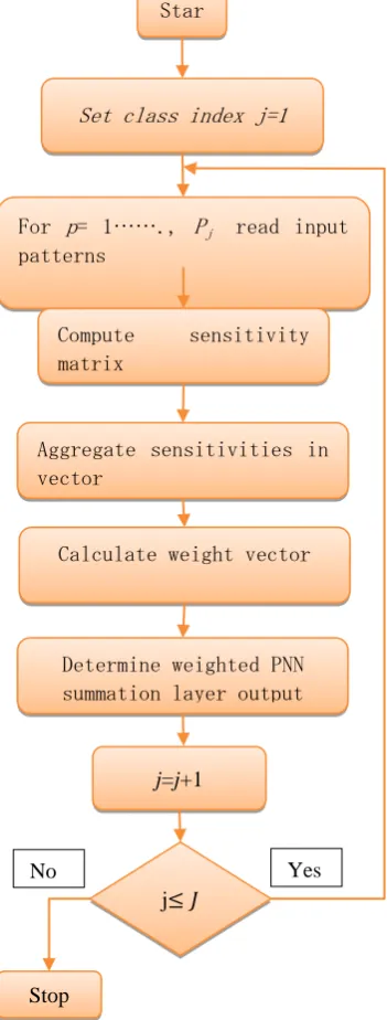
Fig. 2. Flow chart of Multi-objective Optimization process
The comparison of candidate solutions has been achieved by the concept of Pareto-optimality, where a better balance is acquired between these objectives features, thereby recovering several solutions after optimization, recognized as the ideal Pareto set. Then one option is selected from the ideal front of Pareto, based on the implementation. Only those
features chosen forms the new subset of features after the corresponding weights have been applied to them. In this sub-set of weighted characteristics, any classification algorithm may be implemented. The following flow graph is given for the full algorithm.
Classification using modified Probabilistic neural network (MPNN):
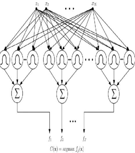
It comes from the Bayesian network and statistical algorithm called the discrimination assessment of Kernel Fisher. It consists of 4 layers and nodes: input layer, hidden layer, pattern layer and output layer. In the shape of a neural network, PNN formulates weighted neighbors. The input layer is ' P ' neuron which depends on categorical factors of different functionalities obtained with a gray-level co-occurrence matrix (GLCM). The weights of the input node were held 1, which were transmitted into a hidden layer. Radial base features have been calculated in the pattern layer and are introduced into the summation layer. The summary layer provides the weighted activation values in each hidden layer category. The summation layer values have been supplied into the output layer. The input layer selects the largest probability, 1 for the target class form shows positive and 0 for the non-targeted class form suggests negative. This network's training scheme consists of the suitable selection of the smoothing parameter hi using the plugin technique and the calculation of the change ratio Sp. Figure.3 shows the framework of the PNN system.
Fig. 3. The architecture of probabilistic neural network.
[image:3.595.65.254.498.684.2]Probabilistic Neural Network
Fig.4. The algorithm for the computation of the weights in PNN between pattern and summation layer
In Fig. 4, we present the step-by-step data classification algorithm with the use of modified PNN model. We start with the calculation of the sensitivity coefficients for all r = 1, 2, . . . , Pj neurons in the pattern layer.
IV. RESULTSANDDISCUSSION
Our method was extensively tested on synthetic and true MRI information during the modified preprocessing stage, including 1.5T and 3T MRI data. In this section, we first demonstrate simulation outcomes for certain synthesized and true MR images, including certain images with serious intensity inhomogeneities.
Fig.5. Results for images with severe intensity inhomogeneity presented in the first column. The estimated bias fields, segmentation outcomes, and bias
field corrected images are shown in columns 2, 3, 4, correspondingly
For the image in the first row of Fig. 5, we used MICO to create a systematic attempt to tackle the serious inhomogeneities of our method. The computed bias field, outcomes and the brain area adjusted images acquired from our method are shown in the second, fifth and fourth rows respectively. Whereas the images are highly intensive, our method can produce desirable results of field correction and segmentation of tissues as illustrated in Fig.5.
Table 1. Comparison of NSGA-II and Our method
Dataset NSGA-2 Our method
Accuracy (No.of features)
Time (s) Accuracy (No.of features)
Time (s)
Iris 96.03(2) 05.08 96.03(2) 1.56
Heart 78.89(12) 05.19 78.89(5) 1.79
Brain tumor
97.23(9) 04.31 97.23(7) 02.12
Because of its shorter time and a better choice of our non-dominant alternatives as illustrated in Table 1. The same target set as the present method is used for contrast with NSGA-II, a well-known multi-target optimizer. The quantity of features selected chosen and the time our approach takes significantly less than NSGA-II. Both techniques have been performed in the scheme under comparable conditions.
Star t
Set class index j=1
For p= 1……., Pj read input
patterns
Compute sensitivity
matrix
Aggregate sensitivities in vector
Calculate weight vector
Determine weighted PNN summation layer output
j=j+1
j≤ 𝐽
Stop
[image:4.595.91.267.72.535.2]International Journal of Innovative Technology and Exploring Engineering (IJITEE) ISSN: 2278-3075, Volume-9 Issue-2, December 2019
[image:5.595.306.549.51.215.2]Fig.6. performance of GLCM features 1 and 2 From Fig. 6, it is shown that execution time for 10 GLCMs inputs are approximately 40sec and CPU time is around 35sec.
Fig.7. performance of GLCM features 3 and 4 From Fig. 7, it is shown that execution time for 10 GLCMs inputs are approximately 0.5sec and CPU time is around 0.8 sec. So GLCM feature 3 and 4 outperforms as related to GLCM feature 1 and 2.
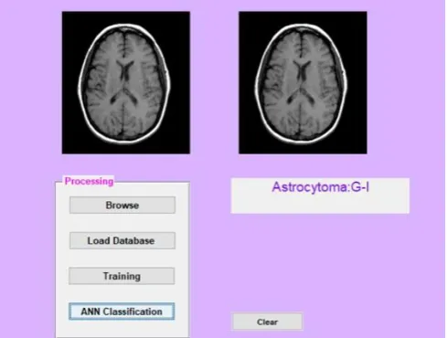
Fig.8
.
Grade classification of image1Fig. 9
.
Grade classification of image 2Fig.10
.
Grade classification of image 3Fig.11
.
Grade classification of image 4 V. CONCLUSION [image:5.595.304.550.247.411.2] [image:5.595.48.292.296.488.2] [image:5.595.304.550.443.592.2] [image:5.595.47.292.559.744.2]Probabilistic Neural Network
REFERENCES1. D. F. Specht, “Probabilistic neural networks,” Neural Networks, vol. 3, no. 1, pp. 109–118, 1990.
2. “Probabilistic neural networks and the polynomial adaline as complementary techniques for classification,” Neural Networks, IEEE Transactions on, vol. 1, no. 1, pp. 111–121, Mar 1990. DOI: 10.1109/72.8021008.
3. R. Folland, E. Hines, R. Dutta, P. Boilot, and D. Morgan, “Comparison of neural network predictors in the classification of tracheal–bronchial breath sounds by respiratory auscultation,” Artificial intelligence in medicine, vol. 31, no. 3, pp. 211–220, 2004.
4. Issac H. Bankman, Hand Book of Medical Image processing and Analysis, Academic Press, 2009.
5. Sarah Parisot, Hugues Duffau, sr ephane Chemouny, Nikos Paragios, “Graph-based Detection, Segmentation & Characterization of Brain Tumors", 978-1-4673-1228-8 /12/2012 IEEE.
6. Neil M. Borden, MD, Scott E. Forseen, MD, "Pattern Recognition Neuroradiology", Cambridge University Press, New York, 2011.
7. Noramalina Abdullah, Umi Kalthum Ngah, Shalihatun Azlin Aziz, "Image Classification of Brain MRI Using Support Vector Machine", 978-1-61284-896-9/11/2011 IEEE.
8. Neuroradiology", Cambridge University Press, New York, 2011.
9. Antonie L., Automated Segmentation and Classification of Brain Magnetic Resonance Imaging, C615 Project, 2008, http://en.scientificcommons.org/42455248.
10. Chaplot S., Patnaik L.M., Jagannathan N.R., Classification of magnetic resonance brain images using wavelets as input to support vector machine and neural network, Biomedical Signal Processing and Control, 2006, 1(1), p. 86-92.
11.Gering D.T., Eric W., Grimson L., Kikins R., Recognizing deviations from normalcy for brain tumor segmentation, Lecture Notes in Computer Science, 2002, 2488, p. 388-395.
12.B.N. Shah J.K. Bhalani, Statistically Inhomogeneity Correction and Image Segmentation using Active Contours, Indian Journal of Science and Technology, 8 (1) (2017).
13. D.Y. Li, W.F. Li, Q.M. Liao, Active contours driven by local and global probability distributions, Journal of Visual Communication and Image Representation, 24 (5) (2013) 522-533.
14.C. J. He, Y. Wang, Q. Chen, "Active contours driven by weighted region-scalable fitting energy based on local entropy," Signal Processing, 92 (2) (2012) 587-600.
15. C.M. Li, C.Y. Kao, J.C. Gore, Z.H. Ding, Minimization of region-scalable fitting energy for image segmentation, IEEE Transactions on Image Processing, 17 (10) (2008) 1940-1949. 16. K.Y. Ding, L.F. Xiao, G.R. Weng, Active contours driven by