S C A L E A N D A B S T R A C T I O N : T H E S E N S I T I V I T Y O F F I R E - R E G I M E S I M U L A T I O N T O N U I S A N C E P A R A M E T E R S
I A N D A V I D D A V I E S
D E C L A R A T I O N
This thesis contains no material which has been accepted for the award of any other degree or diploma in any university. To the best of the author's knowledge, it contains no material previously published or written by another person, except where due reference is made in the text.
Canberra, September 2014
A B S T R A C T
Fire plays a key role in ecosystem dynamics and its impact on envir-onmental, social and economic assets is increasingly a critical area of research. Fire regime simulation models are one of many approaches that provide insights into the relative importance of factors driving the dynamics of fire-vegetation systems. The components of these sys-tems: climate, weather, terrain and ignition, mediated through veget-ation, operate over vast temporal and spatial scales when compared to that of human observation. Simulation provides a valuable way in which systems operating over these scales can be investigated, where analytical solutions may be intractable, data scarce or unavailable or field experiments prohibitively expensive or otherwise impractical.
Fire propagates as a contagious process and simulation offers an approach to capture this important behaviour explicitly. The patterns of fire regimes that emerge from such models are simply the sum of many fire events over time, each shaped by the changing weather, terrain and vegetation influencing the spreading fire. However, when formulating these models, space and time must be made discrete, and this entails introducing 'nuisance parameters': parameters necessary for the model formulation but not otherwise of interest. The most ob-vious of these are time step and spatial resolution. However, when points are traversed by fire during a simulation, how they are connec-ted (number of neighbours) and their arrangement (the distance and angle to each neighbour) can also be considered as nuisance paramet-ers required to describe a discrete geometry
Thus fire growth simulations are discrete approximations of con-tinuous non-linear systems, and it might be expected that the values chosen for these nuisance parameters will be important. While it is well known that discrete geometries have consequences for the shape and area of simulated fires, to my knowledge, no research has invest-igated the consequence this may have for estimates of the relative im-portance of the various drivers of fire regimes, which is after all, the key application of these models. Identifying the significance of spatio-temporal resolution and spatial representation has implications for model performance, the scales to which they can be realistically ap-plied and our confidence in their findings.
outcomes. A qualitatively different outcome would be, for example, that climate is found to be the most important determinant of fire re-gimes with one set of nuisance parameters but fuel management the most important with some other set.
Models are commonly either re-parameterised to account for changes in resolution or scaling-up methods applied if such exist. I will further argue that such differences as there are in model outputs due to spa-tial resolution, cannot be accounted for by either re-parameterising or using an approach that allows resolution to vary over the spatial extent as has been done in other fields.
A set of experiments were devised using a published fire regime simulation model, that I modified, verified and validated, to isolate just those aspects of the model's sensitivity to resolution and discrete geometries that are unavoidable or intrinsic to these choices. This new model (FIREMESH) is used to test the above hypotheses, using published experimental treatments that can stand as yardsticks by which formal estimates of the importance of nuisance parameters can be made.
As estimated by the model, neither spatio-temporal resolution nor any of the various choices available for discrete geometries, altered the model predichons with one exception: the use of spatial models that have only four neighbours between locations. This adds consider-able confidence to the robustness of this type of model. This finding holds for measures of the amount of fire in the landscape (average inter-fire interval), arguably, the major component of fire regimes. As expected, it is spatial resolution that has the greatest impact on run-ning times for the model but this study finds that neither calibration, nor taking an approach that allows resolution to vary over the spatial extent, can account for differences in model outputs that arise from running simulations at coarser resolutions.
A C K N O W L E D G M E N T S
This study has been undertaken at the Fenner School of Environment and Society, Australian National University with financial support from an Australian Postgraduate Research Award and a CSIRO Flag-ship PhD ScholarFlag-ship. I have many people to thank for their assist-ance during my research. In particular I would like to thank my su-pervisor Geoff Gary for encouragement, challenging ideas and new perspectives, not only during this study but over the course of many years. He has always been available for discussion and always with good grace and humour. I also owe a great debt of gratitude to Mal-colm Gill, someone who has experienced the development of fire sci-ence first hand in both Australia and around the world, and who has been generous with his time in providing guidance, always accom-panied by insight and precision. Both Geoff Gary and Malcolm Gill have provided stimulating discussion on many facets of the impact of fire on the environment and society both before and during this study.
Of particular value has been the opportunity to take part in an intentional model comparison study with researchers from Australia, North America and France. This has been a stimulating group whose ideas have in many ways led to this study I thank members of that group. Bob Keane, Russ Parsons, Mike Flannigan and Geoff Gary for the opportunity to present my initial ideas at a joint workshop at the start of this study in 2012.
I thank all members of my panel, Geoff Gary, Malcolm Gill, Steve Roxburgh and Jacques Gignoux for their detailed review of the draft of this thesis and for joint discussions over the course of the project. This work has benefited greatly from their insights and I have learnt much of what is required to undertake original research from these discussions. Of course, any errors and omissions remain my own.
I am grateful to Phil Zylstra for fire map data of the Australian Alps and for discussions of related work. Thanks also go to John Stein for his expertise in preparing terrain data on which this study is based, to Luciana Porfirio and Brendan Mackey for access to Landform 7 data and to Glem Davis for discussions on weather and climate data for SE Australia. I also would like to thank Bob Forrester for statistical ad-vice during this study, Joel Kelso for correspondence on fire spread on irregular grids and Lachie McGaw for discussions and data compar-ing rates of fire spread from Project Vesta and McArthur's Forest Fire Danger Meter. Geoff Gary has also been generous in providing both source code and data from the original version of FIRESGAPE (from some 16 years past) together with data from more recent studies with
which to validate the model used in this study. I also thank Professor Michael Barnsley for enthusiastic and animated discussions on fractal landscapes and look forward to continuing these discussions in the future.
C O N T E N T S
1 H Y P O T H E S E S A N D KEY C O N C E P T S 1 1.1 Introduction and hypothesis i 1.2 Fire models 4
1.2.1 Current research interest 4
1.2.2 Scales at which fire growth models are applied
1.2.3 Important applications of fire growth models 6 1.3 The fire regime concept 7
1.3.1 Intensity 8 1.3.2 Frequency 10 1.3.3 Seasonahty 1 1 1.3.4 Type 1 1
1.3.5 Spatial considerations 12 1.4 Systems and models as abstractions 13
1.4.1 Grounded abstractions 14 1.4.2 Scale 16
1.4.3 Physical-biological duality 17 1.4.4 Landscapes 18
1.4.5 Spatial representation: Models of space 18 1.5 Approach of this study 21
2 DATA R E Q U I R E M E N T S : T E R R A I N , V E G E T A T I O N , W E A T H E R A N D R E P L I C A T I O N 2 5
2.1 Overview of the model's data requirements 25 2.2 Terrain and vegetation 26
2.3 Climate 29
2.3.1 Extrapolating to other elevations 34 2.4 Replication of input data 36
2.4.1 Stochastic weather replication 36 2.4.2 Stochastic terrain replication 37
2.5 Matching available data to model requirements 42 2.6 Concluding remarks 43
3 F I R E M E S H : I T S O R I G I N S I N F I R E S C A P E A N D S U B S E Q U E N T M O D I F I C A T I O N S 4 5
3.1 Overview 45 3.2 Model 45
3.2.1 Model assumptions 46 3.2.2 Weather data 47 3.2.3 Models of space 48 3.2.4 Models of time 48
3.2.5 Projecting one-dimensional fire models to two dimensions 50
C O N T E N T S
3.2.8 Implementation in FIRESCAPE 58 3.2.9 Project Vesta 62
3.2.10 Implementation in FIREMESH 62 3.3 Concluding remarks 65
4 E X A M I N I N G T H E O P T I M A L U S E OF T E M P O R A L A N D S P A -T I A L D A -T A 6 9
4.1 Temporal and spatial resolution 69 4.1.1 Temporal resolution 70 4.1.2 Spatial resolution 74 4.1.3 Summary of findings 77 4.2 Mesh creation 77
4.2.1 Definition of equivalent spatial resolutions 77 4.2.2 Regular meshes 77
4.2.3 Triangulated Irregular Networks (TIN) 79 4.2.4 Generating even and uneven density
Triangu-lated Irregular Networks 81 4.3 Concluding remarks 89
5 M O D E L V E R I F I C A T I O N 9 I 5.1 Introduction 91
5.2 Consistency across resolutions using regular mesh con-figurations 92
5.3 Consistency across spatial resolution using triangulated irregular networks 93
5.4 Measuring area 101 5.5 Wind direction 108
5.6 Comparison of methods in deriving fire shape on Tri-angular Irregular Networks 1 1 1
5.7 Wind and slope interactions 114 5.8 Wind, slope, elevation and fuel 1 1 7 5.9 Terrain projection 121
5.10 Fuel change with time since last fire 122 5.11 Summary of findings 125
6 M O D E L A N D D A T A V A L I D A T I O N I 2 7 6.1 Introduction 127
6.2 Validation 130
6.2.1 Synthetic and Observed data 130
6.2.2 Simulation time required for stability of model outputs 131
6.2.3 Broad measures of comparison with FIRESCAPE 132 6.2.4 Ignition Neighbourhoods: Model skill in
real-ized niche generation 140 6.3 Replication of published experiments 142
6.3.1 Sensitivity to variation in terrain, fuel pattern, climate and weather 143
C O N T E N T S
6.4 Summary of findings 167
7 R E L A T I V E I M P O R T A N C E OF S P A T I O T E M P O R A L R E S O L U -T I O N 1 6 9
7.1 Introduction 169
7.2 Factors common to all experiments 169 7.3 Data analyis 172
7.4 Testing spatial and temporal resolution 175 7.4.1 Methods 175
7.4.2 Results 176 7.4.3 Discussion 180 7.4.4 Calibration 192
7.5 Summary of findings for spatio-temproal resolution 193 8 S P A T I A L R E P R E S E N T A T I O N : E X A M I N I N G D I F F E R E N T F O R M S
OF D I S C R E T E S P A C E I 9 7
8.1 Hypothesis (ii): Relative importance of neighbourhood number 198
8.1.1 Purpose 198 8.1.2 Methods 198 8.1.3 Results 198 8.1.4 Discussion 203
8.2 Hypothesis (iii): Importance of regular/irregular spa-tial representation 208
8.2.1 Purpose 208 8.2.2 Methods 208 8.2.3 Results 208 8.2.4 Discussion 213
8.3 Hypothesis (iv): Optimal sampling of space using a prior adapted mesh 216
8.3.1 Purpose 216 8.3.2 Method 216 8.3.3 Results 217 8.3.4 Discussion 221
8.4 Summary of findings for spatial representation 223 9 S Y N T H E S I S A N D F U T U R E D I R E C T I O N S 2 2 7
9.1 Synthesis 227
9.2 Generality of findings 231 9.3 Future directions 233
R E F E R E N C E S 2 3 7
A F I R E M E S H : O V E R V I E W , D E S I G N C O N C E P T S A N D D E T A I L S 2 5 9 A.I Purpose 259
A.2 Entities, state variables, and scales 259 A.3 Process overview and scheduling 261 A.4 Design concepts 262
C O N T E N T S
L I S T O F F I G U R E S
Figure i . i Level of interest in simulation modelling 5 Figure 1.2 Consequences of interpolating wind vectors 15 Figure 1.3 Graphic depicting a nested hierarchy of
ecolo-gical entities 17
Figure 1.4 Neighbourhood number density distribution for Delaunay triangulations 20
Figure 1.5 Regular and variable distribution of vertices in a discrete landscape 21
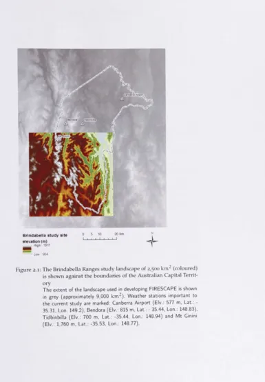
Figure 2.1 Study location 27
Figure 2.2 Observed fire size distribution 28 Figure 2.3 Density distributions of elevation, slope and
as-pect for the study site 29
Figure 2.4 Map of fuel steady state values 30 Figure 2.5 Monthly weather data (Canberra Airport
1985-2011) 31
Figure 2.6 Relative proportion of wind and modelled fire runs 32
Figure 2.7 Yearly weather data (Canberra Airport 1985-2011) 33
Figure 2.8 Empirically derived temperature lapse rates 35 Figure 2.9 Multi-scale standard deviations in elevation for
the Brindabella digital elevation model 39 Figure 2.10 Brindabella Ranges and derived fractal
land-scape 40
Figure 2.11 Comparison of aspects between real and fractal landscapes 41
Figure 3.1 Simulated fire burning on five different mesh configurations 49
Figure 3.2 Time / space diagram 51
Figure 3.3 Simple elliptical fire growth model 54 Figure 3.4 Ellipse metrics 54
Figure 3.5 Emprical length-to-breadth ratio functions 56 Figure 3.6 Back-fire rate of spread 57
Figure 3.7 Ellipse parameters required to shift the point from which the fire is assumed to propagate 58 Figure 3.8 Ellipse areas arising from three methods of
cal-culating the back-fire rate of spread 60 Figure 3.9 Three examples of fire shapes for 9 wind speeds
using FFDM 61
xiv List of Figures
Figure 3.11 Three examples of fire shapes for 9 wind speeds using modified FFDM 64
Figure 3.12 Isochrones showing the updated position of the fire front at half-hourly intervals 65 Figure 3.13 Polygons outlining burnt areas 66 Figure 3.14 Three magnifications of the same simulated fire
showing the heterogeneity of conditions over the course of the fire 66
Figure 3.15 Simulated fires burning at two different time steps 67
Figure 3.16 A simulated fire spreading over a Delaunay mesh triangulation with an irregular displace-ment of vertices 67
Figure 4.1 Changes in head-fire rate of spread at three dif-ferent time steps on two days of contrasting fire danger 71
Figure 4.2 Cumulative area burnt for time steps of 0.5 and 3 hours for two periods of contrasting fire danger 72
Figure 4.3 Differences in the vector sum of fire spread 73 Figure 4.4 A short transect of the study area showing the
rate of spread at each location determined by spatial components of fire spread 75 Figure 4.5 A transect of the study area showing Rn for
each location for a fire moving from left to right 76
Figure 4.6 Taxicab geometric system 78
Figure 4.7 Mesh minimum energy produced using the Capacity-Constrained Delaunay Triangulation 82 Figure 4.8 Sequence of steps in converting a digital image
into a Delaunay triangulation 84 Figure 4.9 Four surfaces depicting the steps involved in
creating a surface of the rate of change in the rate of spread of a head fire 85 Figure 4.10 A Delaunay triangulation using the
Capacity-Constrained Delaunay TriangulaHon algorithm 86 Figure 4.11 A Voronoi tessellation 87
Figure 4.12 Density distribution of ARh/AS 88 Figure 4.13 Density distribution of angles between
neigh-bouring vertices 89
Figure 5.1 Four, six and eight neighbour meshes at three hour time steps 95
List of Figures
Figure 5.3 Simulated and expected fire perimeter of a 24 hour fire 96
Figure 5.4 Simulated and expected fire perimeters on even Triangular Irregular Network meshes 97 Figure 5.5 Simulated and expected fire perimeters uneven
Triangular Irregular Network meshes 98 Figure 5.6 Mean and standard deviation of the radii of 10
replicate simulations with an even distribution of vertices 99
Figure 5.7 Mean and standard deviation of the radii of 10 replicate simulations with uneven distribution of vertices 100
Figure 5.8 Inherent error arising if area is calculated us-ing mesh length traversed 102
Figure 5.9 Complex polygon surrounding the fire perimeter of an 8 neighbour mesh 103
Figure 5.10 A tessellation of space using a combination of octagons and squares 103
Figure 5.11 Comparison of simulated and expected fire area at four spatial resolutions 105
Figure 5.12 Polygons placed around the perimeter of circu-lar fires on 4, 6 and 8 neighbour meshes 106 Figure 5.13 Comparison of two methods of calculaHng area
of fire foot prints on five mesh configurations 107 Figure 5.14 Approximations to an elliptical fire shape
us-ing meshes with a variety of geometries 108 Figure 5.15 Area burnt on a variety of mesh configurations 110 Figure 5.16 Comparison of fire shapes arising on a TIN
mesh using the equations for rate of spread of the head-fire from the Mark V Forest Fire Danger Meter 112
Figure 5.17 Comparison of fire shapes arising on a TIN mesh using the equations for rate of spread of the head-fire from the modified Mark V Forest Fire Danger Meter 1 1 3
Figure 5.18 Slope and wind speed relationship on a trian-gulated irregular mesh 1 1 5
Figure 5.19 Slope and wind speed relationship on a regu-lar N-8 mesh 116
Figure 5.20 Twenty simulations with testing each of the spatial factors affecting fire spread tested inde-pendently and together 118
xvi List of Figures
Figure 5.22 Rate of spread of the fire front and its complex interaction over time and space with fuel, tem-perature and temporal resolution 120 Figure 5.23 Fire shapes arising from projected and un-projected
fire travel distances 1 2 1
Figure 5.24 A sample of 360 simulations performed under
various wind directions and fuel treatment blocks 123 Figure 5.25 Average area burnt for 100 random fires under
identical condition on a triangulated irregular network mesh 124
Figure 6.1 Observed and synthetic monthly weather data 1 3 1
Figure 6.2 Time series of various measures of frequency, intensity and seasonality for 1,000 year simula-tions with FIREMFSH 133
Figure 6.3 Patterns of inter-fire intervals produced by the original version of FIRESCAPE 135 Figure 6.4 Patterns of mean fireline intensity produced by
the original version of FIRESCAPE 136 Figure 6.5 Average inter-fire intervals for FIRESCAPE and
FIREMESH in four landform classifications 137 Figure 6.6 Fire size distributions for three variants of
FIRE-MESH from 1,000 year simulaHons 138 Figure 6.7 Relative change in average fireline intensity by
slope class 139
Figure 6.8 Average distance (metres) to the 25th, 50th and 75th percentile of ignition points for three rep-licates of each site classification 142 Figure 6.9 Selection of ten weather years 145 Figure 6.10 Comparison of the daily average temperature
and precipitation of 40 years of weather data generated by a synthetic weather generator and observed half-hourly data from Canberra Air-port 146
Figure 6.11 Relative importance of factors affecting area burnt from Cary et al. (2006) 148
Figure 6.12 Differences and similarities between FIRESCAPE and FIREMESH in determining ignition rates and the response of In-transformed area burnt to climate and terrain treatments 150 Figure 6.13 Changes in In-transformed area burnt over
treat-ment levels for Climate, Terrain and Weather for two variants of FIREMESH 152 Figure 6.14 Comparison of two variants of FIREMESH in
List of Figures xvii
Figure 6.15 Relative importance of factors affecting fireline intensity after Gary et al. (2006) 155 Figure 6.16 Relative importance of factors affecting area
burnt in summer after Gary et al. (2006) 156 Figure 6.17 Relative importance of factors affecting area
burnt after Gary et al. (2009) 160
Figure 6.18 Relative importance of factors affecting edge area burnt after Gary et al. (2009) 161 Figure 6.19 Ln-transformed area burnt (ha) for four levels
of ignition management effort for FIRESGAPF, FMF (synthetic weather), FMM (observed weather) and FMV (observed weather with modifications to rates of fire spread) 163
Figure 6.20 Fire-size density distribution for F M M (observed weather) and FMV (observed weather with modi-fications to rates of fire spread) summed for all factors and replicates combined 164 Figure 6.21 Relative importance of factors affecting fireline
intensity after Gary et al. (2009) 165 Figure 6.22 Relative importance of factors affecting area
burnt in summer after Gary et al. (2009) 166 Figure 7.1 Density distributions of precipitation, minimum
and maximum temperature and the resulting Forest Fire Danger Index 170
Figure 7.2 Examples of random 625 ha. block fuel treat-ments 172
Figure 7.3 Distribution of the residuals of key measures of FIREMESH model outputs 174 Figure 7.4 Relative importance of factors affecting fire
fre-quency, intensity and seasonality 178 Figure 7.5 Relative importance of factors affecting fire
fre-quency analyised separately for different spa-tial and temporal resolutions 179 Figure 7.6 Ghange in fire frequency, intensity and
season-ality for each factor and each level of treat-ment 180
Figure 7.7 Seasonal variation in area burnt that arises from and empirical lightning distribution and a null model 183
Figure 7.8 Ghanges in the number of fires (successful ig-nition per 1,000 years) and the average fire dur-ation (days) 184
xviii List of Figures
Figure 7.10 Two simulations of 1,000 year duration on flat and mountainous terrain with spatial resolu-tion from 100 to 1,000 metres 187 Figure 7.11 Relative change in area burnt for three 1,000
year simulations on flat terrain over spatial res-olutions from 100 to 1000 metres 188 Figure 7.12 Fire size density distributions for each of five
treatments and five replicates 190 Figure 7.13 Fire size distributions for a wide range of
spa-tial and temporal resolutions 191 Figure 7.14 Simulation efficiency over a large range of
tem-poral and spatial resolutions 192 Figure 7.15 Nine simulated fires burning under identical
weather, fuel and terrain conditions with differ-ent combinations of temporal and spatial resol-ution 194
Figure 8.1 Relative importance of neighbour number in affecting fire frequency, intensity and seasonal-ity 200
Figure 8.2 Relative importance of factors affecting of fire frequency analysed separately for each neigh-bourhood number 201
Figure 8.3 Changes over treatment levels in fire frequency, intensity and seasonality 202
Figure 8.4 Simulation efficiency with four, six and eight neighbour mesh configurations averaged over all treatments 203
Figure 8.5 Fire size density distribution of simulated fires with four, six and eight neighbours 205 Figure 8.6 Fire size density distribution of simulated fires
with four, six and eight neighbours, constrained by landscape size 206
Figure 8.7 The effect of landscape size on simulated meas-ures of fire frequencey 207
Figure 8.8 Relative importance of factors affecting fire fre-quency, intensity and seasonality using differ-ent forms of spatial repsdiffer-entation 210 Figure 8.9 Relative importance of factors affecting fire
fre-quency with regular and irregular lattices ana-lysed separately 2 1 1
Figure 8.10 Changes over treatment levels in fire frequency, intensity and seasonality 212
Figure 8.12 The simulation efficiency for spatial represent-ations using a regular eight-neighbour mesh and a triangular irregular network 215 Figure 8.13 Simulated average annual area burnt for two
mesh configurations at three spatial resolutions 218 Figure 8.14 Relative importance of factors affecting fire
fre-quency, intensity and seasonality for a spatially optimised mesh 219
Figure 8.15 Relative importance of factors affecting fire fre-quency for regular and optimised meshes ana-lysed separately 220
Figure 8.16 Simulated annual area burnt over a large range of spatial resolution comparing a Triangulated Irregular Network (TIN) with a Poisson-Disk distribution of vertices (Even TIN) with a TIN with an optimised arrangement of vertices 222 Figure 9.1 Proposed workflow for rapid model
develop-ment currently under developdevelop-ment 236 Figure A.i Mesh class 261
Figure A.2 Classes and relationships in the event-driven Hme model 263
Figure A.3 Objects and their relationships in the time model of FIREMESH 264
Figure A.4 Sequence diagram for the three implemented processes that operate during simulation 265 Figure A.5 State transition diagram for a Vertex in
FIRE-MESH 266
Figure A.6 FIREMESH using the Ecosystem Ontology (Gignoux etal. 2011) 268
Figure A.7 Empirically derived temperature lapse rates 270 Figure A.8 Ellipse parameters required to shift the point
from which the fire is assumed to propagate 275
L I S T O F T A B L E S
Table 1.1 Fireline intensity control categories 9 Table 2.1 Fuel accumulation rates 29
Table 5.1 FIREMESH parameter values relevant to this chapter 93
XX List of Tables
Table 5.3 Simulated and expected differences for 4,6 and 8 neighbour geometries of a circular fire 104 Table 6.1 Comparison of simulated seasonal proportions
of fire occurrence between FIRESCAPE and three variants of FIREMESH 140
Table 6.2 Experimental design after Cary et al. (2006) 144 Table 6.3 Experimental factors that were found
import-ant in explaining variation in In-transformed area burnt by FIREMESH and five other mod-els 147
Table 6.4 Experimental design after Cary et al. (2009) 158 Table 6.5 Experimental factors that were found
import-ant in explaining variation in In-transformed area burnt by FIREMESH and five other mod-els 159
Table 6.6 Experimental factors that were found import-ant in explaining variation in In-transformed
edge area burnt by FIREMESH and five other
models 162
Table 7.1 Experimental design for a factorial experiment to measure the importance of spatio-temporal resolution against published experimental factors in fire regime simulation modelling 176 Table 7.2 Calibrated parameter values for slope and
fire-line extinguishment 193
Table 8.1 Experimental design for a factorial experiment to measure the importance of neighbourhood number resolution against published experimental factors in fire regime simulation modelling 199 Table 8.2 Experimental design for a factorial experiment
to measure the importance of regular/irregu-lar spatial representation against published ex-perimental factors in fire regime simulation mod-elling 209
Table 8.3 Experimental design for a factorial experiment to measure the importance of optimal vertex placement against published experimental factors in fire regime simulation modelling 217 Table A.i Fuel accumulation rates 271
H Y P O T H E S E S A N D K E Y C O N C E P T S
1 . 1 I N T R O D U C T I O N A N D H Y P O T H E S I S
Much of fire science is motivated in some way by the question of how fire regimes - the history of fires and their attributes - alter in response to environmental and social change. While the dynamics of fire has been an integral part of environmental variability over the course of evolution (Bond and Keeley 2005; Keeley et al. 2011; Pausas et al. 2012), it was not always seen as such (Krebs et al, 2010). Rather, fire has been viewed in the past as an externality that resets the 'nor-mal' serai sequence in vegetation development. Measuring the relat-ive importance of the factors that influence fire is central to under-standing the consequences that societal and environmental change may have upon fire regimes in the future.
How, for example, might changing patterns of rainfall affect fire re-gimes given that fire frequency is constrained in drier regions by fuel accumulation and in wetter regions by changes in the length of peri-ods of weather likely to promote combustion (Matthews et al. 2012; Pausas and Fernandez-Mufioz 2012; Batllori et al. 2013; Koutsias et al. 2013; King et al. 2013)? Alternatively, do changes in the rate of human-caused ignitions have a greater or lesser impact on the long-term risk to social, economic and environmental assets than say, climate change, and last but not least can fuel management strategies offset the effect of a changing climate on fire regimes (Flannigan et al. 2000; Amiro et al. 2001; Bradstock et al. 2012)? A s fire plays such a fundamental role in shaping the terrestrial biosphere, how do we balance assessments of the long-term risk to these environmental, social and economic as-sets in order to apportion limited resources to mitigation in a cost effective manner (Rummer 2008; Gill et al. 2013; Milne et al. 2014)? These are just some of the questions for which an understanding of the relative importance of the drivers of fire is essential.
The components of these systems: climate, weather, terrain and ig-nition, mediated through vegetation, operate over vast temporal and spatial scales when compared to that of human observation. Simula-tion provides a valuable way in which systems operating over these scales can be investigated, where analytical solutions may be intract-able, data scarce or unavailable or field experiments prohibitively ex-pensive or otherwise impractical. Fire regime simulation models are only one of many approaches to making such assessments (see for ex-ample: McCarthy et al. 2002; Krawchuk et al. 2009; Thonicke et al. 2010; Moreno and Chuvieco 2013). However, simulation offers the only
H Y P O T H E S E S A N D KEY C O N C E P T S
means by which empiricism can be reduced (Gignoux et al., 2011), an important concern when understanding system behaviour beyond the bounds of observation. In addition, as fire is a contagious process, simulation is particularly relevant as contagion is implemented expli-citly; that is, simulation links the drivers of fire events directly to the generation of spatial patterns of fire regimes (Thompson and Calkin, 2011). Such models must be simple enough to generate fire events over large temporal and spatial extents within a tractable time. They must also, as do all spatial simulation models, introduce two para-meters that have no equivalent in the real world: time step and spa-tial grain. These parameters are analogous to 'nuisance parameters' in statistics (Gignoux et al, 2011); parameters necessary to the model but not of direct interest (Basu, 1977). While there has been research into the effect of temporal and spatial resolution on the accuracy of predictions of individual fires Qones et al. 2003; Hu and Ntaimo 2006; Cui et al. 2008), none has been done within the context of the purpose of fire regime models in addressing the questions above. If this is the case, then a large body of work that has been done over the past two decades may be called into question (for example see: Van Wagten-donk, 1996; Bennetton et al., 1998; Pausas, 1999; Gary et al., 2006; King et al., 2006, 2008b; Gary et al, 2009; Perera and Gui, 2010; Scheller et al, 2011; Syphard et al, 2011; King et al, 2011; Bradstock et al, 2012; Keane et al, 2013a; King et al, 2012, 2013).
Therefore, the first question addressed by this thesis is: in what way does spatio-temporal resolution change simulated fire regimes and, in particular, does this affect how such simulation modelling will rank the relative importance of drivers of fire behaviour?
Simulation is the application of the model of a system over time (Banks et al, 2000). The fire growth simulations discussed in this work are discrete approximations of systems displaying non-linear and dis-continuous behaviour. They are non-linear not only because the for-cing variables are irregular (slope, fuel, wind speed and direction, humidity and temperature) but also because the model's response to those variables is non-linear, such as response to slope, fuel moisture and, in some models, wind speed. They are discontinuous because there always exists some point at which a fire will either continue to burn or extinguish. However, it remains unclear if in practice, the fire model's overall response will be non-linear with respect to space and time, as the effects of these two domains may either reinforce or cancel measures of fire velocity.
rep-1.1 I N T R O D U C T I O N A N D H Y P O T H E S I S
resented by an irregular triangular network (Heil and Brych (1978); Peucker et al. (1978)) as proposed by Johnston et al. (2008). Vector models simulate the growth of the fire perimeter with a vector com-posed of a variable number of discrete points, the number increasing as the fire perimeter grows (see Figure 1 in Finney (2004)). Vector fire growth models achieve fire shapes very close to their theoretically expected shape (the shape they intended to create without artefacts of the spatial representatton intervening). Nevertheless, they have a computational burden too great to perform experiments that require tens of millions of simulated fires, such as those in the present study (see Bose et al. 2009; Sousa et al. 2012). While vector models are at times used in studies of vegetation dynamics, the regions where they are applied have fewer fires and thus lower computational demands than the region in the present study (e.g. Keane et al, 1996).
If the approach taken by vector models is, for the most part, too computationally intensive for fire regime simulations, we are restric-ted to a spatial representation that comprises a fixed set of locations and a decision as to (i) how many neighbours each location has and (ii) whether or not those locations are placed on regular or irregu-lar grids. It has long been recognized that discrete geometries limit the way simulated fires propagate (Feunekes 1991; Caballero 2006; Johnston et al. 2008; Perera et al. 2008; Trunfio 2004; Trunfio et al. 2011; Avolio et al. 2012). In fact, more research appears to have been done on this topic than on the importance of spatial and temporal resolution despite the observation by Green et al. (1983a) that simple rectangles may be adequate to depict a fire shape template for many purposes. If the observation of Green et al. (1983a) is correct, and spatial represent-ation found to be relatively unimportant, then fire models designed to analyse the relative importance of the factors influencing fire would be a fundamentally easier task than may have been supposed. If the contrary is found, then again, this may call some previous work in this field into question.
Therefore, the second question is: in what way do fundamentally different ways of representing space change simulated fire regimes and, in particular, does this affect how simulation modelling would rank the relative importance of drivers of fire behaviour?
The above two questions can be expressed in the terminology of formal null hypotheses as:
1 Ranking the relative importance of the drivers of fire by simula-tion modelling is insensitive to a wide range of spatio-temporal resolutions; and
H Y P O T H E S E S A N D K E Y C O N C E P T S
'Importance' is used here with the same meaning as in three interna-tional fire model comparison studies (Cary et al. 2006, 2009; Keane et al. 2013a). Importance, in those studies, was measured by the pro-portion of variation explained in area burnt by experimental factors in a standardized general linear analysis of simulated data on area burnt. These studies compared the magnitude of variance explained by factors such as terrain, weather, climate, ignition suppression and a variety of fuel treatments by an ensemble of fire regime models from North America and Australia. The purpose of that work was to examine whether or not there was a consensus among these inde-pendently developed models as to how they rank the environmental and anthropogenic drivers of fire. The focus in those studies on im-portance rather than significance has been supported more recently by White et al. (2014). The use of frequentist statistics to test a hypo-thesis can be meaningless in simulation modelling because altering any parameter is likely to be significant if sufficient replications are produced. In an analysis of variance (ANOVA), it is the magnitude of the partitioned variance that provides insight into the importance of experimental factors and their interactions (White et al, 2014). The above hypotheses are accepted or rejected based upon a threshold of relative variance explained (i.e. the Sum of Squares divided by the total Sum of Squares) in landscape wide averages of fire frequency, fireline intensity and seasonality. The experimental factors used to test these hypotheses include treatments from the literature by which to gauge the relative importance of spatial-temporal resolution and various forms of spatial representation.
1 . 2 F I R E M O D E L S
1.2.1 Current research interest
1 . 2 F I R E M O D E L S
keyword and therefore this result should only be taken as indicative.
Trends in journal articles on fire and simulation
1982-2013 (Scopus)
(0 o g
wildland fire studies +simulation ratio
A ^
<D
O 6
CM O d
1985 1990 1995 2000 Year
1 — 2005 2010
Figure i.i: A Scopus search (http://www.scopus.com/) showing the trend of increase in interest in simulation modelling of wildland fire The solid line charts the number of publications with the keywords ((forest OR wildland) A N D fire) OR bushfire. The dotted/dashed line (+simulation) is the same query with the addition of the keyword 'simulation'. The dashed line is the ratio of the two. About 10% of publications in this field discuss simulation in 2013. Note that is was a keyword search only. It can be assumed the many papers may discuss fire simulation modelling without the use of these keywords.
Growing research interest in this area can also be gauged from the number of models published in recent times. A three paper review of fire models published between 1990 and 2007 (Sullivan 2009a,b,c) dis-cussed approximately 70 published models of simulations and math-ematical analogues. Keane et al. (2004), in a study on model classifica-tion, lists 45 landscape fire succession models, a term coined by Keane to identify models that simulate fire and vegetation interactions.
1.2.2 Scales at which fire growth models are applied
Sullivan 2oo9a,b,c discussed fire spread models classified as either physical, semi-physical, empirical or semi-empirical. However, the model used in this study (FIREMESH) is more clearly positioned in terms of a classification based on the scale of the model's application, which implies the model's degree of simplificahon or abstraction.
H Y P O T H E S E S A N D K E Y C O N C E P T S
the dynamics of combustion and turbulence at very fine spatial and temporal scales (FIRETEC: Linn et al, 2002) are computationally in-tensive and cannot realistically be applied to temporal and spatial scales typical of vegetation dynamics. However, they provide an es-sential tool for the development of scaling-up laws to lessen the de-pendence coarser scale models have on empiricism. At the coarse end of the spectrum, global models such as MCFIRE (Lenihan et ah, 1998), GLOB-FIR (Thonicke et al, 2001) and more recently, SPITFIRE (Thonicke et al, 2010) have spatial resolutions too coarse to model fire propagation as explicitly spatial, that is as a true landscape pro-cess (see Section 1.4.4 below). Some relatively detailed landscape fire models are designed for the analysis of individual fires and for op-erational purposes (Keane el al. 1996; Clark et al. 2004; Finney 2004; Tolhurst et al. 2008; Tymstra et al. 2010) and are on the edge of tractab-ility of fire regime generation - that is, simulations over thousands of years and many thousands of square kilometres. The model used in this study is based on FIRESCAPE (Gary and Banks, 2000) and oper-ates at similar scales to other fine and mid-scale models (Keane et al, 2004). Examples of this class of model are Mladenoff and He 1999; Lavorel et al. 2000; Li 2000; Hargrove et al. 2000; Pausas and Ramos 2006; King 2004; Perera et al. 2008; Sturtevant et al. 2009; Trunfio et al. 2011 and Avolio et al. 2012.
1.2.3 Important applications of fire growth models
A key use of fire models is to examine the long-term risks posed by fire to social, economic and environmental assets under treatments related to climate change (Gary and Banks 2000; Tymstra et al. 2007; Bradstock et al. 2012) and land management scenarios (Finney 2001; King et al. 2008b; Bradstock et al. 2012). Risk over the shorter term (e.g. modelling individual fire events) can be assessed using more computationally intensive models such as FARSITE: Finney (2004), PROMETHEUS: Tymstra et al. (2010) and PHOENIX: Tolhurst et al. (2008) as used in Anon (2013).
1 . 3 T H E F I R E R E G I M E C O N C E P T
attempt to balance the allocation of finite resources and ever expand-ing community expectations with regard to risk exposure (Milne et al, 2014).
Fire models of a variety of types play a role in carbon account-ing. Fire affects carbon stocks directly by the release of combustion products and indirectly by altering vegetation age structure. While fire regimes remain substantially unchanged, fire effects on carbon balance v\?ill remain stable (Flannigan et al, 2009). However, the sens-itivity of carbon stocks to altered fire regimes varies greatly between biomes. For example, fire is a primary driver of boreal forests, a biome that represents 2o7o of the global vegetation cover (Flannigan et al., 2009). The types of fire models used in carbon accounting span many scales from global, (Thonicke et al, 2010), to the work of King et al. (2011), which coupled the landscape fire regime simulation model FIRESCAPF (Gary and Banks, 2000) with the FullCAM carbon cycle model (Richards and Evans, 2004). These coupled models estimated a significant reduction in carbon stores in SE Australia under SRES climate scenarios.
1 . 3 T H E F I R E R E G I M E C O N C E P T
cap-H Y P O T cap-H E S E S A N D K E Y C O N C E P T S
ital combined to view fire as an externality of vegetation dynamics. The appreciation of fire, and disturbance more generally, as an in-tegral part of environmental variability arrived when 'the fire regime
concept in the ig6os became primarily a system for describing, quantifying and characterizing fire occurrence, without any value connotations. A fire regime is neither negative nor positive and may refer to any fire frequency, including fire exclusion.' (Krebs et al, 2010, p.59). Measuring and
clas-sifying components of environmental variation such as climate zones (Peel et al, 2007), biomes (Olson et al, 2001), forest types (Specht, 1970) and disturbance regimes (Pickett and White 1985; Bradstock 2010) is a powerful way of understanding and managing the complex dynamics of socio-ecological systems.
While the definition of terms will vary with context, it would seem natural that to make scientific progress there must be a common un-derstanding of shared terms. Terminology is especially difficult in ecology as the subject spans many, if not all, traditional disciplines. Spies et al. (2012) note that 'One problem impeding the development of a
better understanding of fire effects at ecologically relevant spatio-temporal scales is that terminology associated with the fire behaviour and impacts are often used inconsistently or incorrectly'. Gignoux et al. (2011) list a
num-ber of examples where the meaning of terms has caused confusion and debate. With this in mind, defining fire regime by focusing on pyrological attributes without regard to a fire's antecedent and sub-sequent conditions can help clarify a complex and potentially con-fusing chain of causal relations. Gill (1975) has made one of the first clear definitions of fire regime (Krebs et al., 2010). He defined it as the history of fire at a point measured by the frequency, seasonality, intensity and type (below or above ground fire). Gill (1975) makes no reference to the temporal extent of the measures, their statistical distribution (means, variance or trends) nor what degree of change in these variables may constitute a 'shift' in regime. These are all rightly left to context. In other words, it is the history of fire at a point without regard to the reasons why fire may or may not have occurred or the effects that flow from it. In particular. Gill (1975) does not include area as a fire regime attribute, and this is a key difference between Gill (1975) and other writers on the topic (for example: Hein-selman 1981; Christensen 1993). To include area is to mix the concept of a fire regime (history of fire at a point) with that of a fire mosaic. Area is rather a matter for measurements of the spatial autocorrela-tion of point attributes for fire regimes as shown by Gill et al. (2003) in identifying patch structure in the savannas of northern Australia.
1.3.1 Intensity
1 . 3 T H E F I R E R E G I M E C O N C E P T
Table i.i: Broad thresholds of fire suppression effectiveness in relation to fireline intensity (after Alexander et al, 2000)
I N T E N S I T Y ( k W m " ' ) C O N T R O L R E Q U I R E M E N T S < 500 Ground crews with hand tools
500 - 2000 Water under pressure and /or heavy ma-chinery
200 - 4000 Helitanks and airtankers using chemical fire retardants
> 4000 Very difficult if not impossible to control
of combustion (H) (kj.kg the fuel weight (W) (kg.in^^) and the rate of spread of the fire (R) (tr.s^' ) and is therefore some indication of how difficult a fire may be to control (Table 1.1).
I = H.W.R (1.1) In practice, not all fuel is available for combustion and for forest
systems there are different traditions in the methods of estimating the proportion of fuel that can burn under particular conditions. In North America the rate at which fuel dries after rain is classified by the size of fuel elements. This approach is fundamental to many fire models and the lack of data in Australia on fuel element sizes may be one reason why North American models are not routinely applied in Australia (Opperman et al., 2006). Nevertheless, the fuel element size approach has been found to perform poorly in fire prediction (Keane
et al, 2013b). Fires in Australian forest surface fuels use an empirical
equation (drought factor) based on the time and amount of the last rain event to estimate the proportion of fuel available for combustion (McArthur 1967; Noble et al. 1980). Note that drought factor affects intensity by modifying the rate of spread (R) rather than fuel weight (W) in Equation 1.1. This approach of estimating fuel availability has also been questioned (McCarthy, 2003) suggesting that this area is one that may introduce significant uncertainty in rate of spread and therefore fireline intensity estimates. In systems where grass is a ma-jor component of fuel, curing times are the critical factor in determ-ining the proportion of fuel available for combustion (Cheney et al, 1998). In the present study, however, discussion is confined to surface fuels in Australian eucalypt forests.
In practice, fireline intensity is difficult to measure directly and is more often measured indirectly by estimating fuel weight and rate of spread, heat of combustion (H) being well conserved in Australian eucalypt litter (McArthur and Cheney, 1972). Rate of spread can be measured using:
(Steph-H Y P O T (Steph-H E S E S A N D K E Y C O N C E P T S
ens et al, 2008) or fishing line placed across the path of experi-mental fires as was done in Project Vesta (Gould et al., 2007); ii Reconstructions of fire perimeters at particular times from
ob-servations (e.g. Cruz et al, 2012).
iii Measurement of fuels, their ignitiblity, sustainability and com-bustability (Gill and Zylstra, 2005) together with meteorological data and the geometry of the fuel array.
Intensity can be directly inferred by:
i Empirical relationships with flame height and length (Van Wil-gen, 1986; Burrows, 1997 and see review by Alexander and Cruz, 2012); and
ii Relationships with the effects of fire on vegetation (severity) such as scorch height (Burrows, 1997) and leaf char height (Wil-liams et al., 1998) or satellite observations.
The term 'severity' is often used instead of, or confounded with, intensity (Feller 1996; Spies et al. 2012). Though the term 'severity' it-self has ambiguity (see debate following Odion and Hanson (2008), the generally agreed meaning of severity is the magnitude of the im-mediate effects of fire such as mortality, seed release, resprouting, biomass consumed and changes in soil properties (Keeley, 2009). The confounding of severity and intensity may have to do with the ex-perience of researchers working in forest types with stand replace-ment fires as opposed to forests with strong resprouting potential. Keeley (2009) also makes a case for disentangling aspects of intens-ity into fireline intensintens-ity and energy flux; the total energy released into the environment per unit time per unit area. Energy flux can have profound effects on plant mortality and soil and microbial prop-erties. For example, a study by Doerr et al. (2006) found that water repellency changes after fire were inversely proportional to intensity, contrary to laboratory studies. The authors note that this may have been due to inferring energy flux from intensity which was in turn inferred from severity as estimates of biomass consumed. Shea et al. (2004) include 'duration' as a disturbance regime attribute, the equi-valent of residence time, in their definition of disturbance. Some fire resistance strategies of plants are very dependent on short residence times (J. Gignoux, pers. comm., 2014). To compute fire residence time requires knowledge of both the leading and trailing edge of the fire front, which could perhaps be inferred from fuel element size and the rate of spread.
1.3.2 Frecjuency
1 . 3 T H E F I R E R E G I M E C O N C E P T
tree ring data (McBride 1983; Swetnam et al. 1993; Cary and Banks 2000). Changes in inter-fire intervals (mean and variance) can have consequences for plants adapted to particular fire regimes (Morrison et al. 1995), including no fire at all (Gill, 1975). Frequency can affect reproductive success by being more or less frequent than life-history attributes such as age at maturity and seed pool and plant longev-ity (Gill, 1975; Noble and Slatyer, 1980). The life-history attributes of fauna are much less studied than flora (Whelan et al, 2002; Keith et al, 2002), but no less important (Short and Smith, 1994; Bradstock et al, 2005; Clarke, 2008; Banks et al, 2013).
1.3.3 Seasonality
Changes in seasonality may arise due to changes in ignition densities over time from all sources (Price and Rind, 1994; Kuleshov et al, 2002; Russell-Smith et al, 2007), rainfall and drought patterns (Pausas and Fernandez-Munoz, 2012), the curing times of grasses (King et al, 2012) and extended periods of high fire danger (Hennessy et al, 2005; Lucas
et al, 2007). The general trend in Australia is for the peak fire season
to shift from August-September in the tropical north towards Febru-ary in Tasmania and other southern regions with a Mediterranean climate (Luke and McArthur, 1978). Fire seasonality affects severity as the response of flora and fauna to the time of year at which they are burnt can vary. Enright and Lamont (1989) have found signific-ant differences in germination rates of co-occurring Banksia species between autumn and winter fires. Fires late in the fire season may in-crease mortality of early recruits (Gill, 2008). Wright and Clarke (2007) found 'seedlings of woody species were significantly more abundant
follow-ing summer than winter fires' in central Australia while an interestfollow-ing
example of the effect of seasonality on mortality of resprouting mal-lee can be found in Noble (1997) p. 51 in Gill (2008). Early season fires may affect breeding success of fauna as animals may be less mobile at this time (Neumann 1992 in Gill, 2008).
1.3.4 Type
H Y P O T H E S E S A N D K E Y C O N C E P T S
1.3.5 Spatial considerations
Identifying patches with a common fire regime attribute can provide valuable insights into patch dynamics (Gill et al, 2003) and inform conservation management (Parr and Andersen, 2006). Strictly speak-ing, if fire history is taken over a long enough time, all locations will differ by some measure of the fire regime and thus the spatially correlated fire regime attributes will have utility only for a particu-lar purpose. Spatial attributes may be useful in pin-pointing areas where intensity, frequency and seasonality may be of a different or-der and indicate changes in the relative importance of the drivers of fire. Fiorucci et al. (2008) showed that by disaggregating bi-modal fire size distributions into their constituent uni-modal parts, they could identify regions with differing fire regime classes. Slocum et al. (2007) used fire size-class distributions to disentangle the impact of natural and anthropogenic ignitions on fire regimes in the Everglades Na-tional Park.
An additional spatial attribute of a fire event is its shape complexity. Changes in fire shape complexity may simply be correlated with fire size (Eberhart and Woodard, 1987; Burton et al., 2009; Andison, 2012) which in turn is likely associated with increasing intensity (Gill and Allan, 2008). In a fire simulation model, if fire shape is recorded as a polygon then fire shape complexity can be measured as the ratio of the polygon length to the perimeter of a circle of the same area (Hengl, 2006).
As the proportion of large fires in a region increases, the fire fre-quency at each point in the landscape will regress to the mean of the whole landscape. However, what constitutes a large fire depends on scale of observation and the question being asked. Gill and Allan (2008) suggest large fires are those that, combined, contribute more than 50% of the total area burnt over the time and area of interest. For example, in the Australian Alps, two fires (those of 1939 and 2003) ac-count for more than 70% of area burnt since 1927 (data courtesy P. Zylstra).
1 . 4 S Y S T E M S A N D M O D E L S A S A B S T R A C T I O N S I 3
In summary, over the past loo years, fire has come to be seen as an integral component of the environmental variability within which life has evolved. A fire regime is the history of fire at a point measured by its pyrological attributes: frequency, intensity, seasonality and type. A s noted, below ground fires are not modelled in this study and the remaining three attributes of frequency, intensity and seasonality are the response variables by which the importance of experiment factors in this thesis is measured.
1 . 4 S Y S T E M S A N D M O D E L S A S A B S T R A C T I O N S
The hypotheses posed in the introduction are questions about levels of abstraction. Ideally, a good model is independent of the level of abstraction but this is rarely the case (Gignoux et al, 2011). In its most general sense, abstraction is simply the process by which we identify what is relevant: 'that part of the universe under consideration' (Carnot 1824 in Gignoux et al. 2011) or 'to isolate systems for the pur-pose of study' (Tansley, 1935, p 300). However, abstraction can also refer to the method by which models are formulated (Zucker, 2003). Two models can be differently formulated (algebraically or geometric-ally for example) yet be at the same level of abstraction if both have identical skill in answering any particular question put to them, that is, they can prove the same set of theorems. Level of abstraction, on the other hand, refers to the degree of simplification and there is no guarantee that the simpler model can prove all theorems provable by the more complex model. Taking a fire regime simulation model as an example, simplifying entails one of five operations:
i Ignoring some processes entirely (e.g. herbivory and livestock grazing)
ii Ignoring some aspects of a process (e.g. terrain effects on wind); iii Limiting the amount of an entity (e.g. making space and/or
time discrete);
iv Limiting the number of states of an attribute of an entity (e.g. reducing species abundance to presence/absence values); and v Aggregating disparate entities as one (e.g. an organism is an
aggregation of organs).
be-1 4 H Y P O T H E S E S A N D KEY C O N C E P T S
haviour. However, three approaches have been suggested that may assist (Gignoux et al, 2011):
i Reduce empiricism by comphance with standard protocols (Grimm
et al, 2006, 2010; Gignoux et al, 2011);
ii Exphcitly design scaling-up methods (Barnes and Roderick 2004; Boulain et al. 2007); and
iii Employ modelling tools to allow easy comparison of abstraction decisions (Amouroux et al, 2009; Lacy et al, 2013).
Following these suggestions respectively, in this study:
i FIREMESH has been documented using the ODD protocol (Over-view, Design concepts. Details) (Grimm et al, 2006, 2010) (Ap-pendix 1). In addition, schematic diagrams of the model archi-tecture use the Unified Modelling Language
(UML: http://www.uml.org) (Rumbaugh et al, 2004);
ii An approach to scaling has been explored by altering spatial resolution to suit the level of detail required over the spatial extent of simulations (Chapter 4 and introduced in Section 1.4.5 below);
iii The model has been implemented in a standardised ecological simulation framework. This framework is an implementation of the conceptual model of ecosystems (Gignoux et al, 2011) and it is hoped it may in future complement the ODD protocol. The conceptual design of the model is discussed in Chapter 3 and complies with the ecosystem ontology proposed by Gignoux
et al (2011). The framework provides the architecture with which
to compare the above abstraction decisions.
1.4.1 Grounded abstractions
A grounded abstraction is 'that part of the universe under consideration'.
exaggera-1.4 S Y S T E M S A N D MODELS AS A B S T R A C T I O N S 15
Hons occur when change is rapid (Figure 1.2). Considering the discon-tinuous response of fire behaviour to weather variables noted above, these slight exaggerations pose a particular problem for temperature as it introduces fire extinguishment events that are not implied by the original data. Therefore, in the present study, interpolafion is avoided in any aspect of the model that is to become an experimental factor (time and space).
a) Linear interpolation b) Cubic spline interpolation
0 _
S
-CNJ
S
-0 _
r -;0 _ H
1 ; 1I ' 1
0 -
L... >._
1
1 • '
i , . . . . ; l . O1
0
; 1
1
ws -, ,
0
WS V---', jf—>.• 1
0
tN - — X '.
y
:
° - X '•.---.•'y
1 1 1 1 10 5 10 15 20 0 5 10 15 20
hours hours
Figure 1.2: The consequences of interpolating wind vectors
Half-hourly wind data interpolated to ten minute values. Interpolation methods are (a) linear and (b) cubic spline. Wind speed and direction are interpolated as wind vectors (x west to east velocity, y south to north velocity). Wind speed is held constant at 20 k m h " ' and wind direction changes by 45° every 5 hours. Although the wind speed is constant (in the data or grounded abstraction - the five-hourly read-ings), it does not remain constant in the interpolation (solid line). This is particularly problematic for fire simulation with regard to temperat-ure interpolation when using a cubic spline, as minimum temperattemperat-ures will be exaggerated. Fire regime simulation models are very sensitive to minimum temperature. Thus the abstraction (10 minute readings) introduces states that are not present in the abstraction upon which this is grounded (the five hour readings)
l 6 H Y P O T H E S E S A N D K E Y C O N C E P T S
1.4.2 Scale
Abstraction takes place in the context of scale. Each of the processes that comprise 'that part of the universe under consideration', that is, an ecosystem or system, can operate at a different scale (Gignoux et al, 2011). This is not always recognized and can lead to confusion in the use of the terms system or ecosystem. All that can be said in defining the term 'system', is that systems have nothing more in common than 'identifiable entities and identifiable connections between them... to say more is to commit the fallacy of misplaced correctness' (Jordan, 1968, pp. 38-39). It is this fallacy that has possibly led one ecologist to suggest the eco-system concept is dead and should be 'buried with full military honors' (O'Neill, 2001). Unlike the concept of a holocoen (Friederichs 1927, in Jax (1998), which Friederichs considered was a 'naturally delimited part of the biosphere' Qax, 1998, p 188), the ecosystem of Tansley (1935) does not have an objective existence but is observer-dependent (Gignoux et al., 2011) as is Jorden's system. We could go further and say that an observer need not be taken literally, but is simply the scale at which something (plants or animals) interact with the world (Levin, 1992). Therefore it cannot be said, as Figure 1.3, that an ecosystem is con-tained within a landscape; to do so is to over-specify and commit the fallacy cited above. Tansley's concept of the ecosystem (Tansley, 1935) is scale-independent (Gignoux et al. 2 0 1 1 ) until an observer identifies a particular ecosystem; until then the concept does not have an object-ive boundary as suggested by Friedericks (1927). Changes in spatial or temporal extent over which observations are made will lead to dif-ferent importance rankings of system drivers (Wiens, 1989). Changes in resolution, on the other hand, can lead to the emergence of pat-terns not apparent at other resolutions (e.g. Diiben and Korn 2014; Schiemann et al. 2014). In landscape fire simulation models, for ex-ample, persistent long-term patterns of fire severity may not be ap-parent below some resolutions simply because slope, which increases intensity for fires burning uphill, approaches zero as resolution be-comes coarser.
ex-1.4 S Y S T E M S AND M O D E L S AS A B S T R A C T I O N S 17
Figure 1.3: Graphic depicting a nested hierarchy of ecological entities From this image it could be mistakenly thought that landscapes con-tain ecosystems in the same way as organisms concon-tain organs (from Odum and Barrett, 1971).
ample, has processes that change in years (litter inputs and decay), days (soil moisture), hours (fire propagation steps) and seconds (igni-tions). Likewise the model can have processes that operate from milli-meters (soil moisture balance) to square milli-meters (surface litter process) and i,ooo's of km^ (fire propagation).
1.4.3 Physical-biological duality
Tansley conceives of the ecosystem as a combination of physical and biotic elements (Tansley, 1935). Hovv'ever, biotic elements can be viewed as both physical (canopy interception of rainfall) or biotic (canopy growth and seed production) and if Tansley's ecosystem is not over-specified, it can encompass these two aspects of the one thing (Gignoux
et al, 2011). This too is common practice in models of ecosystems. The
l 8 H Y P O T H E S E S A N D K E Y C O N C E P T S
and Ramos, 2006; and the LAMOS model in Keane et al, 2013a, used the cohort-based vegetation model of Moore and Noble, 1990 that em-ploy parameters relevant to the vital attributes of plant function types Noble and Slatyer, 1980).
1.4.4 Landscapes
A landscape fire succession model is an ecosystem model. An
ecosys-tem model need not be explicitly spatial, but the addition of the term 'landscape' does imply that spatial relations between entities in the system being modelled are important. Lepczyk et al. (2008) defines a landscape as a spatially explicit ecosystem, but in common usage not all spatially explicit ecosystem models are landscape models. The pur-pose in using the term 'landscape' to distinguish this class of model from other models of fire and vegetation interactions seems two-fold: to suggest intuitively the scale at which we (humans) experience the world and at the same time to distinguish these fire models from oth-ers which do not explicitly employ spatial relations to simulate fire regimes (Krawchuk et al, 2009; Thonicke et al., 2010; McCarthy et al, 2002; Moreno and Chuvieco, 2013).
However, the term 'landscape' is still not consistently applied. For example, the models listed by Keane et al. (2004) as landscape fire succession models also include models such as MCFIRE (Lenihan
et al, 1998) which are a set of point-models that do not include spatial
interactions between those points. Other authors suggest the term 'landscape' should only be used where spatial relations are viewed as central to the behaviour of the system (Allen and Hoekstra, 1992).
1.4.5 Spatial representation: Models of space
Besides spatio-temporal resolution, this study also examines aspects of the way in which space is represented. Time and space differ in their number of dimensions. Because space has more than one dimen-sion, the way points in space are connected (topology) is an attribute of space that can be abstracted in some way.
reg-1 4 S Y S T E M S A N D M O D E L S A S A B S T R A C T I O N S I 9
ular as in a raster grid (Hengl, 2006) or in fact irregular, as is the case with a Triangulated Irregular Network (TIN) (Heil and Brych, 1978; Peucker et al, 1978). The number of neighbours to a point in space can have implications for the responsiveness of simulated fire spread to weather and terrain (Feunekes, 1991; Johnston et al, 2008; Trunfio et al, 2011; Boer et al., 2011). Studies of percolation in lattices (Plotnick and Gardner, 1993) have identified percolation thresholds: a threshold where the probability of system spanning events (e.g. sim-ulated fires) changes rapidly with the proportion of sites that are con-nected. In a model, these thresholds depend on the number of neigh-bours between locations and the frequency of such events is often described as having a power-law distribution producing scale-free patterns in landscapes (Bak et al, 1987). The implication is that the long-tailed distribution of fire sizes typically observed is an emergent property of self-organized criticality. However, Boer et al (2008) and Boer etal (2011) question this and make the case that this observation contains an implicit assumption about the neighbourhood invariance in these models. That is, scale-free pattern formation arises only be-cause the number of neighbours, regardless of how many there are, is fixed. In fire simulators with a fixed topology, the number of neigh-bours actually represents a maximum rather than a fixed number of neighbours. The realized number of neighbours varies with the weather, fuel and terrain, and thus effects of self-organized critical-ity do not necessarily apply. If the model included propagation by ember transport (fire spotting), the number of neighbours would be larger again. Boer et al (2008) have shown that it is the long-tailed distribution of extreme fire weather that principally determines the long-tailed distribution of fire sizes rather than some intrinsic prop-erty of self-organized criticality.
Typically, landscape fire regime simulation models use a raster grid as their model of the spatial domain because such a design is efficient and this class of model, as already noted, must run over relatively large spatial and temporal extents given the size and frequency of fires in many systems. Raster grids have a topology of four ortho-gonally adjoining neighbours (von Neumann neighbourhood) or op-tionally all eight neighbours (Moore neighbourhood). Regular lattices with six neighbours have also been used (Davis and Burrows, 1994; Trunfio, 2004). The number of neighbours can be extended to those points beyond the first annulus to have 24 or 48 neighbours (Perera
et al, 2008) but this can violate assumptions of scale (Johnston et al,
2008).
H Y P O T H E S E S A N D K E Y C O N C E P T S
1934; De Berg et ai, 2000) (no crossing edges), an arrangement with, on average, six neighbours to each vertex is produced (Figure 1.4). The distribution of vertices can vary in order to increase resolution in
Even Uneven
0 2 4 6 8 10
number of edges number of edges
Figure 1.4: Density distribution of the number of neighbours to a vertex with an even and uneven distribution of vertices
The uneven distribution attempts an optimal placement of vertices to increase resolution where rates of change in the terrain are greatest. Methods for creating these meshes are discussed in Chapter 4.
1.5 A P P R O A C H OF T H I S STUDY 21
(a)
Figure 1.5: Two maps showing an even (Poisson-Disk) distribution (a) and uneven distribution (b) of vertices
T h e uneven distribution attempts an optimal placement of vertices to increase resolution where rates of change in the terrain are greatest. Methods for creating these arrangements are discussed in Chapter 4. See also Figure 3.1
i The number of neighbours connecting points (vertices) within the model's the spatial extent;
ii The regularity / irregularity of disposition of locations in space, that is, a regular grid or a triangulated irregular network with a Poisson-Disk distribution of vertices;
The last questions asks if:
iii Landscape fire simulation models can be made less sensitive to changes in spatial resolution by some optimal placement of vertices within a complex terrain.
1 . 5 A P P R O A C H O F T H I S S T U D Y