Abstract: Predicting multi-currency exchange rates and
processing time series information is often a significant issue in the economic market. This paper offers the prediction of top traded currencies in the world using different deep learning models which include top foreign exchange (Forex) currencies. This paper applies the Deep Learning model using Support Vector Regressor (SVR), Artificial Neural Network (ANN), Long Short-Term Memory (LSTM), Neural Network with Hidden Layers. They predict the exchange rate between world’s top traded currencies such as USD/EUR, USD/JPY, USD/GBP, USD/AUD, USD/CAD, USD/CHF, USD/CNY, USD/SEK, USD/NZD, USD/MXN and USD/INR from data by day, 30-39 years till December 2018.
Index Terms: Artificial Neural Network (ANN), Deep
Learning, Foreign exchange (Forex), Long Short-Term Memory (LSTM) network, Multi-currency, Machine learning, Support Vector Regression (SVR).
I. INTRODUCTION
As the quick improvement of economy and innovation, money markets have turned into a vital piece of our day by day life. Appropriately, the stock pattern foresees incredibly been the focal points of the open theme. What is more, the share trading organization estimate is the demonstration of endeavoring to take later esteem and pattern of a securities exchange. As of late, a substantial number of researches applying machine learning calculations for prediction the share trading system has produced. It contains numerous Artificial Neural Network (ANN) approaches.
Currency is an installment instrument utilized in national financial exchange as a cash trade apparatus. It gives serious effect on nearby and worldwide economic aspects advertise. At worldwide exchanging, the esteem contained in monetary standards can be different, henceforth it needs a base guideline financial forms that can utilize all around. It is outside trade or otherwise called Forex. Forex denoted to as a market where trade exchanged [1]. Anyhow, currency-related time series forecast as a standout amid the most challenging uses of prediction. Various prediction models have been created utilizing numerous measurable and processing methods as gathered by an ongoing overview. ANNs are possible the most generally used registering method over the entire recent two decades. Mostly It is because ANNs are nonlinear and are information-driven, requiring insignificant presumptions about the model of the
issue [2]. Forex rates, a money-related time series profoundly vary and are riotous. Determining conversion scale vacillations is vital to the nation‟s economy. Numerous scientists detailed that the three nits of models, to be specific
Revised Manuscript Received on April 06, 2019.
Amit R Nagpure, Department of Computer Science and Engineering, Ramdeobaba College of Engineering and Management, Nagpur, India
stochastic models, Artificial Neural Network representations and Support Vector Regression representations gave inordinate conjectures [3].
A forex data arranges prescient framework utilizing backpropagation with Levenberg Marquardt (BP LMA) Algorithm developed to predict Multi-Currency Exchange Rates (Ramadhani Imaniar, Jondri, Rismala Rita) [1]. An enhanced Artificial Bee Colony (ABC) scheming utilized for streamlining loads of the ANN for predicting multiple times series. The ABC variant is Artificial Bee Colony Differential Evolution that is a fusion algorithm of original ABC with two diverse mutation strategies of Differential Evolution (DE) used for Estimating Currency Exchange Rates (Worasucheep Chukiat) [2]. The research is done to compare the accuracy of stochastic, ANN, SVR models in predicting the day-to-day exchange rates. (Nanthakumaran P., Tillakaratne C. D.) [3]. A hybrid model obtained from the linear-trend model, Auto-Regressive Moving Average (MA) model, artificial neural network and applied genetic algorithms to the prediction of currency rates (Rather Akhter Mohiuddin) [4]. Talked about the different regular investigation techniques and neural system procedure to predict the currency conversation also additionally gives the impacts of different topological parameters on the exactness and preparing time of neural systems. (Gill S.S., Gill Amanjot Kaur, Goel Naveen) [6]. A hybrid model of Genetic Algorithms Based Back Propagation (GABPN) with MSE, MAE, (RMSE) constructed for forecasting exchange rates (Chang Jui-Fang, Kuan Chi-Ming, Lin Yu-Wen) [7].
This paper applies SVR, deep learning using Artificial Neural Network (ANN), Long Short-Term Memory Networks (LSTM) and Neural Network (NN) with one and two hidden layer neurons approaches to predict the multi-currency exchange rates.
II. METHODSANDDATA A. Foreign exchange
Foreign exchange (forex) is one type of trade or transaction that trades a country‟s currency to others (currency pair) involving foremost currencies market for 24 hrs. continuously[1]. The Forex marketplace is a worldwide dispersed or over-the-counter (OTC) advertise aimed at the exchanging of monetary forms. This market adopts the outside conversion scale. It integrates all parts of purchasing, moving and trading financial standards at present or determined costs. Concerning exchanging bulk, it is by an elongated shot the most significant marketplace in the world, tracked by the Credit advertise.
Prediction of Multi-Currency Exchange Rates
Using Deep Learning
B. Multicurrency
The various types of multi-currencies are AUD, CAD, CHF, CNY, EUR, GBP, INR, JPY, MXN, NZD, SEK. Multi-Currency Pricing (MCP) innovation is a piece of installment preparing stage that makes it straightforward and practical to pitch to worldwide clients in their very own usual money [1]. Multi-Currency Pricing (MCP) is commercial management which enables organizations to value retail and projects in a variety of extreme economic forms while proceeding to get repayment and announcing in their home cash. With MCP, shippers can pitch a similar thing to British clients in pounds sterling, French and German clients in Euros, and Japanese clients in Yen. A business device that enables dealers to venture into different parts of the global commercial center, MCP enables cardholders to shop, see costs and pay in their preferred cash. As of now, this component is accessible for Visa and MasterCard arranges as it were.
C. Deep Learning
Deep learning is a piece of a more extensive group of machine learning strategies dependent on learning information portrayals, instead of explicit errand calculations. There are following types of learning methods, supervised, semi-supervised or unsupervised then reinforcement. In-depthknowledgeconstituted in machine learning. It endeavors to display uncharacteristic state ponderings in data by numerous neural layers, and there are different profound learning models, for example, DBNs, CNN's, RNNs. A massive number of scholarly learning representations have been connected to numerous fields and deliver increasingly more stateof-the-workmanship results. The critical thought of profound learning calculation includes: unsupervised learning mode for pre-train; train the layer one by one, and the training result will be the contribution of next layer; alter all layers by supervised mode. [4]
D. Support Vector Regression
Support Vector Regression is an augmentation of the Support Vector Machine (SVM). As indicated by, SVM utilizes the direct model to execute non-straight limit classifier through some non-straight mapping into an excellent dimensional element space. A straight model built in the component space can speak to a non-direct choice limit in the first space. An ideal isolating hyperplane, built in the element space named as "greatest edge hyperplane." It gives the last partition between choice classes. While upgrading the hyperplane, the preparation tests that shove the hyperplane called bolster vectors are considered for the improvement issue while different examples viewed as insignificant for characterizing twofold class limits. This idea is altered in SVR to fit a relapse line. [3]
E. Long Short-Term Memory
An RNN made of LSTM components is regularly called anLSTM organize. A typical LSTM unit made of a cell, a forget, an input and an output gate. The cell recollects values over subjective time interims and the three entryways control the stream of data into and out of the cell. LSTM can be utilized as a complex nonlinear unit to develop a bigger profound neural system, which can mirror the impact of
long-short memory and has the capacity of intense learning. [10]
F. Artificial Neural Network
It can be called a Neural Network (NN) is a system engineering displaying crafted by the human sensory system (cerebrum) when it is doing specific tasks. This model depends on the human cerebrum's capacity to sort out its constituent cells (neurons) having the ability to complete certain undertakings, particularly with the appropriateness of the system plan acknowledgment which is high. There is an assumption that indicates the non-straight numerical model of a neuron as a rule [1].
G. Time series Prediction
Time series prediction is an estimating that utilizes an organization of information readiness alleged as time arrangement. It very well may be every day, week after week, or yearly rely upon the motivation behind information' working to watch. Time series information utilized depends on chronicled information of a specific perception. Since the examination information in the present investigation is quantitative, estimating with Time series will be led. Time series prediction strategies accept that information or occasions of the past tends to reoccur later. The focal point of forecast in Time set is the thing that will occur, not why it happens. [1]
H. Data
The data used to predict are daily data of the currency rate of the 1980s to December 2018 period. The available data is in the form of foreign currency in the way of real number containing Euro (EUR), Japanese Yen (JYP), Pound sterling (GBP), Australian Dollar (AUD), Canadian Dollar (CAD), Swiss Franc (CHF), Renminbi (CNY), Swedish krona (SEK), New Zealand Dollar (NZD), Mexican Peso (MXN) and Indian Rupee (INR) using US Dollar (USD) as base currency. Data obtained from investing website with more than 11250 total data from appx. 30-39 years data for each money and split into training data and testing data, into the proportion of 80-20%.
III. SYSTEMDESIGN A. Overview
This paper used the model of multicurrency exchange rates and implementing machine learning algorithms using deep learning. It uses the currencies pairs, such as USD/EUR, USD/JPY, USD/GBP, USD/AUD, USD/CAD, USD/CHF,
USD/CNY, USD/SEK, USD/NZD, USD/MXN and
USD/INR which is analyzed by using correlation using Pearsoncorrelation coefficient as presented in Table 1.1 and Table 1.2 and Figure 17.
B. Pre-processing
Pre-processing done by handling missing data with the interpolate method and data are scaled using the minmaxscaling method. Features transformed by mounting every element to a given
range. Scales and interprets
each component
given field on the training dataset. The conversion is given by:
X_std = (X - X.min(axis=0))
(X.max(axis=0)-X.min(axis=0)) (1)
X_scaled = X_std * (max - min) + min (2)
Where, min, max = feature range.
This conversion often utilized as another to zero means, unit variance scaling.
C. Performance Measurement
1) Loss function: Means Squared error
A loss function is one of the two constraints required to accumulate a model. The Means Squared Error (MSE) is the average of squared error that used the loss function for least squares regression.
1
n (Xi- X) 2 n
i=1 (3)
We can also pass the identifier of a current loss function or permit a TensorFlow/Theano representative function that profits a scalar for every statistic point and receipts the accompanying two parameters:
y_true: True names. TensorFlow/Theano tensor.
y_pred: Predictions. TensorFlow/Theano tensor of the identical shape from y_true.
The legitimate improved target is the mean of the yield cluster overalldata points.
2) Optimizer: Adam
Adam optimizer is an algorithm proposed by Kingma and Lei Ba for first-order gradient-built optimization of stochastic unbiased functions, based on adaptive approximations of minor-order instants, in Adam: A Technique for Stochastic Optimization.
3) The coefficient of determination (R2)
The coefficient of determination, R2, is utilized to break down how a distinction in a second factor can clarify contrasts in a single variable. For instance, when an individual gets pregnant has an immediate connection to when they conceive an offspring. Even more explicitly, R-squared gives the rate variety in y clarified by x-factors. The range is 0 to 1, i.e., the x-factors can specify 0% to 100% of the array in y. The coefficient of determination, R2, is like the correlation coefficient, R.
The connection coefficient recipe will reveal how solid of a direct relationship there is between two factors. R2 is the square of the convection coefficient, R.
R2 is given by as follows:
𝑅2= 1 − 𝑖(𝑦𝑖−𝑓𝑖)2
(𝑦𝑖−𝑦 )2
𝑖
(4)
yi: n values of the dataset
fi: Predicted values
y
: means of observed dataD. Support Vector Regression
Support Vector Machine can likewise be applied as a relapse strategy, keeping up all the first highlights that portray the calculation (maximal edge). The Support Vector Regression usages the same standards from the Support Vector Machine for grouping, with just a couple of minor contrasts. Since yield is a substantialnumber, it goes out to be exceptionally hard to foresee the current data, which has limitless conceivable outcomes. On account of relapse, an edge of resistance (epsilon) set in guess to the SVM; which would have effectively asked for from the issue.There is additionally an increasingly confused reason, and the calculation progressively confounded along these lines taken in thought.
Nevertheless, the fundamental notion is dependably the equivalent: to limit mistake, individualizing the hyperplane which augments the edge, remembering that piece of the blunder endured.
1) Kernel
The function used to outline bring down dimensional information into higher dimensional data, „rbf‟ used for this experiment.
2) Hyper Plane
In SVM this is necessarily the partition line between the information classes. Even though in SVR we will characterize it as the line that will enable us to anticipate the persistent esteem or target esteem.
3) Boundary line
There are two outlines further than hyperplane which makes an edge. The help vectors can be on the Boundary lines or exterior it. This limit line isolates the two classes. In SVR the idea is the same.
4) Support vectors
It directs which are nearest toward the limit. The separation of the points is least or minimum.
E. Artificial Neural Network
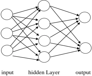
Figure 1: Artificial Neural Network
Figure 2: Non-linear mathematical representation of a neuron in general [1]
F. Long short-term memory
There are a few structures of LSTM units. Typical engineering made of a Cell, the memory part of the LSTM unit and three "controllers," more often called gates, of the stream of data inside the LSTM unit: an input gate, an output gate and a forget gate. A few varieties of the LSTM unit do not have at least one of these doors or perhaps have different entryways. Instinctively, the cell is in charge of monitoring the conditions between the components in the input grouping. The input door controls the degree to which another esteem streams into the cell, the forgot gate controls the degree to which esteem stays in the cell, and the output gate controls the degree to which the incentive in the cell is utilized to process the output actuation of the LSTM unit. The initiation capacity of the LSTM gates is frequently the strategic capacity.
There are associations into and out of the LSTM entryways, a couple of which are intermittent. Loads of these associations, which should be hangingoff amid preparing, decide how the gates work.
Figure 3:The Long Short-Term Memory (LSTM) cell
: Layers
: Pointwise OP
: Copy
The equations for a forward pass of an LSTM are as follows:
it= σg Wixt+ Uiht−1+ bi (5)
ft= σg Wfxt+ Ufht−1+ bf (6)
ot= σg Woxt+ Uoht−1+ bo (7)
ct= ft∘ ct−1+ it ∘ σc Wcxt+ Ucht−1+ bc (8)
ht= ot ∘ σh ct (9)
σg: sigmoid function
σh: hyperbolic tangent function
: denotes the Hadamard productW, U, b: weight matrices and bias vector parameters. xt: input vector
ft: forget gate's vector
it: input gate's vector
ot: output gate's vector
ht: hidden state vector
ct: cell state vector
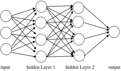
G. Neural Network with hidden Layers (Multi-Layer Perceptron)
An MLP comprises of, something like three layers of hubs: an input layer, an opaque layer, and an output layer. Every center in the input layer is a neuron, utilizes a nonlinear enactment work. MLP uses an administered learning strategy named backpropagation for the training. Its different layers and non-direct initiation recognize MLP from a straight perceptron. It can identify information that is not directly divisible.
Figure 4: A two-layer Neural Network input hidden Layer output
x0
x1 Activation Function (ReLU)
up Output (yp)
x2
. . Summing
. . function
. . ϴ
Threshold
xp
W0
W1
W2
Wp
∑
Φ(.)ht
ct-1
ct
ht-1 ht
xt
X +
X
X σ σ ReLU
ReLU
[image:4.595.360.519.532.663.2] [image:4.595.79.280.657.765.2]Figure 5: A three-layer neural network
1) ReLU - Activation function
The sigmoid is not the main sort of smooth initiation work utilized for neural systems. As of late, a first capacity named Rectified Linear Unit (ReLU) grows into extremely famous because it produces great exploratory outcomes and it never gets flooded with an elevated value of x.
It can be only defined as follows,
f (x) = max (0, x) (10)
IV. RESULTS
The Prediction model for Multi-Currency Exchange Rates based on keras framework of python. After training system repeatedly, the following parameters set for the best results. The ANN and an LSTM use a single hidden layer with twelve and seven neurons. Neural Network with two hidden layers with 50 neurons each. ReLU activation,lecun uniform as kernel initializer, Adam optimizer with a batch size of 16 and 100 epochs for ANN and LSTM. While 20 neurons for Neural Network with two hidden layers with 20 epochs as the datasets used for this work consists of near about 30 – 39 years of data by day and divided into training data and testing data in the 80%-20% proportion since the 1980s till December 2018, the test data is from January 1, 2011, till December 2018, and the following results based on that training dataset.
Table 1.1, Table 1.2 and Table 1.3 shows the correlation matrix using Pearson correlation coefficient method for all the currencies pairs used in the system using complete dataset followed by the heatmap for the same in figure 17.
EUR JPY GBP AUD
EUR 1 0.3694 0.5975 0.3985
JPY 0.3694 1 -0.1702 0.4345
GBP 0.5975 -0.1702 1 0.3746
AUD 0.3985 0.4345 0.3746 1
CAD 0.5702 0.3513 0.3693 0.8446
CHF 0.6359 0.6229 -0.1101 0.7137
CNY -0.3737 -0.2579 -0.0455 0.4526
SEK 0.8193 0.0249 0.6430 0.7520
NZD 0.5993 0.4546 0.4291 0.8765
MXN 0.0519 -0.3736 0.4490 -0.1937 INR -0.2775 -0.4334 0.2943 0.2120
Table1.1: Pearson Correlation Coefficient Matrix
CAD CHF CNY SEK
EUR 0.5702 0.6359 -0.3737 0.8193
JPY 0.3513 0.6229 -0.2579 0.0249 GBP 0.3693 -0.1101 -0.0455 0.6430
AUD 0.8446 0.7137 0.4526 0.7520
CAD 1 0.6082 0.2397 0.7200
CHF 0.6082 1 0.1005 0.2670
CNY 0.2397 0.1005 1 0.5262
SEK 0.7200 0.2670 0.5262 1
NZD 0.7293 0.8332 0.1413 0.5624
MXN -0.1334 -0.6486 0.0350 0.3538 INR -0.0678 -0.6169 0.6971 0.5046
Table1.2: Pearson Correlation Coefficient Matrix
NZD MXN INR
EUR 0.5993 0.0519 -0.2775 JPY 0.4546 -0.3736 -0.4334
GBP 0.4291 0.4490 0.2943
AUD 0.8765 -0.1937 0.2120 CAD 0.7293 -0.1334 -0.0678 CHF 0.8332 -0.6486 -0.6169
CNY 0.1413 0.0350 0.6971
SEK 0.5624 0.3538 0.5046
NZD 1 -0.4166 -0.0846
MXN -0.4166 1 0.9397
INR -0.0846 0.9397 1
[image:5.595.333.519.573.709.2]Table1.3: Pearson Correlation Coefficient Matrix
Figure 17: Heatmap of the Correlation Matrix
Fig 19. USD/JPY Prediction (Jan 2011-Dec2018)
Fig 20. USD/GBP Prediction (Jan 2011-Dec2018)
Fig 21. USD/AUD Prediction (Jan 2011-Dec2018)
Fig 22. USD/CAD Prediction (Jan 2011-Dec2018)
Fig 23. USD/CHF Prediction (Jan 2011-Dec2018)
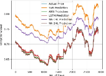
Fig 24. USD/CNY Prediction (Jan 2011-Dec2018)
Fig 25. USD/SEK Prediction (Jan 2011-Dec2018)
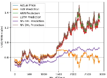
[image:6.595.333.519.66.201.2] [image:6.595.75.263.66.201.2] [image:6.595.78.265.235.372.2] [image:6.595.334.521.237.370.2] [image:6.595.77.263.405.537.2] [image:6.595.337.520.405.537.2] [image:6.595.335.519.573.708.2] [image:6.595.76.263.573.708.2]Fig 27. USD/MXN Prediction (Jan 2011-Dec2018)
Fig 28. USD/INR Prediction (Jan 2011-Dec2018)
[image:7.595.78.262.66.201.2]Table 2.1: R2 scores on Testing Data (Jan 2011-Dec 2018)
Table 2.2: R2 scores on Testing Data (Jan 2011-Dec 2018)
Table 2.3: R2 scores on Testing Data (Jan 2011-Dec2018)
V. CONCLUSION
This paper predicts the exchange rate between world‟s top traded currencies such as USD/EUR, USD/JPY, USD/GBP, USD/AUD, USD/CAD, USD/CHF, USD/CNY, USD/SEK, USD/NZD, USD/MXN and USD/INR from data by day, 30-39 years till December 2018.The above work demonstrates the appropriateness of the Deep learning using SVR, ANN, LSTM and MLP-Neural Networks to the issue of multi-currency exchange rate prediction. The outcomes are profoundly promising; results showed that the average accuracy of the predicting model exceeds 99 %.
REFERENCES
1. Ramadhani Imaniar, Jondri, Rismala Rita, “Prediction of Multi-Currency Exchange Rates Using Correlation Analysis and Backpropagation,” International Conference on ICT for Smart Society Surabaya, 20-21 ISBN: 978-1-5090-1620-4, July 2016.
2. Worasucheep Chukiat, “Forecasting Currency Exchange Rates with an Artificial Bee Colony (ABC) Optimized Neural Network,” International Conference on Advances in ICT for Emerging Regions (ICTer): 324 – 331, 2017.
3. Nanthakumaran P., Tilakaratne C. D., “A Comparison of Accuracy of Forecasting Models: A Study on Selected Foreign Exchange Rates,” Evolutionary Computation (CEC), 2015 IEEE Congress, September 2015.
4. Gao Tingwei, Li Xiu, Chai Yueting, Tang Youhua “Deep Learning with Stock Indicators and Two Dimensional Principal Component Analysis (PCA) for Closing Price Prediction System,” 4673-9904-3/16/$31.00, 2016 IEEE.
5. Rather Akhter Mohiuddin, “Computational intelligence based hybrid approach for forecasting currency exchange rate,” 4799-8349-0/15, 2015 IEEE.
6. Gill S.S., Gill Amanjot Kaur, Goel Naveen, “Indian Currency Exchange Rate Forecasting Using Neural Networks,” 4244-6932-1/10, 2010 IEEE. 7. Chang Jui-Fang, Kuan Chi-Ming, Lin Yu-Wen, “Forecasting Exchange Rates by Genetic Algorithms Based Back Propagation Network Model,” 978-0-7695-3762-7/09, 2009 IEEE.
8. Wang Tien-Chin, KuoSu-Hui, Chen Hui-Chen, “Forecasting the Exchange Rate between ASEAN Currencies and USD,” 4577-0739-1/11, 2011 IEEE.
9. BIS, “Triennial Central Bank Survey - Foreign Exchange Turnover in April 2013: Preliminary Global Result”, Bank Int. Settlements Rev., no. April, p. 24, 2013.
10. Xiaoyun Qu, Xiaoning Kang, Chao Zhang, Shuai Jiang, Xiuda Ma, “Short-Term Prediction of Wind Power Based on Deep Long Short-Term Memory,” 5090-5417-6/16/ $ 31.00 2016, IEEE.
AUTHORSPROFILE
Amit R Nagpuredid Bachelor of Engineering in Computer Engineering from Rashtrasant Tukadoji Maharaj, Nagpur University. Currently pursuing Master of Technology in Computer Science and Engineering from Shri Ramdeobaba College of Engineering and Management, Nagpur, India,IEEE member under Nagpur Subsection under R10 IEEE region, participated in IEEE student website contest, Blind C-coder, completed basic certifications in Data Science from IBM‟s cognitive.ai online portal.
Prediction
Model EUR JPY GBP AUD
SVR 0.9543 0.8729 0.9914 0.9768
ANN 0.983 0.966 0.986 0.970
LSTM 0.991 0.984 0.985 0.997
NN-1HL 0.9967 0.9946 0.970 0.9807
NN-2HL 0.9976 0.9964 0.9942 0.9985
Prediction
Model CAD CHF CNY SEK
SVR 0.9895 -3.3171 -5.3948 0.9837
ANN 0.976 0.792 0.993 0.997
LSTM 0.982 0.649 0.995 0.992
NN-1HL 0.9561 -1.1562 -1.941 0.9946
NN-2HL 0.9989 0.6831 0.991 0.9976
Prediction
Model NZD MXN INR
SVR 0.4926 -0.697 -5.0293
ANN 0.939 0.951 0.963
LSTM 0.969 0.997 0.973
NN-1HL 0.9399 0. 9872 -2.4128
[image:7.595.78.265.236.370.2] [image:7.595.39.270.520.606.2] [image:7.595.65.254.644.731.2]