Obstacle Avoidance and Path Planning for Smart Indoor Agents

Rochester Institute of Technology

RIT Scholar Works

Theses Thesis/Dissertation Collections

7-23-2017

Obstacle Avoidance and Path Planning for Smart

Indoor Agents

Rasika M. Kangutkar

Follow this and additional works at:http://scholarworks.rit.edu/theses

This Thesis is brought to you for free and open access by the Thesis/Dissertation Collections at RIT Scholar Works. It has been accepted for inclusion in Theses by an authorized administrator of RIT Scholar Works. For more information, please contactritscholarworks@rit.edu.

Recommended Citation

Obstacle Avoidance and Path

Planning for Smart Indoor Agents

By

Rasika M. Kangutkar

July 23, 2017

A Thesis Submitted in Partial Fulfillment of the Requirements for the Degree of Master of Science

in Computer Engineering

Approved by:

Dr. Raymond Ptucha, Assistant Professor Date

Thesis Advisor, Department of Computer Engineering

Dr. Amlan Ganguly, Associate Professor Date

Committee Member, Department of Computer Engineering

Dr. Clark Hochgraf, Associate Professor Date

Committee Member, Department of Electrical, Computer & Telecom Engr. Technology

Acknowledgments

I am very grateful towards Dr. Raymond Ptucha for guiding and encouraging me

throughout this study. I acknowledge and hope the best for my teammates: Jacob

Lauzon, Alexander Synesael and Nicholas Jenis. I am thankful for Dr. Ganguly and

Dr. Hochgraf for being on my thesis committee. I thank Suvam Bag, Samuel Echefu

and Amar Bhatt for getting me involved with Milpet. I acknowledge the support my

I dedicate this work to the future lab members working on Milpet, all who supported

Abstract

Although joysticks on motorized wheelchairs have improved the lives of so many,

patients with Parkinson’s, stroke, limb injury, or vision problems need alternate

so-lutions. Further, navigating wheelchairs through cluttered environments without

col-liding into objects or people can be a challenging task. Due to these reasons, many

patients are reliant on a caretaker for daily tasks. To aid persons with disabilities, the

Machine Intelligence Laboratory Personal Electronic Transport (Milpet), provides a

solution. Milpet is an effective access wheelchair with speech recognition capabilities.

Commands such as “Milpet, take me to room 237 or “Milpet, move forward can be

given. As Milpet executes the patients commands, it will calculate the optimal route,

avoid obstacles, and recalculate a path if necessary.

This thesis describes the development of modular obstacle avoidance and path

planning algorithms for indoor agents. Due to the modularity of the system, the

navigation system is expandable for different robots. The obstacle avoidance system

is configurable to exhibit various behaviors. According to need, the agent can be

influenced by a path or the environment, exhibit wall following or hallway centering,

or just wander in free space while avoiding obstacles. This navigation system has

been tested under various conditions to demonstrate the robustness of the obstacle

and path planning modules. A measurement of obstacle proximity and destination

proximity have been introduced for showing the practicality of the navigation system.

The capabilities introduced to Milpet are a big step in giving the independence and

Contents

Acknowledgments i

Dedication ii

Abstract iii

Table of Contents iv

List of Figures vii

List of Tables xii

Acronyms xiii

1 Introduction 2

2 Background 5

2.1 Autonomous Robots . . . 5

2.2 Localization . . . 5

2.2.1 Dead Reckoning . . . 6

2.2.2 Environment Augmentation . . . 6

2.2.3 Innate On-board Localization . . . 8

2.3 Path Planning . . . 10

2.3.1 Djikstra . . . 10

2.3.2 A* . . . 11

2.3.3 D* . . . 13

2.3.4 Focused D* . . . 15

2.3.5 D*Lite . . . 17

2.3.6 Rapidly-exploring Random Trees . . . 18

2.4 Obstacle Avoidance . . . 19

2.4.1 Vector Field Histogram Algorithm . . . 19

2.4.2 VFH+ . . . 22

2.4.3 VFH* . . . 25

2.4.4 Dynamic Window Approach . . . 28

CONTENTS

2.5.1 YOLO . . . 30

2.5.2 YOLOv2 and YOLO9000 . . . 32

2.6 Smart Wheelchairs . . . 34

2.6.1 COALAS . . . 35

2.6.2 MIT’s Smart Chair . . . 35

3 System Overview 37 3.0.1 Milpet . . . 37

3.0.2 Hardware . . . 38

3.0.3 Software . . . 39

3.1 Robot Operating System . . . 41

3.1.1 Useful ROS commands . . . 43

3.2 Gazebo . . . 45

3.2.1 Links and Joints . . . 46

3.2.2 ROS and Gazebo Tutorial: Creating a Robot in Gazebo, con-trolled via ROS . . . 49

4 Human Robot Interaction 66 4.1 Mobile Application . . . 66

4.2 Speech . . . 67

4.3 Voice Feedback . . . 69

5 Obstacle Avoidance 71 5.1 System Integration . . . 71

5.2 Algorithm Development . . . 72

5.2.1 Stage 1: Blocks Creation . . . 72

5.2.2 Stage 2: Goal Heading Direction . . . 76

5.2.3 Stage 3: Block cut-off . . . 76

5.2.4 Stage 3: Behavior Modes . . . 77

5.2.5 Stage 4: Smoothing . . . 80

5.2.6 Stage 5: Lidar Filtering . . . 81

5.2.7 Stage 6: Improving safety . . . 86

5.2.8 Stage 7: Centering the robot . . . 87

5.3 Final Algorithm Overview . . . 87

CONTENTS

6 Path Planning 90

6.1 Algorithm . . . 90

6.2 Mapping . . . 90

6.3 Waypoints . . . 91

6.4 Clusters . . . 93

6.5 Following . . . 96

6.6 System Integration . . . 96

6.7 Centering . . . 97

7 Vision and Lidar Data Fusion 100 8 Results 104 8.0.1 Obstacle Proximity . . . 104

8.1 Obstacle Behavior Modes . . . 104

8.1.1 Encoder Free Mode . . . 110

8.1.2 Testing in Glass Areas . . . 113

8.2 Local Obstacle Avoidance . . . 113

8.2.1 Avoiding Dynamic Obstacles . . . 121

8.3 Reaction Time . . . 122

8.4 Navigation in Autonomous mode . . . 123

8.5 Smart Wheelchair Comparison . . . 129

9 Conclusion 131

10 Future Work 133

List of Figures

2.1 Localization using Landmarks in a Stereo Camera System [1]. . . 7

2.2 Triangulation [2]. . . 8

2.3 Robot Tracking with an Overhead Camera [3]. . . 9

2.4 Possible moves between grid cells [4]. . . 10

2.5 GraphG with costs on edges. . . 11

2.6 A* heuristic h(n) [4]. . . 12

2.7 D* Algorithm. . . 15

2.8 Sample RRT treeT [5]. . . 18

2.9 Certainty grid of VFH [6]. . . 20

2.10 Environment with a robot [6]. . . 21

2.11 Histogram grid (in black) with polar histogram overlaid on the robot [6]. 22 2.12 Polar histogram with Polar Obstacle Densities and threshold [6]. . . . 23

2.13 Candidate Valleys [6]. . . 24

2.14 VFH+: Enlargement angle [7]. . . 25

2.15 a. POD Polar Histogram; b. Binary Polar Histogram; c. Masked Polar Histogram [7]. . . 26

2.16 A confusing situation for VFH+: Paths A and B can be chosen with equal probability. Path A is not optimal, while Path B is. VFH* overcomes this situation [8]. . . 27

2.17 VFH* Trajectories for: a. ng = 1; b. ng = 2; c. ng = 5; d. ng =10 [8]. 27 2.18 Velocity Space: Vr is the white region. [9] . . . 28

2.19 Possible curvatures the robot can take [7]. . . 29

2.20 Objective function for Va ∩ Vs [9]. . . 29

2.21 Objective function for Va ∩ Vs ∩ Vd [9]. . . 30

2.22 Paths taken robot for given velocity pairs [9]. . . 30

2.23 YOLOv1 Example: Image divided into 7× 7 grid. Each cell predicts two bounding boxes (top). Each cell predicts a class given an object is present (bottom) [10]. . . 32

2.24 Image shows bounding box priors fork=5. Light blue boxes correspond to the COCO dataset while the white boxes correspond to VOC [11]. 33 2.25 Smart Wheelchair: COALAS [12]. . . 35

LIST OF FIGURES

3.1 Milpet. . . 37

3.2 Hardware Block Diagram. . . 38

3.3 Teensy microcontroller’s Pin Out. . . 39

3.4 Milpet Hardware. . . 40

3.5 Intel NUC Mini PC. . . 40

3.6 Lidar Sensor: Hokuyo UST 10LX. . . 40

3.7 ROS nodes and topics related to described scenario. . . 41

3.8 System architecture generated by ROS. . . 44

3.9 Screenshot of Gazebo Environment. . . 46

3.10 Revolute joint (left); Prismatic joint (right). . . 47

3.11 Relation between links and joints of a robot model, with reference frames of each joint ref[gazebo]. . . 48

3.12 Gazebo simulation launched via ROS. . . 52

3.13 Gazebo simulation launched via ROS with Willow Garage. . . 53

3.14 Robot created in Gazebo. . . 59

3.15 Gazebo menu to apply torque and force to different or all joints. . . . 60

3.16 Top View of Robot with Visible Lidar Trace, with an Obstacle. . . . 62

3.17 Keys to control the robot in Gazebo. . . 63

3.18 List of ROS topics running during Simulation. . . 64

3.19 Twist messages published to topic cmd vel. . . 65

3.20 Nodes and Topics running during Simulation. . . 65

4.1 Android App Interface. . . 66

4.2 iOS App Interface. . . 67

4.3 Voice out text-to-speech ROS diagram. . . 70

5.1 Avoider node in ROS. . . 72

5.2 Robot’s Lidar scan view up to a threshold. . . 73

5.3 Robot’s Lidar scan view up to a threshold. . . 74

5.4 Different orientation terms associated with Obstacle Avoidance. . . . 75

5.5 Issue with Stage1. . . 76

5.6 Block with blockcutof f. . . 77

5.7 Settingorientationrequired. . . 78

5.8 Block with blockcutof f. . . 81

5.9 Ten raw Lidar scans in the same position. . . 82

5.10 Ten filtered Lidar scans in the same position. . . 83

LIST OF FIGURES

5.12 Lidar scan mapped to Cartesian system, using (5.8), (5.9). . . 84

5.13 Interface for viewing Lidar data on Windows. . . 85

5.14 Setting up IP address for Hokuyo Lidar on Ubuntu. . . 85

5.15 Problem Example: Milpet turning around a corner. . . 86

5.16 Block with Safety Bubbles. . . 87

5.17 Flowchart of Obstacle Avoidance. . . 88

5.18 Obstacle Avoidance System Components. . . 89

6.1 Occupancy Grid that Milpet navigates. . . 91

6.2 Waypoint Example Scenario: Waypoints only at angle changes in path. 92 6.3 Path with Waypoint clusters, and square shaped dilating structire. . . 93

6.4 Path with Waypoint clusters, and diamond shaped dilating structure. 94 6.5 Path with Waypoint clusters going across the corridor. . . 95

6.6 Navigation ROS nodes system. . . 97

6.7 Path with Waypoint clusters going across the corridor. . . 97

6.8 Filter size,fs = 9. . . 98

6.9 Filter size,fs = 15. . . 98

6.10 Filter size, fs = 19. . . 99

6.11 Filter size, fs = 21. . . 99

7.1 Image and Lidar scan data fusion stages. . . 101

7.2 Entire scan -135◦ to 135◦ : Robot is facing right; blue are points from the Lidar; green circle represents the robot; red circle represents a 2 meter radius. . . 102

7.3 Scan cut to -30◦ to 30◦ to match that of the camera. . . 102

7.4 Scan marked up: green shows points belonging to person class; red shows points belonging to no object. . . 103

7.5 Thresholding marked points with distance information. . . 103

8.1 Hallway area that Milpet was tested in. . . 105

8.2 Area explored by Milpet in heuristic mode with no centering. . . 105

8.3 Obstacle Proximity for Fig. 8.2. . . 106

8.4 Area explored by Milpet in heuristic mode with centering on. . . 106

8.5 Obstacle Proximity for Fig. 8.4. . . 106

8.6 Area explored by Milpet in goal mode with centering on andorientationgoal = 0. . . 107

LIST OF FIGURES

8.8 Area explored by Milpet in goal mode with no centering andorientationgoal

= 0. . . 108

8.9 Obstacle Proximity for Fig. 8.8. . . 108

8.10 Area explored by Milpet in goal mode with no centering andorientationgoal = 90. . . 109

8.11 Obstacle Proximity for Fig. 8.10. . . 110

8.12 Area explored by Milpet in encoder free goal mode with centering and orientationgoal = 0. . . 111

8.13 Obstacle Proximity for Fig. 8.12. . . 111

8.14 Area explored by Milpet in encoder free heuristic mode with centering. 112 8.15 Obstacle Proximity for Fig. 8.14. . . 112

8.16 Area explored by Milpet: black points are obstacles detected by lidar; red are undetected obstacles (glass); blue is path of robot. . . 113

8.17 Setup 1 with minimum passage width = 62 inches. . . 114

8.18 Setup 2 with minimum passage width = 50 inches. . . 114

8.19 Obstacle Avoidance in Setup 1 with heuristic mode and centering on. 115 8.20 Obstacle Proximity for Fig. 8.19. . . 115

8.21 Obstacle Avoidance in Setup 2 with goal mode and centering on. . . . 116

8.22 Obstacle Proximity for Fig. 8.21. . . 116

8.23 Obstacle Avoidance in Setup 2 with goal mode and no centering. . . . 117

8.24 Obstacle Proximity for Fig. 8.23. . . 117

8.25 Obstacle Avoidance in Setup 2 with heuristic mode and centering on. 118 8.26 Obstacle Proximity for Fig. 8.25. . . 118

8.27 Obstacle Avoidance in Setup 2 with heuristic mode and no centering. 119 8.28 Obstacle Proximity for Fig. 8.27. . . 119

8.29 Human driving manually through Setup 2. . . 120

8.30 Obstacle Proximity for Fig. 8.29. . . 120

8.31 Different angles of approach. . . 122

8.32 Reaction time when a sudden obstacle blocks Milpet’s entire path. . . 123

8.33 Autonomous traveling with w = 13 ft and ds = 3 × 3 sq. ft. . . 124

8.34 Path explored for Fig.8.33. . . 124

8.35 Obstacle proximity for path in Fig.8.33. . . 125

8.36 Autonomous traveling with w = 10 ft and ds = 4 × 4 sq. ft. . . 125

8.37 Autonomous traveling with w = 10 ft and ds = 3 × 3 sq. ft. . . 126

8.38 Path explored for Fig.8.37. . . 126

LIST OF FIGURES

List of Tables

2.1 Relation between speed of model and distance travelled by vehicle. . . 32

3.1 Useful ROS commands. . . 43

3.2 ROS Topic Rates. . . 45

3.3 Different types of joints. . . 47

3.4 Relation between links and joints of a robot model. . . 48

3.5 Robot Link Details . . . 54

3.6 Robot Joint Details. . . 54

4.1 Speech Recognition speed (in seconds). . . 69

4.2 Dialogue Scenario with Milpet. . . 70

5.1 Obstacle Avoidance Behavior Modes. . . 79

8.1 Robot Reaction for Dynamic Obstacles. . . 121

8.2 Destination Proximity. . . 128

Acronyms

COALAS

COgnitive Assisted Living Ambient System

DWA

Dynamic Window Approach

GPS

Global Positioning System

IoU

Intersection over Union

mAP

mean Average Precision

MIL

Machine Intelligence Lab

Milpet

Machine Intelligence Lab Personal Electric Transport

MIT

Massachusetts Institute of Technology

MOI

Acronyms

PASCAL

Pattern Analysis, Statistical Modeling and Computational Learning

PC

Personal Computer

POD

Polar Obstacle Density

ROS

Robot Operating System

RPN

Region Proposal Network

RRT

Rapidly Exploring Random Tree

sdf

Simulation Description Format

urdf

Universal Robotic Description Format

VFH

Vector Field Histogram

VOC

Acronyms

xacro

XML Macros

YOLO

You-Only-Look-Once

YOLOv2

Chapter 1

Introduction

With the boom in autonomous robots, navigation to a destination while avoiding

obstacles has become important. This thesis focuses on making a modular obstacle

avoidance system linked up with path planning. The obstacle avoidance system can

be easily configured to suit different differential drive robots to exhibit different

be-haviors. The robot can be influenced by a path, environment, exhibit wall following

or hallway centering, or display a wandering nature.

Part of the motivation behind this study is for making the Machine Intelligence

Lab Personal Electric Transport, Milpet, autonomous. Milpet is equipped with a

single channel Lidar, an omni-vision camera, sonar sensors, encoders and a front facing

camera. Milpet is an effective access wheelchair that is aimed at helping patients with

vision problems, Parkinson’s or any patient, who cannot make use of the joystick for

efficient navigation. Avoiding obstacles or maneuvering in cluttered environments

can be a challenge for such patients. Milpet is speech activated and commands like

“Milpet, take me to Room 237”, or “Milpet, take me to the end of the hallway”, can

be given. These commands invoke the path planning system, which then guides the

obstacle avoidance system in which direction to go. Milpet thereby helps patients in

navigating their household and regaining their privacy and independence.

Since the target deployment areas are assisted living facilities such as hospitals,

CHAPTER 1. INTRODUCTION

building a separate map of the environment through Simultaneous Localization And

Mapping (SLAM), we can use static floor plans and convert them to occupancy grids.

The global path of the robot comes from the global path planning module which

is based off of D* Lite [14]. Here the path planning module acts at a global level

pro-viding waypoints and directions to the obstacle avoidance system. While navigating

from location A to location B, the obstacle avoidance system ensures the patient’s

and other’s safety. The You-Only-Look-Once framework version 2 [11], YOLOv2, is

a real-time object detector and recognizer that can make Milpet more interactive and

smarter with people. This vision information can be integrated into the system as

well, and has been tested off the robot

Milpet is a research platform in the Machine Intelligence Lab and is continuously

being improved. Making the navigation system modular makes it easier for testing

different concepts and behaviors, and expanding it to use various sensors. The Robot

Operating System (ROS) is made use of for building the code base. All code is written

in Python, which is a scripting language that is easy to understand and modify.

The main challenge of this work was to make use of the onboard sensors to create

an optimized navigation system. Milpet has been tested in an academic building in

varying scenarios. The obstacle avoidance system has been tested with and without

paths to demonstrate its effectiveness. An evaluation measurement of obstacle

prox-imity and destination proxprox-imity have been introduced for showing the practicality of

the obstacle avoidance and navigation systems.

The main contributions of this work include:

• Modular obstacle avoidance algorithm

• Path planning and guiding algorithm

• Gazebo test platform for Milpet

CHAPTER 1. INTRODUCTION

• Interaction interface setup between user and Milpet via speech

• Evaluation metric: obstacle proximity

• Evaluation metric: destination proximity

This thesis is organized as follows: The background chapter talks about the

ba-sics of obstacle avoidance, path planning, localization techniques, object recognition

frameworks and an overview on other smart wheelchairs. The system overview

chap-ter briefly goes over Milpet’s hardware and software used. The following chapchap-ters

describe the interaction capabilities of the robot, the obstacle avoidance algorithm

development and the path planning system. This study is then rounded up with the

Chapter 2

Background

2.1

Autonomous Robots

For a robot to be termed as truly autonomous, the robot must be able to solve the

following questions: “Where am I?”,“Where to go?’ and “How to get there?” [15].

The foremost question, is concerned with determining where a robot is on a given

map; this is termed as localization. “Where to go?” represents the destination where

the robot wants to go. This can be answered by input from different interfaces; for

example: “Go to the kitchen”, is a speech command, where the wordkitchen should

be deduced as the destination, and mapped to a position on the map. The final

question, “How to get there?”, embodies the robots capability of planning a path

to the destination and avoiding obstacles to get there. In the following sections,

localization, path planning, obstacle avoidance, etc. are discussed; giving an overall

base on what algorithms can be used, to make a robot autonomous.

2.2

Localization

Localization answers the question: “Where am I?”. The term localizatoin refers to

figuring out where a robot is on a given map. A robot’s position, is characterized

by x, y, z, φ in space, where x, y, z ∈ Cartesian Space and φ is the orientation of the

CHAPTER 2. BACKGROUND

There are various methods for carrying out localization. Global Positioning

Sys-tem (GPS) is a popular outdoor localization technique. However, GPS has an

accu-racy of 2-8 meters [16]; thus, it is not suitable for indoor robots.

2.2.1 Dead Reckoning

Dead reckoning calculates the displacement and orientation of a robot along X, Y

and Z axes from the initial position. Using geometry and a robot’s configuration

and dimensions, the position of the robot can be determined. This method depends

heavily on its sensors, and is susceptible to noise, systematic and non systematic

errors. Encoders that measure the number of revolutions of each wheel, is one kind of

sensor that is used for dead reckoning. One challenge in dead reckoning is determining

the initial position.

2.2.2 Environment Augmentation

Many localization techniques add sensors or markers to the environment, to facilitate

in determining where the robot is. Making changes to the environment, by adding

markers, sensors or tracks comes under this category.

2.2.2.1 Artificial Landmarks

These are markers or labels that are positioned at particular known locations. When

the robot is able to sense one of these markers, it can calculate the distance from the

marker and deduce where it is. This is because, it already knows the real size of the

marker and through comparison between the real and perceived dimensions, it can

determine the angle and how far it is from the marker. Figure 2.1 shows a flowchart

CHAPTER 2. BACKGROUND

Figure 2.1: Localization using Landmarks in a Stereo Camera System [1].

2.2.2.2 Triangulation

Triangulation makes use of readings, R, from three or more sensors. An outdoor

example of triangulation is GPS; it makes use of three satellites to pinpoint a position.

For indoor environments, instead of using satellites, sensors like: beacons or even

Wireless Fidelity (WiFi), are used. The strength of signals from three sensors is used

to determine where it is on the map. Beacons emit continuous signals in a radial

manner. The strength of the signal is inversely proportional to the distance from the

beacon. Thus, the position of the robot can be determined from the strength of signals

w.r.t. the known positions of each beacon. Figure 2.2 shows how triangulation using

sensors work. R is the readings returned to the system, which helps in determining

CHAPTER 2. BACKGROUND

Figure 2.2: Triangulation [2].

2.2.2.3 Following and Tracking

One of the simplest kinds of localization is to have the robot follow a line; the line

can be painted on, or even be magnetic. By following the line, the robot’s position

can always be known.

Another method for localizing a robot, is to track the robot in its environment.

One way of doing this is to install an overhead camera in an environment. The camera

can then determine the robot’s position w.r.t. the environment. This technique is

made use of in Automated Guided Vehicles (AGV) and in swarm robotics. Figure 2.3

(left) shows an image captured by an overhead camera; Figure 2.3 (right) shows the

detected positions and orientations of the robots, the white line depicts the heading

of the robot.

2.2.3 Innate On-board Localization

All the above methods, albeit for dead reckoning, rely on changing the environment

CHAPTER 2. BACKGROUND

Figure 2.3: Robot Tracking with an Overhead Camera [3].

running out, affect the entire localization system. So, if any of these methods are

made use of, ways to check and maintain these augmentations must be carried out.

Instead of relying on these external paraphernalia, the robot can be trained with

machine learning techniques to help in localization; this would require no need of

adding accessories to the environment.

2.2.3.1 Machine Learning

Localization using machine learning depends on having data with unique

signa-tures/features at different positions. Data from the robot’s sensors is collected at

different positions, with the x, y positions as ground truths and fed to a classifier.

The classifier is then trained and tested on a held out data-set that the robot has

never seen. The accuracy of the system can then be calculated.

The classifier used can be trained using different techniques; Support Vector

Ma-chines, Decision Trees, Random forest, Convolutional Neural Networks are a few types

of classifiers. Some machine learning techniques have a prerequisite step to training:

feature extraction, where techniques like Histogram of Gradients (HOG) [17], Scale

Invariant Features Technique (SIFT) [18] and data dimension reduction techniques

CHAPTER 2. BACKGROUND

2.3

Path Planning

Searching for a goal location is an integral part of robotics. The initial position of

the robot is termed as the start / source, while the end position is termed as the

destination / goal. The terrain the robot is to navigate is generally represented as a

grid.

Planning a path from the start to the destination is dependent on the map

rep-resentation. The map can be represented in a topological form or metric form. In

the metric form, objects, walls, etc. are placed in a two-dimensional space, where

each position on the map represents a real area to scale. This is the most common

type of map. Topological maps represent specific locations as nodes and the distances

between them as edges connecting the nodes, making them graphs.

Figure 2.4: Possible moves between grid cells [4].

Figure 2.4 shows the relation between cells in the map. Each cell has at most

eight neighbors. Since the terrain is known, informed search algorithms like Djikstra,

A*, D* are used. These algorithms make use of an evaluation criteria, to find the

optimal path. In this section various path planning techniques are described.

2.3.1 Djikstra

In 1956, the Djikstra path planning technique was formulated by Edsger W. Djikstra

[19]. In the Djikstra algorithm, a graph G is considered with n nodes via edges e.

CHAPTER 2. BACKGROUND

visited list V and unvisited list U. s is the start node, g is the goal node. U is a

min-priority queue.

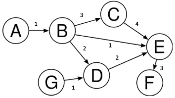
Figure 2.5: GraphG with costs on edges.

First, s is placed in U with es,s = 0; no cost is incurred. The other nodes are

added toU withes,n1...k =∞, wherek is the number of nodes in the graph. FromU,

the node which has the minimum cost is chosen. In this case, the start node is picked,

and costs from the start s to its neighbors x are updated. The rule for updating the

cost forxis shown in (2.1), whereecurrent refers toxcost inU andx−1 is the current

node being considered. After updating the costs to each neighbor, the selected node

(start node) is removed from U and placed in V. The same steps are repeated until

g is added to V or if the minimum cost in U is ∞, i.e. no path to g found.

es,xupdated =min(es,xcurrent, es,x−1+ex−1,x) (2.1)

2.3.2 A*

The A* search algorithm is an extension of Djikstras algorithm and was proposed in

1968. It makes use of an evaluation function with a heuristic , (2.2), to get better

performance. A* is a very popular algorithm in robotics and path planning.

f(n) = g(n) +h(n) (2.2)

CHAPTER 2. BACKGROUND

to the goal node g. g(n) and gs,n, both represent the cost from the start node s to

n. Figure 2.6 shows how the estimate is determined. Since A* never overestimates

the cost to the goal g, the shortest path can always be found. Referring to the grid

cell structure in Figure 2.4, diagonal edges have a cost cof 1.4, while horizontal and

vertical edges have a cost c of 1. For example, cx1,x9 = 1.4 and cx1,x4 = 1. Ifx2 and

x7 are obstacles, then cx1,x2 = ∞ and cx1,x7 = ∞. The notation b(x1) = x2 shows that cell x2 is the back-pointer b of x1.

Figure 2.6: A* heuristich(n) [4].

Two lists are maintained here as well: Open list queue O and Closed C list.

Algorithm 1 describes the A* algorithm. Line 1 shows that initially, s is added to

O. Lines [2-4] says that if O is empty, then the algorithm is stopped, else node with

the least f(n), f(nbest) is popped from the queue and nbest is added to C. Lines

[8-12] show that if nbest is equal to g then the path is found, else the neighbors x /∈

C are added to O. If x is already present in C and gs,nbest+cnbest < gx then update

CHAPTER 2. BACKGROUND

Algorithm 1: A* Psuedocode.

1 O ← s;

2 while n_best 6= g OR O not empty do 3 f(n_best)= min(f(n_i)),i∈ O ;

4 C ← nbest;

5 if n_best == g then

6 exit();

7 else

8 for each x neighbor ofn_best do

9 if x /∈C then

10 if x∈O then

11 g_s,x=min(g_s,x,g_s,nbest+g_nbest,x) ;

12 O ←x;

2.3.3 D*

A* and Djikstra algorithms assume that the entire environment is known between

planning, however, this is seldom the case. Paths can get blocked off, new and/or

moving obstacles may be present. To encompass this, D* was proposed in [20]. The

term D* comes from Dynamic A*, as it aims at efficient path planning for unknown

and dynamic environments. If a robot is following a path provided by A*, and a

change in the surroundings is encountered by the robot, A* can be called again;

with the robots current location as the start point s. However, this recalculation is

expensive and doesnt make use of the former calculations made, while finding the

path. Further, by the time the robot recalculates this new path, the robot may have

gone along a wrong path. For this reason, a faster and more efficient method for

recalculating paths arises, and D* aims at addressing it.

Unlike A*, D* calculates the path starting from the goal g to the start s. In D*,

each grid-cell has h(x), p(x) and b(x), which represent the estimated cost from goal

g tox, the previous calculatedh(x) and a back-pointer. The back-pointer represents

CHAPTER 2. BACKGROUND

CLOSED, N EW states t, depending on whether it is, hasnt been or was added to

the open list O, respectively.

h(Y) =h(X) +c(X, Y) (2.3)

k(X) =min(h(X), p(X)) (2.4)

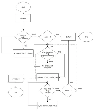
For implementing D*, initially all cells have state t(deg) set toN EW, the goal is

g is placed on the open list O and the cost h(g) is set to zero. P ROCESS ST AT E

and M ODIF Y COST are the two main functions here. O is a min-priority queue,

where the cell with the smallest keykmin is removed first. k for each cell is calculated

using (2.4). c(x, y) is the cost of moving from x to y cells. kold is thek of the most

recent removal of top element x, from O. Figure 2.7 and Algorithm 2 describe the

flow chart of D* and P ROCESS ST AT E pseudo-code, respectively. The following

are the conditions checked for each neighborY of current cell X:

1. if neighbor Y, witht(Y) = CLOSEDV

h(Y)< kold V

h(X)> h(Y) +c(Y, X)

2. if neighbor Y has t(Y) =N EW

3. if neighbor Y has b(Y) =XV

h(Y)< p(Y)

4. if neighbor Y has b(Y)6=XV

h(Y)> h(X) +c(X, Y)

5. if p(X)>=h(X)

6. if neighbor Y has b(Y)6=XV

h(X)> h(Y) +c(Y, X)V

h(Y)> kold V

h(Y) =

p(Y)

If Condition 1 is true, h(x) is set to h(Y) +c(Y, X) . For Condition 2, the new

CHAPTER 2. BACKGROUND

using (2.3). For Condition 3, if X is either OP EN or CLOSED, p(Y), h(Y) are

updated andY is added toO. When Condition 4 is satisfied, Condition 5 is checked.

If it is true, the back-pointer b(Y) = X is set, andp(X) is updated accordingly. Y is

then added to the list O. Y is inserted into O, if Condition 6 is satisfied.

Figure 2.7: D* Algorithm.

D* is thus, capable of repairing and replanning, to get to the goal g.

2.3.4 Focused D*

The number of steps in D* are many. Focused D* [21] reduces the number of steps by

CHAPTER 2. BACKGROUND

Algorithm 2: D* P ROCESS ST AT E Psuedocode.

1 X =dequeue(O);

2 if X =N U LL then 3 return -1;

4 k_old =get k_min();

5 for each neighbor Y of X do 6 if Condition1then

7 b(X) = Y;

8 h(X) = h(Y) +c(Y, X);

9 for each neighbor Y of X do 10 if Condition2then

11 enqueue(Y);

12 h(Y) = h(X) +c(X, Y);

13 b(Y) =X;

14 else

15 if Condition 3 then

16 if t(X) =OP EN then

17 if h(Y)< p(Y)then

18 p(Y) =h(Y);

19 h(Y) =h(X) +c(X, Y);

20 h(Y) = p(Y) = h(X) +c(X, Y);

21 enqueue(Y);

22 else

23 else

24 if Condition4then 25 if Condition5then

26 b(Y) = h(X);

27 h(Y) =h(X) +c(X, Y);

28 if t(Y) =CLOSED then

29 p(Y) =h(Y);

30 enqueue(Y);

31 else

32 p(X) =h(X);

33 enqueue(X);

34 else

35 if Condition6then

36 p(Y) =h(Y);

CHAPTER 2. BACKGROUND

of the goal. Equation 2.5 describes the updated cost function for h(Y).

h(Y) =h(X) +c(X, Y) +φ(X, s) (2.5)

2.3.5 D*Lite

D* Lite [14] has the same output as D*, but is done is lesser steps. D* lite has no

back-pointers. Each cell on the grid, xhas ag(u) andrhs(u) value. Ifg(u) = rhs(u)

then, uis said to be consistent, else it is inconsistent. Inconsistent cells are added to

a priority queue U. A cell is termed as over-consistent if g(u) > rhs(u) and

under-consistent if g(u)< rhs(u). The priority, k, is calculated using (2.6). When adding

u to U, the function U P DAT E V ERT EX() is called. Here, if u∈U, it is removed

fromU and if the neighbor is inconsistent, it is added to the queue along with its key

k.

k =min(g(u), rhs(u) +h(u)) (2.6)

rhs(u) =minn∈N eighbors(g(n) +c(u, n)) (2.7)

To start the algorithm, all g(deg) and rhs(deg) are initialized to ∞. Only

rhs(goal) is set to zero and added toU. After thisCOM P U T E SHORT EST P AT H()

is called. In the functionCOM P U T E SHORT EST P AT H(), whilektop ofU is less

than the kstart or rhs(start)! =g(start) the function runs. The top most element, u

is dequeued. Ifuis over-consistent,g(u) =rhs(u) and theU P DAT E V ERT EX() is

called for all neighbors. Ifuis consistent, theng(u) is set to∞andU P DAT E V ERT EX()

is called on u, itself, as well as its neighbors.

Once the path is calculated, the robot moves along the path. If any discrepancy

CHAPTER 2. BACKGROUND

and U P DAT E V ERT EX() is called on u. Also, for every member in U, the cost

is updated with (2.7). Following this, COM P U T E SHORT EST P AT H() is called

again.

2.3.6 Rapidly-exploring Random Trees

A Rapidly-exploring Random Tree (RRT) is a tree structure constructed from

ran-domly sampled waypoints for path planning. With states X, a tree is made, from

the start position xroot to xgoal, where X ∈Xf ree. States can be either f ree or have

an obstacle. The algorithm continues until xgoal is reached, or until the maximum

number of iterations,max, are completed.

Figure 2.8: Sample RRT treeT [5].

Algorithm 3 describes the steps of building an RRT,T. First, the root node,xroot,

is added to T, and a point xrandinX is randomly sampled. The closest point xnew to

xroot in the direction of p is considered, with maximum distance stepsize away from

xroot. If xnew∈Xf ree, thenxnewis added to the tree T; if not,xnew is discarded and

CHAPTER 2. BACKGROUND

Algorithm 3: RRT Psuedocode.

1 T ← xstart;

2 while x_goal ∈/ T OR i6=maxdo 3 Sample point x_rand;

4 xnear ←closest point(T, xrand);

5 x_new =get new point(x_near, stepsize); 6 if x_new∈X_{f ree} then

7 T ←xnew;

8 else

9 discard x_new;

2.4

Obstacle Avoidance

Avoiding obstacles while navigating is an important component of autonomous

sys-tems. Robots must be able to navigate their environment safely. Obstacle avoidance

is more challenging than path planning. Path planning requires one to go in the

direction closest to the goal, and generally the map of the area is already known.

On the other hand, obstacle avoidance involves choosing the best direction amongst

multiple non-obstructed directions, in real time. The following sections briefly discuss

common obstacle avoidance algorithms.

2.4.1 Vector Field Histogram Algorithm

The vector field histogram method [6] is a popular local obstacle avoidance

tech-nique for mobile robots. The main concepts included in the VFH algorithm are the

certainty/histogram grid, polar histogram and candidate valley.

The area surrounding the robot, is represented as a grid. When an obstacle

is detected by the sensor at a Cartesian position (x,y), the values in the grid are

incremented. Here the grid acts like a histogram and is called a Cartesian histogram.

Thus, for sensors prone to noise, this histogram grid aids in determining exact readings

CHAPTER 2. BACKGROUND

Figure 2.9: Certainty grid of VFH [6].

cells with numerals, show where an obstacle is present. The higher the number, the

more probable it is that an obstacle is there.

Once this grid is evaluated, it is collapsed into a polar histogram, which is one

dimensional vector representation centered around the robot. It represents the polar

obstacle density (POD). Figure 2.10 shows the top view of an environment, with a

pole and walls. Figure 2.11 shows the certainty histogram with the polar histogram

overlaid on it and Figure 2.12 c. shows the same polar histogram with degrees along

the X axis and POD along the Y axis.

Depending on the density level of obstacles, free/safe areas, termed as candidate

valleys, are determined and then the robot selects the optimal one. The candidate

valleys are determined as areas with POD lesser than the threshold. Figure 2.13

depicts the candidate valleys.

CHAPTER 2. BACKGROUND

Figure 2.10: Environment with a robot [6].

this, if there is more than one candidate valley, the one which contains the target

direction is chosen and the robot steers in this direction. To avoid getting close to

CHAPTER 2. BACKGROUND

Figure 2.11: Histogram grid (in black) with polar histogram overlaid on the robot [6].

2.4.2 VFH+

The essence of VFH is described in the previous paragraphs. After the original VFH

algorithm was proposed, it was revised and further improved to formulate VFH+ and

VFH*.

In VFH+ [7], the concepts of considering the dynamics of the robot, enlargement

angle, masked and binary polar histograms were added. Every obstacle is dilated by

gamma to avoid collision with it. Equation (2.8) shows how gamma is calculated.

rr +s = rr +ds where rr is the robot radius and ds is the minimum distance to

CHAPTER 2. BACKGROUND

Figure 2.12: Polar histogram with Polar Obstacle Densities and threshold [6].

distance to the obstacle. Figure 2.14 depicts the relevancy of the enlargement angle.

γ =arcsin(rr+s/d) (2.8)

In the original VFH algorithm, the robot is assumed to be able to change its

direction immediately. VFH+ considers the dynamics and kinematics of the robot and

the minimum left and right turning radii (symbols) are calculated. Knowingrl andrr,

the possibility of collision with obstacles can be determined before attempting to turn.

If a collision is foretold, the area is termed as blocked, else free. This creates a new

masked polar histogram. Figure 2.15 shows the original polar histogram described in

VFH, the binary polar histogram that VFH uses and the improved masked histogram

in VFH+.

CHAPTER 2. BACKGROUND

Figure 2.13: Candidate Valleys [6].

the VFH algorithm. In VFH, the center of the candidate valley is chosen as the

direction to steer in. Now, a margin of s is added, where s represents the size of

sector required for the robot to fit. Candidate valleys are further divided into two

categories: narrow and wide. Candidate valleys greater in width than parameter

smax are termed as wide, else termed as narrow. If the selected candidate valley is

narrow, 2.9 describes how the candidate direction cs is chosen.

cs = (kr+kl)/2 (2.9)

For wide candidate valleys, (2.10), (2.11) describe how the margin limits of the

CHAPTER 2. BACKGROUND

Figure 2.14: VFH+: Enlargement angle [7].

direction cs is chosen.

cl = (kl)−smax/2 (2.10)

cr = (kr) +smax/2 (2.11)

cs = (cr+cl)/2 (2.12)

Here kl and kr correspond to left and right limits of the candidate valley.

2.4.3 VFH*

VFH+ considers the best local direction to go in. Due to this, it is possible for VFH+

CHAPTER 2. BACKGROUND

Figure 2.15: a. POD Polar Histogram; b. Binary Polar Histogram; c. Masked Polar Histogram [7].

this doesnt happen, while navigating towards a goal. The name VFH* comes from

the fact that VFH+ is combined with A* 2. Figure 2.16 shows a confusing situation

for VFH+. Black areas are obstacles, gray areas are the enlarged obstacles and white

denotes free space. The figure depicts two directions the VFH+ algorithm may take,

with a fifty-fifty chance. If path A is taken, the robot will get stuck. To avoid this,

the projected VFH+ directions are evaluated in VFH*.

VFH+ provides primary candidate directions to go in from the polar histogram.

VFH* uses these and envisages the robot’s position and orientation after a step ds.

Following this, VFH+ is applied to find the subsequent projected candidate directions

for these new positions. This process is done ng times recursively, in a breadth

first search fashion. A node in the graph represents the position and orientation of

CHAPTER 2. BACKGROUND

Figure 2.16: A confusing situation for VFH+: Paths A and B can be chosen with equal probability. Path A is not optimal, while Path B is. VFH* overcomes this situation [8].

candidate direction that leads to the goal node with the least cost is selected. Cost

is assigned to each node in the graph according A* heuristics. Figure 2.17 shows the

chosen branch for varying values of ng.

CHAPTER 2. BACKGROUND

Figure 2.18: Velocity Space: Vr is the white region. [9]

2.4.4 Dynamic Window Approach

The DWA algorithm [9] determines the required linear velocity,v, and angular

veloc-ity, ω for the robots dynamics. The velocity pair, < v, ω¿, is determined by finding

the intersection betweenVs,VaandVd. Vs are admissible velocity pairs that the robot

can reach. Va are velocity pairs where the robot can satisfy (2.13) before hitting any

obstacle. Finally, the dynamic window is considered for time t. Velocity pairs that

the robot can reach considering the linear acceleration αv and angular acceleration

αω give Vd. Figure 2.18 shows the admissible velocity pairsVr in white.

Vr =Vs∩Vd∩Va (2.13)

G(v, ω) =σ(α∗heading(v, ω) +β∗dist(v, ω)γ∗velocity(v, ω)) (2.14)

With the defined Vr space, the velocity pair that maximizes Eq. () is set as the

velocity pair for the robot. α, β,γ are hyper parameters that adjust the importance

CHAPTER 2. BACKGROUND

Figure 2.19: Possible curvatures the robot can take [7].

orientation. distgives the distance to the closest obstacle. The closer the obstacle is,

the smaller this term becomes. The velocity term is a measure of the progress along

the curvature. The objective functions for Va ∩ Vs and Va ∩ Vs ∩ Vd are shown in

Figure 2.20 and Figure 2.21 respectively. The vertical line denotes the maxv, ω pair.

Figure 2.20: Objective function forVa ∩ Vs [9].

ap-CHAPTER 2. BACKGROUND

Figure 2.21: Objective function forVa ∩Vs ∩Vd [9].

propriate velocities. Figure 2.22 shows the behavior of a robot at different velocity

pairs.

Figure 2.22: Paths taken robot for given velocity pairs [9].

2.5

Object Detectors

2.5.1 YOLO

The You-Only-Look-Once (YOLO) framework [10] is a real-time object detector and

recognizer. It runs at 45fps. YOLO is trained to classify 20 different classes, belonging

to PASCAL VOC 2007 [22]. To evaluate the performance of the classifier, the mean

CHAPTER 2. BACKGROUND

mean Average Precision (mAP). YOLO’s performance is 64.4 mAP for the twenty

classes.

Other object detectors like R-CNN [23], break down object detection and

recog-nition into parts. The first step gets candidate regions using methods like selective

search. This is termed as a region proposal network (RPN) and outputs

bound-ing boxes where objects are likely to be present. These region proposals are then

passed through a classifier. Post-processing involves merging overlapping bounding

boxes, removing duplicate boxes and re-scoring. Since each of these systems, RPN,

classification and post-processing are separate, it is harder and slower to train. Also,

unlike humans, these detectors take multiple passes at the image before giving its final

output, allowing them to run at 5-18fps, which is too slow for real time applications.

With a single pass, a human can distinguish a variety of objects. YOLO takes

inspiration from this, and aims at making its net not deeper, but the concept easier

to learn. Instead of breaking down the task into object detection followed by object

recognition, a single network is used. Images are divided into a grid of 7×7. Each cell

predicts two bounding boxes. Each bounding box predicts how confident it is that an

object is present within it,P(Object). Also, the bounding box itself, has a confidence

level. This makes the network learn to predict better bounding boxes per cell. The

image is also spatially divided, where each cell predicts which class is present, given

an object is present, P(class|Object). Using this, along with the bounding boxes

above the threshold, a label is given to the bounding box.

The classifier learns to predict better bounding boxes and generalizes to which

objects occur together. YOLO makes use of DarkNet [24] for training.

Having a real-time object detector and recognizer can be used in many different

application areas. Self - driving cars and robots can make use of these to improve

their understanding of the world and react immediately. [25], illustrates the relation

CHAPTER 2. BACKGROUND

Figure 2.23: YOLOv1 Example: Image divided into 7× 7 grid. Each cell predicts two bounding boxes (top). Each cell predicts a class given an object is present (bottom) [10].

of 60mph. Table 2.1 shows the relation between speed of the classifier (fps) and the

speed of the vehicle, with the distance traveled by the car.

Table 2.1: Relation between speed of model and distance travelled by vehicle.

Model Speed Distance (in ft) mAP

R-CNN 0.05fps 1742.4 66

Fast R-CNN 0.5fps 176 20

Faster R-CNN 7fps n 12 73.2

YOLO 45fps 3 63.4

2.5.2 YOLOv2 and YOLO9000

The next iteration of YOLO makes several improvements to make it better, faster and

stronger [11]. Making use of batch normalization, the mAP went up by 2%. Batch

normalization helps to regularize the model, making it generalize better and prevent

CHAPTER 2. BACKGROUND

higher resolution images, such as 448×448 pixels, better filters were learned. Taking

inspiration from RPN, instead of predicting co-ordinates of the bounding box in the

final layer, offsets from the cell are determined. Each bounding box now predicts class

and object predictions. Object prediction is the intersection over union (IOU) of the

ground truth and bounding box. IOU is the ratio of the overlapping area between

the predicted and ground truth bounding boxes over the union of the area of the

two boxes. The class prediction is the probability of a class given that an object is

present. Providing priors for bounding boxes can make the detector better. To get

these priors, k-means clustering was run on the training data. Figure 2.24 shows the

priors calculated. k=3 was chosen for YOLO9000 and k=5 for YOLOv2.

Figure 2.24: Image shows bounding box priors for k=5. Light blue boxes correspond to the COCO dataset while the white boxes correspond to VOC [11].

YOLO has two losses, one related to the bounding box prediction (object

detec-tion) and one related to the class (object recognidetec-tion). Ground truths for the object

detection part are limited however that for object recognition is generally more. For

example, there are many images with bounding boxes provided for dog but few that

would give the bounding box for a Dalmatian. However, there are many examples of

CHAPTER 2. BACKGROUND

between labels, the object detection pipeline can be provided with more data and the

model can learn to predict new classes. YOLOv2 performance improves to 76.8mAP

at 40fps for 544 × 544 pixel images.

Considering YOLOv2s accuracy and speed, for this work, YOLOv2, trained on

the COCO dataset with 80 classes has been used.

2.6

Smart Wheelchairs

A smart wheelchair is an electric wheelchair, to which changes have been made to

control the motors via software, or an autonomous robot upon which a chair has been

mounted. Research and innovation in smart wheelchairs has been ongoing since 1986

[26]. Smart wheelchairs aim at supporting a specific niche of wheelchair users: users

with vision issues, tremors, cerebral palsy, etc. Smart wheelchairs can exhibit one or

more of the following capabilities [26]:

• Travel to a destination while avoiding obstacles

• Avoid obstacles while user controls main directions to go in

• Follow a wall at a fixed distance

• Pass through door ways

• Follow a path already traveled by the robot

• Rewind movements taken by robot up to starting spot

• Follow or go up to a moving or stationary object.

• Plan and follow a line through environment with intersections.

• Turn on spot or make a K-turn

The following sections go over a few smart wheelchairs and the technology they

CHAPTER 2. BACKGROUND

2.6.1 COALAS

The COgnitive Assisted Living Ambient System [12] is a smart wheelchair equipped

with an omni-directional camera, twelve infrared sensors, eleven sonars, Arduino

boards, a microphone and encoders. COALAS makes use of the Robot Operating

System for system integration. The wheelchair avoids obstacles by fusing input from

Figure 2.25: Smart Wheelchair: COALAS [12].

its sonar sensors and joystick. An artificial potential field is created, making it avoid

obstacles and go in the general direction given by the user via the joystick.

COALAS makes use of geo-localization; it is driven along all the possible paths it

can take, during which, the omni-directional camera takes photos and stores them.

Feature matching between the perceived images and stored photos, using SIFT, is

carried out when traveling along a previously driven path.

2.6.2 MIT’s Smart Chair

Research at MIT for smart chairs delves into making the robot recognize different

locations on its own. The smart chair at MIT aims at acting as a tour guide [27].

Initially, it follows a human guide through MIT; the person narrates and describes

different areas within the building [13]. The robot then interprets the spoken

CHAPTER 2. BACKGROUND

2.26 shows an example case of locations on a map. The pie charts denote the class

probability of a location.

Chapter 3

System Overview

3.0.1 Milpet

CHAPTER 3. SYSTEM OVERVIEW

For testing the obstacle avoidance and path planning in practice, a robot called

Machine Intelligence Laboratory’s Personal Electronic Transport or Milpet, for short,

has been used. Milpet is an electric wheelchair aimed at giving independence and

privacy back to its disabled user. Figure 3.1 shows Milpet. Milpet can be controlled

with speech commands like “Milpet, take me to room 237”. Milpet then, navigates

and avoids collisions with obstacles, to reach its goal. To do this, Milpet is equipped

with special hardware and software.

Figure 3.2: Hardware Block Diagram.

3.0.2 Hardware

Milpet is equipped with an onboard computer, the Intel NUC6i7KYK Mini PC as

shown in Figure 3.5. The mini PC runs the high level navigation algorithms, and

is the main center of software control. There is a microcontroller, Teensy 3.2, for

running the low level commands. Figure 3.3 shows the pinout of the Teensy board.

Motor control, encoder comprehension, lights control, etc. are handled by the Teensy.

CHAPTER 3. SYSTEM OVERVIEW

Figure 3.3: Teensy microcontroller’s Pin Out.

the chair.

Milpet has encoders, sonar sensors, a Hokuyo USTLX-10 Lidar, an omnivision

camera and a front facing camera. Ubuntu 16.04 and the Robot Operating System

(ROS) Kinetic Kame are installed on the NUC. The next sections, introduce the

software components. Figure 3.6 shows a picture of the Lidar.

3.0.3 Software

The on-board computer runs Ubuntu 16.04 and ROS Kinetic Kame. The following

CHAPTER 3. SYSTEM OVERVIEW

Figure 3.4: Milpet Hardware.

Figure 3.5: Intel NUC Mini PC.

CHAPTER 3. SYSTEM OVERVIEW

3.1

Robot Operating System

The Robot Operating System (ROS) [28] offers various packages and tools for robotic

applications. ROS has packages for sensor interfacing, obstacle avoidance, mapping,

path planning and tools for sensor output visualization, etc. are available. ROS allows

message passage and therefore system co-ordination, between programs running on

the same or different systems. It is an open-source framework.

Figure 3.7: ROS nodes and topics related to described scenario.

The programs that use the ROS framework, are termed as ‘ROS nodes’. Nodes

having similar or related functionality are added in the same ‘ROS package’. The

collection of various ‘ROS packages’, are added in a ‘workspace’; conventionally the

ROS workspace is named ‘catkin ws’. Multiple ROS nodes can be started up, by

running a single ‘ROS launch’ file.

ROS nodes can be written in C++, Python, Lua, Lisp and Java. The ROS

framework is supported for Ubuntu and Debian platforms. For OS X, Gentoo and

OpenEmbedded/Yocto plaftforms, ROS is in the experimental stage.

CHAPTER 3. SYSTEM OVERVIEW home user name catkin ws src lidar package src lidar.py avoidance package src avoider.py motor controller.py launch robot.launch

Multiple ROS nodes running in parallel can run independently. To make them

communicate with each other, message passage is required. Messages in ROS are

sent to ‘ROS topics’; the node that sends the message out is a ‘ROS publisher’. Any

node running within ROS can listen to messages being published to a topic, without

knowing the publisher, this node is called a ‘ROS subscriber’.

For example using the above file heierarchy, an autonomous agent equipped with

a Lidar may have the following nodes: The ‘lidar.py’ node is interfaced with the Lidar

and publishes the scans it reads in, to ‘scans’ topic. The ‘avoider.py’ node subscribes

to the ‘scans’ topic and uses it to decide what linear and angular velocity

combina-tion (Twist message) the robot needs for moving. This message is published to the

‘cmd vel’ topic. Finally, the ‘motorController.py’ node subscribes to the ‘cmd vel’

topic to control the motors.

Figure 3.7 describes the example scenario, boxes are around the topics, nodes are

in an oval and the arrows show direction the messages are passed in.

There are different pre-defined message types in ROS to help in robotic

CHAPTER 3. SYSTEM OVERVIEW

• Twist: Message for linear and angular velocity

• Pose2d: Message describing the position of a robot in X, Y co-ordinate space,

with pose, as x, y, φ.

• Scan: Message with the ranges and intensities of a Lidar scan

• String: Message of data type String

3.1.1 Useful ROS commands

Some ROS commands are described in Table 3.1. Figure 3.8 shows an overview of

Table 3.1: Useful ROS commands.

Command Description Example

rosrun package name file name

Used to run a ROS node rosrun lidar package lidar.py roslaunch package name

launch file name

Used to launch multiple nodes, defined in the launch file, with a single

command

roslaunch launch robot.launch

rqt graph Used to generate a figure containing all the nodes and topics running in ROS

rqt graph

rostopic list Lists the present ROS topics

rostopic list

rostopic echo topic name Display messages being received by the ROS topic

rostopic echo /cmd vel

rosnode list Lists the running ROS nodes

rosnode list

catkin create pkg package name

Creates a ROS package when run in the main /src

folder

catkin create pkg lidar package

rospack find package name To check if a package is present or not; gives a path

to that package

rospack find avoider package

roscore Sets up main ROS thread so other nodes can run; not

required if roslaunch is used

CHAPTER 3. SYSTEM OVERVIEW

Figure 3.8: System architecture generated by ROS.

the ROS nodes and topics running on Milpet This diagram was genereated by ROS

with the command ‘rqt graph’. All the nodes, excluding the serial node, which runs

on the Teensy, run on the computer. The Speech, CommandGUI and Talker nodes

make up the interaction nodes for Milpet. The Avoider, Path Planner and Localizer

make up the navigation system. The Urg and CV Camera nodes interface between

the Lidar and omnivision camera. The rectangles with the ovals inside them represent

nodes, while the rectangles alone represent topics. Arrows between the nodes show

which messages another node subscribes to.

Table 3.2 shows the publishing rate of different topics on Milpet. The ‘scan’ topic

publishes at 40 hertz (Hz), this reflects the operating frequency of the Lidar sensor.

The ‘drive cmd’ topic receives commands at 10 Hz, which are passed on to the motor

driver. A higher frequency causes the robot to jitter as the motor cannot react fast

CHAPTER 3. SYSTEM OVERVIEW

third of that of the ‘scan’ topic.

Table 3.2: ROS Topic Rates.

Topic Name Frequency (in Hz)

/scan 40

/filteredLidar 13

/odom 20

/drive cmd 10

A tutorial for installing and getting familiarized to ROS, is in the next section.

3.2

Gazebo

Gazebo is a 3-D simulation tool where robots can be designed and tested. Gazebo

provides a physics engine, graphics capabilities and allows rapid testing. Gazebo

provides packages that link to ROS. With these packages, code can be first tested in

simulation and then the same code can be run on physical robots, without making

changes to the code.

Gazebo allows one to design their own robot model or use one of the included

models: Turtlebot, Pioneer 2-DX, Baxter, etc. Sensors like laser range finders and

cameras, with optional noise, can be added to a custom robot. Figure 3.9 shows a

screenshot Gazebo’s interface. The left side pane gives the properties of objects in

the world. The world is displayed in the large right pane. Robots can be dragged

and dropped into the environment. In Figure 3.9, a Pioneer 2-DX was dragged and

dropped after clicking on the ‘Insert’ tab.

The following sections will go over the basic concepts needed to build a Gazebo

CHAPTER 3. SYSTEM OVERVIEW

Figure 3.9: Screenshot of Gazebo Environment.

3.2.1 Links and Joints

In Gazebo, links and joints make up a robot. Solid parts of the robot are termed as

links and points where the links are fastened are termed as joints.

Links can be of different shapes: box, sphere or cylinder. The dimensions of these

are defined in a Simulation Description Format (.sdf), Universal Robotic Description

Format (.urdf) or a XML Macros (.xacro) file (Further details in next subsection).

Links are defined with collision, visual and inertial tags. The visual tag makes the

link visible in Gazebo, while the collision tag makes the link a rigid body; this entails

collision, with other rigid bodies. The size dimensions of the links, in the collision

and visual tags, are the same. Finally, the inertia tag gives the moment of inertia

(MOI) of the rigid body, with mass m. MOI tensors are filled within the inertia tag.

Equations (3.1), (3.2), (3.3) [29] give the MOI tensors of a cuboid, with dimensions

w×b×h, sphere, with radius r, and cylinder, with radius r and height h.

M OIcuboid =       1 12m(h

2_+d2_{) 0 0}

0 ₁₂1 m(w2_+d2_{) 0.0}

0 0 ₁₂1m(w2_+h2₎

CHAPTER 3. SYSTEM OVERVIEW

M OIsphere =       2 5mr

2 _{0 0}

0 2₅mr2 _0.0

0 0 2₅mr2

      (3.2)

M OIcylinder =       1 12m(3r

2 _+h2_{) 0 0}

0 ₁₂1m(3r2+h2) 0.0

0 0 1

2m(r

2_+h2₎

      (3.3)

The types of joints are revolute, continuous, prismatic, fixed, floating and planar[30].

Table 3.3 describes each type of joint. Figure 3.10 shows a revolute joint (left) and

prismatic joint (right).

Figure 3.10: Revolute joint (left); Prismatic joint (right).

Table 3.3: Different types of joints.

Joint Type Movement Description

Fixed Does not move

Continuous Rotates about specified axis

Revolute Rotates about specified axis for a limited range

Prismatic Moves linear i.e. slides along the specified axis for a limited range Floating Moves about six degrees of freedom

Planar Movement in a plane perpendicular to the specified axis

While building a robot, each joint is defined with a type, parent and child links,

an origin and axis of movement. The origin refers to how far the joint is away from

the parent link, with its frame of rotation. For example, if the < roll, pitch, yaw >,

CHAPTER 3. SYSTEM OVERVIEW

joint is rotated about X axis by 45◦ w.r.t. its parent link. Figure 3.11 and Table 3.4 show the relation between the origin of joints for links 1,2,3,4 [gazebo joint ref]. To

find the rotated frames, with the right hand, place the thumb along the Z axis, and

the index and middle fingers along theX andY axes, respectively. Turning the hand

towards the inner palm, gives a positive change in angle, and outwards rotation gives

negative change in angle.

Figure 3.11: Relation between links and joints of a robot model, with reference frames of each joint ref[gazebo].

Table 3.4: Relation between links and joints of a robot model.

Joint Parent Link Child Link Origin < r, p, y > Reference Frame

1 1 2 5,3,0 <0,0,0> No rotation of frame

CHAPTER 3. SYSTEM OVERVIEW

3.2.2 ROS and Gazebo Tutorial: Creating a Robot in Gazebo, controlled via ROS

A Linux environment for ROS and Gazebo is encouraged; this tutorial was completed

on Ubuntu 16.04, with ROS Kinetic Kame and Gazebo7.

1. Install ROS

Run the following commands to install ROS Kinetic Kame or follow instructions

from the official ROS documentation at [refer ros]:

sudo sh -c ’echo "deb http://packages.ros.org/ros/ubuntu $(lsb_release -sc) main"

> /etc/apt/sources.list.d/ros-latest.list’

sudo apt-key adv --keyserver hkp://ha.pool.sks-keyservers.net:80 --recv-key

421C365BD9FF1F717815A3895523BAEEB01FA116

sudo apt-get update

sudo apt-get install ros-kinetic-desktop-full

sudo rosdep init

rosdep update

echo "source /opt/ros/kinetic/setup.bash" >> ~/.bashrc

source ~/.bashrc

2. Install Gazebo: Install Gazebo 7 by running the following or follow the

step-by-step instructions at [gazebo]:

sudo sh -c ’echo "deb http://packages.osrfoundation.org/gazebo/ubuntu-stable ‘lsb_release

-cs‘ main" > /etc/apt/sources.list.d/gazebo-stable.list’

wget http://packages.osrfoundation.org/gazebo.key O | sudo aptkey add

-sudo apt-get update

sudo apt-get install gazebo7

sudo apt-get install libgazebo7-dev

CHAPTER 3. SYSTEM OVERVIEW

gazebo

A window similar to Figure 3.9 should pop up.

To go over more tutorials about Gazebo, visit: http://gazebosim.org/tutorials.

3. To allow Gazebo to work with ROS, install Gazebo-ROS Packages by running:

sudo apt-get install ros-kinetic-gazebo-ros-pkgs ros-kinetic-gazebo-ros-control

4. Creating a Catkin Workspace:

The catkin workspace is where all the ROS code resides. It contains the

pack-ages, messages and robot models needed to run and simulate robots. To make

Catkin workspace run the following on the terminal:

mkdir catkin_ws

cd catkin_ws

catkin_make

5. Making the file structure:

The file structure for modeling a Gazebo robot within ROS is as follows:

home

catkin ws

src

ros package

launch

worlds

meshes

urdf

Make the /src directory within catkin ws.

cd catkin_ws

CHAPTER 3. SYSTEM OVERVIEW

Create the ROS package robot, where the robot will run from:

catkin_create_pkg robot

Make the following directories within the robot package using the mkdir

com-mand: /launch, /worlds, /meshes, /urdf.

6. Writing the world file:

The world file contains the initial layout of the simulated scene. Go into the

directory /catkin ws/src/robot/worlds and create a file named ‘robot.world’.

Paste the following text within it:

<?xml version="1.0" ?>

<sdf version="1.4">

<!-- We use a custom world for the robot -->

<world name="default">

<include>

<uri>model://ground_plane</uri>

</include>

<!-- Global light source -->

<include>

<uri>model://sun</uri>

</include>

</world>

</sdf>

Here, an empty plane and a light source are adde