Random component threshold models for ordered and discrete response data

RANDOM COMPONENT THRESHOLD MODELS

FOR

ORDERED AND DISCRETE RESPONSE DATA

Ayoub Saei

A thesis submitted for the degree of Doctor of Philosophy of

The Australian National University

I hereby declare that this submission is my own work and that, to the best of

my knowledge and belief, it contains no material previously published or

written by another person nor material which to substantial extent has been

accepted for the award of any other degree or diploma of a university or

other institute of higher learning, except where due acknowledgement is

made in the text.

»

ACKNOWLEDGEMENTS

During the course of the preparation of this thesis I have had a lucky

privilege of getting assistance from a number of people. I am indebted to my

academic supervisor Professor C.A. McGilchrist, who gave me opportunity

to do research, also gave invaluable assistance and guided me through this

research. His guidance, encouragement, kindness and patience has been

deeply appreciated.

I would like to thank my co-supervisors Dr. T. O’Neill and Dr.

E.Kliewer who have carefully read through all drafts of the chapters in this

thesis and given helpful suggestions.

I would like to thank my friend Dr. Kelvin Yau for his valuable

discussion.

I would like to thank all the wonderful people in NCEPH from

Professor R.M. Douglas to general staff.

I would like to thank my financial supporter the government of the

Finally, I would like to thank my parents and my wife Sakineh for her

understanding, support and patience. I would like to apologize to my wife

Sakineh and my sons Amir and Taha, I took their wonderful time not only in

week days but also on Saturday and sometimes also Sundays. To them, I

ABSTRACT

A general class of regression models for ordinal and ordered

categorical response variables was developed by McCullagh (1980). These

regression models are known as threshold models. The models supply the

most appropriate technique to analyse ordinal or ordered categorical response

variables as documented by a growing number of recently published papers

on this topic.

However, in practice, observations are often obtained on the same

subject or within a cluster. Therefore, the threshold models for such ordered

or discrete data involve subject or cluster components considered to be

randomly selected from some distribution.

The aim of this thesis is to develop variance component models for

ordered and discrete response data based on the generalized linear mixed

model (GLMM).

The GLMM approach is further extended for correlated random

components. Simple expressions for the ML and REML estimators of the

parameters, variance components and their information matrix are obtained.

component models for ordered and discrete data. In addition, the GLMM

approach provides the prediction of random components that is of the

particular interest in some applications.

Various random component models involving different structures of

variance-covariance matrices are introduced for the ordered and discrete

response data. These random component threshold models are applied to

dairy produce data, arthritis clinical data, methadone program data, skin

condition data, skin disorder data, respiratory disorder data, map data and to

frequency data for a medical procedure data. It is shown that the GLMM

approach demonstrates a great potential to analyse different ordered and

discrete response data.

Moreover, it is found that threshold models are useful techniques to

analyse problems where the response variable is often zero and count

response data, when the number of different non-zero observations is not

large, or they can be grouped into classes 0, 1, ...,M.

The performance of the GLMM approach is also studied through

CONTENTS

Page

Introduction

1.1 Threshold models 2

1.2 The research 4

1.3 Overview 5

1.4 Comments 8

2

Literature review of components of variance

incontinuous models

2.1 Introduction 9

2.2 Mixed models 10

2.3 ANOVA 12

2.4 BLUP 14

2.4.1 Some characteristics of the BLUP 19

2.4.2 Mixed models equations (MME) 19

2.4.3 Distributional properties of

ß

ü

2.4.4 Normality 24

2.5 ML 26

2.6 REML 29

2.7 From BLUP to ML and REML 31

2.8 Nonlinear models 32

3

Literature review of component variance in discrete

response variables

3.1 Introduction 33

3.2 WLS 34

3.3 Association models 36

3.4 Resampling and Bootstrap approaches 39

3.5 GLMM 40

4

Generalized linear mixed models

4.1 Introduction 50

4.2 BLUP 52

4.3 ML 56

4.4 REML 59

4.5 GLMMs 65

4.6 Application to ordinal and discrete response data 69

4.6.2 Frequency or discrete data 70

5

Random component threshold models

5.1 Introduction 73

5.2 Threshold models 74

5.3 Method of estimation 76

5.4 Application to dairy produce data 80

5.5 Application to arthritis clinical trial data 89

6

Threshold models in methadone program evaluation

6.1 Introduction 96

6.2 Methadone program 98

6.3 Models and estimations 101

6.4 Results 104

7

Longitudinal threshold models with random

115

components

7.1 Introduction 115

7.2 Models and notation 116

7.4 Different models for T| 121

7.5 Goodness of fits 123

7.6 Application to study of skin condition data 124

7.7 Application to skin disorder data 143

7.8 Application to respiratory disorder data 152

8

Stationary threshold models

8.1 Introduction 173

8.2 Models 174

8.3 Estimation 175

8.4 Exchangeable 179

8.5 AR(1) 181

8.6 Application to respiratory disorder data 183

8.7 Application to map data 198

9

Random threshold models for inflated zero class data

9.1 Introduction 216

9.2 Threshold models and estimation 217

9.3 Application to frequency of use medical procedures 222

time

9.5 AR(1) model 242

10

Simulation

10.1 Introduction 246

10.2 The one component 247

10.3 The two components 275

10.4 AR(1) 304

11

Discussion

11.1 Generalization 312

11.2 Further research directions 313

Bibliography

Appendix A

Appendix B

CHAPTER ONE

INTRODUCTION

Investigation of variability in data, and relating the variability to

explanatory or regression variables, has been a longstanding problem. There

are two important types of modelling used to study this phenomenon. A

traditional, useful and more applied type of modelling uses fixed effect

models which have been extensively investigated since 1806. These models

relate a response variable to explanatory or regression variables with

coefficients the same (fixed) for all responses. Sometimes, however, the

model also contains components considered to be randomly selected from

some distribution and these are called random components. Interest is in

predicting random components, or estimating the variance of the those

random components in addition to the fixed regression parameters. This

family of models is called mixed models. They also have a long history, but

have only received special attention in the last few decades. Applications of

these models vary with the types of the response variables.

Estimation and inference techniques have been developed for

normally distributed response variables but are less easy to apply to discrete

response variables. This thesis is concerned specifically with the fitting of

mixed models when the response variable is discrete. Possible values of the

response fall into an ordinal scale which may be coded into a discrete

variable with values representing the ordinal outcomes.

A particular discrete response variable is the polytomous random

variable. McCullagh and Neider (1989) have summarised different

situations which result in such polytomous responses. This family of discrete

random variables includes the binary response variable as a special case

where the responses have two categories, yes/no or 0/1. One specific

polytomous random variable is called the ordinal or ordered categorical

response. Some ordinal responses arise from grouping an underlying

continuous random variable.

1.1 THRESHOLD MODELS

McCullagh (1980) developed a general class of regression models for

ordinal and ordered categorical response variables. These regression models

are known as threshold models. The models supply the most appropriate

technique to analyse ordinal or ordered categorical response variables as

documented by a growing number of recently published papers on this topic.

The threshold model may be based on an unobservable underlying

continuous response variable of a specified distribution type, the observed

ordinal response variable being formed by taking contiguous intervals of the

continuous scale, with cut-points (threshold parameters) unknown. The

response variable changes as it moves from one interval to another.

Although, for the threshold models it is not necessary to postulate the

existence of an unobservable underlying continuous response variable,

never-the-less, the threshold models are best interpreted in that way.

In practice, ordinal data are presented in two forms; ordinal where

observations are ordinal values; frequency data where observations are the

frequency of categories levels. Two examples of the first type are now

described briefly. In a dairy produce example, the response variable is the

coded time it takes until gas production occurs in the sample, with

observation 0,1,2 indicating that gas production occurs >48hr, >24hr and

<48hr, <24hr respectively. In the another example, the status of each

patient is recorded according to a five point ordinal response scale

(0=terrible, l=poor, 2=fair, 3=good, 4=excellent) at each of four visits during

the time period of observation. This illustrates repeated measures data with

each observation being an ordered response.

An example for frequency data is the annual frequency of use of

different medical procedures recorded for each county in Washington State

(Table 8 in appendix B). Although number of uses made of the medical

procedure is recorded for each person in the county, it is more appropriate to

simply count the number of people who make zero use, number who use

once and so on. Hence the data is recorded as frequency data. It is different

in that the total number of people in each county is taken to be known.

In the threshold models of McCullagh (1980), the observations were taken

to be independent. However, in the above examples, the observations may

be correlated and there may be considerable variation between subjects or

counties. Moreover, the prediction of random components for the threshold

models has also its own special interest. Consequently, the extension of the

threshold models (McCullagh 1980) to include random components is of

considerable interest.

1.2 THE RESEARCH

The aim of this thesis is to develop variance component models for

ordered and discrete response data. This involves the extension of

McCullagh's (1980) work to include random components with associated

variance components for ordinal and ordered categorical response variables.

Various models involving different structures of variance-covariance

matrices are introduced for ordinal and ordered categorical response

variables. The extension is given in general and then it is simplified for four

common threshold models in applications.

The approach to estimation is the generalized linear mixed model

(GLMM) of McGilchrist (1994). The GLMM tries to unify the relationship

between best linear unbiased predictor (BLUP) or penalized likelihood (PL)

Henderson (1959, 1963, 1973, 1975) with maximum likelihood (ML) and

residual maximum likelihood (REML) for discrete and continuous response

variables. For normal error models, the interrelationship between BLUP

(PL) with ML and REML was developed in Harville (1977) and investigated

further in Thompson (1980), Kackar and Harville (1984), Fellner (1986,

1987) and Speed (1991).

McGilchrist (1994) has described the variance component threshold

models as an application of the GLMM. The thesis uses the GLMM to

develop ML and REML estimation equations of the parameters and variance

components for the various threshold models on ordered and discrete

response data. The inferences are based on the asymptotic distributions of

the estimators.

1.3 OVERVIEW

Chapters 2 and 3 review different approaches to the variance

components models for continuous and discrete response variables

respectively. The general approach GLMM is further extended by

introducing a correlation parameter into the variance-covariance matrix in

chapter 4. It is shown how the BLUP or PL estimation equations can be used

to obtain approximate maximum likelihood (ML) and residual maximum

likelihood (REML) estimates of variance components including the

correlation parameter. Those BLUP or PL estimation equations are also used

to derive information matrices for the ML and REML estimators.

An extension of McCullagh's (1980) approach is provided in chapter

5. Four threshold models, in which the response variable is related to

regression variables with fixed coefficients as well as random components,

are fitted to ordinal response variables. Estimates of the parameters, variance

components and their approximate variance-covariances are given by three

methods, BLUP, ML and REML. The procedures are applied to a problem

arising in the testing of dairy produce in New Zealand, and to arthritis

clinical data.

In chapter 6, random component threshold models are used to analyse

data from a methadone program, shown in Table 3 in appendix B. The data

set are provided by the Kirke ton Road Centre (KRC), a primary health care

centre in Sydney, Australia. For the methadone program, the response

variables are related to subject characteristics and treatment program.

However, in some cases subjects cohabit so that a further factor is a

household effect which is included in the model as a random effect.

For each of threshold models given in chapter 5, chapter 7 defines two

longitudinal threshold models. Three different structures of modelling linear

predictors are given for those longitudinal threshold models. The estimates

of the parameters are used to predict a profile over time by extending

Anderson and Philips (1981) and Albert and Anderson (1981) to include

random components in the linear predictor. Both ML and REML estimates

are derived and applied to skin condition data (Table 4 in appendix B), skin

disorder data (Table 5 in appendix B) and respiratory disorder data (Table 6

in appendix B).

Chapter 8 generalises the models in chapter 7 by allowing the random

components for the same subject to be correlated. The ML and REML

estimation equations of the correlation parameter are developed for constant

correlation and AR(1), two correlation structures for random components.

Both exchangeable (constant correlation) and AR(1) are used in analysing

the respiratory disorder data (Table 6 in appendix B) and map data (Table 7

in appendix B).

In the chapters 5-8, the approaches are based on the ordinal response

variables. Chapter 9 presents an approach to the analysis of data recorded in

a frequency table. For example, frequency of use different medical

procedures are recorded for each adult person in Washington State. Results

are given county by county and the county effect is taken to be random. For

this data there is a high probability of a zero response which becomes a

modelling problem. Estimation procedures are set out in terms of composite

link functions. The ML and REML estimation equations are developed for a

general structure of variance-covariance matrix of the random components.

Three possible forms of the variance-covariance matrix for the county

random effect are presented.

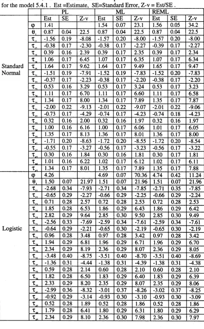
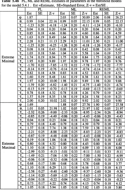
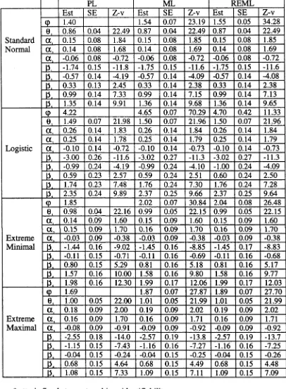
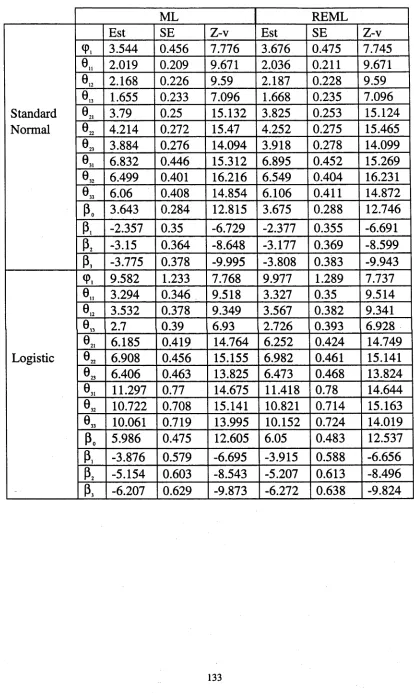
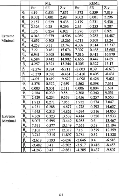
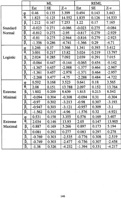
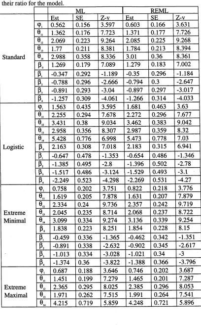
Chapter 10 demonstrates a simulation study. For each of the threshold

models given in chapter 5, observations are generated under the three

different random component structures; one component, two components and

AR(1). In the one component structure, the random components are

distributed as normal with zero mean and constant variance. Two random

components vectors are assumed to be independent in the two components

structure. The random components are given a first order autoregressive

process in the AR(1) structure. In this chapter, the simulation results are

provided for both ML and REML methods for all combinations of the

parameters.

Chapter 11 discusses the results for the threshold models. Some

results in matrix algebra are provided in appendix A. Appendix B gives

the data sets that are used in applications of the different random components

threshold models in different chapters. Appendix C gives some the programs

that have been written in DYALOG APL version 7.1 to carry out the

computations of the thesis.

1.4 COMMENTS

1 In chapter 5-9, some of the ordinal data sets are commenced at zero

and some at one. Without loss of generality, the threshold models and

estimation results are given for ordinal data sets that coding begins at zero.

2 During preparation of this thesis four papers have been submitted for

different journals. Two of them have been accepted for publication and

other two are in process. Chapters 5 and 6 are an extension of the accepted

papers.

CHAPTER TWO

LITERATURE REVIEW OF COMPONENTS OF

VARIANCE IN CONTINUOUS MODELS

2.1 INTRODUCTION

Statisticians have introduced two important types of models to study the

dependence of a response variable upon explanatory or regression variables.

A traditional, useful and more applied type of modelling is called a fixed

effect model, which focuses on the variation that is caused by factors that are

in the sample. This model has been extensively investigated since Legendre

(1806). The other type of modelling is known as a mixed model. It also has

a long history, but has received special interest only in the last few decades.

The neglect was partly due to the heavy computational burden in the

estimation methods. Developments in computing hardware, software and

estimation methods have brought much attention to the mixed model.

The aim of this chapter is to give a brief discussion of the

development of variance components, for detailed review of this issue please

see Searle, Casella and McCullagh (1992). The following sections attempt to

outline some of the basic work on the variance component theory that is

fundamental to the development of Generalized Linear Mixed Model

(GLMM) approaches. The relevant works are; best linear unbiased predictor

(BLUP), maximum likelihood and residual maximum likelihood methods.

2.2 MIXED MODELS

Most of the Statistical models that are applied to data sets can be

considered as special cases of a general mixed model

2.2.1 y=Xß+Zu+e

where y is a nxl vector of observations, ß is a pxl vector of unknown

regression parameters with known nxp design matrix X, incidence matrix Z

corresponding to random component u . Moreover, u can be partitioned

into q subvectors

2.2.2 u = [u;,u;,...,u;r

where iij is a VjXl vector of random components with incidence matrix

Zj . The matrix Z is partitioned conformably to the partition of u as

Z = [Z1,Z 2,...Z J . Furthermore, it is assumed that

2.2.3 = 0, for j=l,2,...q, and E(e) = 0

E(y) = Xß, and E(ylu) = Zß + Zu = Xß + £ Z u

j - i J J

VartUj) = a ]A /p ), for j=l,2,3...q, C o v ^ u ,) = a ] Z iX i

Cov(u j,uj,) = 0, for j * j ' = l,2,3...q, Cov(uj,e) = 0,

Var(e) = o 2D, Var(y) = V = a 2D + Z(var(u))Z' = V ,

where

p

(p

1

,p

2

,...ps)',

blocks being matrices g] A ^ p ), for j=l,2,3...,q.

Sometimes, matrix var(u) is given in terms of ratio of a; to a \ i.e., if

a] / a

2.2.4 A =

<P,A,(P)

<PA(P)

<P,A,(p)

From 2.2.3 and 2.2.4, we have

2.2.5 Var(y) = g2(D + ZAZ) = g2I , D + ZAZ = Z .

The g2 and elements in the vectors p and cp are called variance

components. The resulting models are known as variance component models.

The appearance of such models has a similar history to the fixed

effect model that Legendre (1806) and Gauss (1809) discussed for the first

time in books on astronomical problems. Airy (1861) wrote down the model

of 2.2.1 as

a

2.2.5 y^ = |i + u k +e , for i=l,2,3,...a and k=l,2,3...n , n = £ n, with

‘ i=l '

2.2.6 V ar(uJ = Gu, V ar(eJ = G 2, Var(y J = Gu + g2 .

Chauvenet (1863) applied model 2.2.1 without writing down model

equations. It is not well known that astronomers, long before statisticians,

also formulated variance components models (Scheffe 1956).

2.3 ANOVA

Sir Ronald Fisher (1918) introduced the terms "Variance" and "Analysis of

Variance" (ANOVA). He also (1925) proposed equations that later became

the central idea for estimating variance components.

Tippett (1931) proposed ANOVA methods for one-way and two-way

classification. Sampling design was introduced by Yates and Zacopanay

(1935). Other important works are Daniels (1939), Winsor and Clark (1940)

on the ANOVA methods. Ganguli (1941) extended Winsor and Clark's

discussion to the multi-way and nested classification. Crump (1946, 1947)

used ANOVA methods to estimate variance components in random effect

models for balanced data. He derived the distributional properties of

estimated variance components by applying the following criteria for

balanced data.

If components in the random effect models follow the normal

distribution, then any mean square in an ANOVA table, say ms, with f

degree of freedom are distributed as

2.3.1 E (m s)f1 x].

In addition, for any estimated variance components, say

2.3.2 G2 = am s,+...+ am st ,1 1 k k 7

where ms. (j=l,2,...k) is a mean square based on f degree of freedom, has

sampling variance,

2.3.3 V ar(a2) = 2 a;[E(ms1)]2 E'+...+2a;[E(msk)]2 f;1.

Daniels (1939) suggested to replace f by f +2 in 2.3.3.

Eisenhart (1947) gave a comprehensive description of two types of

models, the fixed effect models (type I) and random effect models (type II),

see Scheffe (1956), Anderson (1978), Searle (1988) and Searle, McCullagh

and Casella (1992). Crump (1951) gave maximum likelihood estimators of

variance components by replacing negative values with zero in the ANOVA

methods for the type II models of Eisenhart.

The major work for the unbalanced models was done by Henderson

(1953). He introduced three types of methods for estimating variance

components. In method I, he applied ANOVA methods to estimate variance

components. He adjusted for fixed effects in a mixed model, then he

employed ANOVA methods for the adjusted model, in the method II.

Method III uses reduction in sum of squares. This method is called the

fitting constants method. Herbach (1959) used the maximum likelihood

principle to estimate variance components. Thompson (1962) proposed the

restricted (residual) maximum likelihood method. Searle (1956) introduced

variance components in terms of matrix format. Mahamumula (1963)

extended Searle's (1956) work to the unbalanced three-way classification.

There are also some other methods of dealing with variance

components. For example, the Bayesian method, was introduced by Hill

(1965, 1967) for balanced models. The most important work using Bayesian

methods is Gnot and Kleffe (1983) for unbalanced models. Rao (1971a,

1971b, 1979) introduced a general method called MINQUE (minimum norm

quadratic unbiased estimation) method into the variance components

literature.

Maximum likelihood (ML) and residual maximum likelihood

(REML) are two frequently used methods with variance components.

We will go through the development of one of the important

approaches that is very useful for deriving ML and REML estimates of

variance components. The approach is Best Linear Unbiased Predictor

(BLUP). It might have been mentioned that the ML and REML approaches to

variance components would be taken in sections 2.5-2 1.

2.4 BEST LINEAR UNBIASED PREDICTION

(BLUP)

In a series papers Henderson (1948, 1949, 1959, 1963, 1973, 1975)

developed the BLUP method. It became a powerful and widely used

procedure in animal breeding to evaluate genetic trends of animals for traits

measured not only on the continuous scale, but also on a categorical scale.

Robinson (1990) argued that the term BLUP was applied by Goldberger

(1962) for first time and Henderson started using the acronym BLUP in

(1973). However, it was Henderson in (1948, 1949) who discussed the

deficiency of classical least square methods. Henderson et al (1959)

proposed a solution to this problem by using a discussion given in Henderson

(1950). Henderson introduced a predicted value of u as a linear function of

y. He continued discussion on the prediction by including predicting or

estimating a linear function of fixed effects and random effects in 1973. He

proposed the BLUP method to predict and estimate random effects and fixed

effects in cases where the assumption of random sampling is seldom valid.

Suppose that we have a set of observations say y, where y is defined in the model 2.2. The matrix Z is known and random effect u has the same distribution structure as the model 2.2. Then the BLUP method is designed to handle the prediction of u j when second moments of the joint distribution of y and u j are known. Henderson (1963) in an attempt to predict ui , used a prediction of a linear combination of random effect u j and fixed effect ß. Let us define an unobservable random vector £ , which

is jointly distributed with y as

2.4.1 C)i = Bjß + Uj, forj= l,2,...q.

Both means of ^ and y are given in terms of the unknown parameter vector ß.

Theorem 2.4.1:

1 E ( ^ ) = a jS forj= l,2,...,q where a ^ B J J 2 Var(CJ) = a 1 29 JA j

3 C ovC ^C ;,) = 0 ,fo rj* j'= l,2 ,...,q 4 C o v ( ^ ,e ') = 0 fo rj= l,2 ,...,q

5 C ov(y,£') = a 2 (pjA JZ ' = C r for j= l,2,...,q.

Proof:

1 E (^j) = E(Bjß + u j)=Bjß + E (u j)= B jß= a j? using E (u J) = 0 . 2 Since is a fixed value, we have V ar(B ^) = 0 and

Cov(Bjß, Uj) = 0 . Therefore,

Var(CJ) = Var(BJ3 + u J) = Var( u J) = a 29 JA j.

3 C o v ^ .C ,) = Cov(Biß ,(B ,ß )/) + Cov(BJß ,u ;) + Cov(u j,(Bj ß)') + Cov(ur u'y) = 0 + 0 + 0 + Cov(Uj, u ' ) = CovCUj, u ' ),

since u i and u ' are independent, therefore

Cov(£Jt£ ' ) = Cov(uJ, u ') = 0.

4 Cov(£.,e') = Cov(Bjß,e/) + Cov(uj,e') = CovCu^e')

the Uj and e are independent, thus

Cov(£.,e') = Cov(uj,e/) = 0.

5 Cov(y,£') = Cov(Xß, (B J(ß)') + Cov(Xß, u ') + Cov(Zu, (B ß)') +

Cov(Zu, u ') + Cov(e, (B ß)') + Cov(e, u')

= 0 + G + 0 + 0 + 0 + Cov(Zu,u') = CovftX^ZjUj),!!')

from independence of u} and u y for j^j'=l,2,...,q wehave

Cov(y,^') = C o v C Z ^u ;) = c r c p ^ Z ; ,

by this the proof of the theorem 2.4.1 is completed.

Following Henderson (1963), if £jh is the h* element of the vector

then £jh, the predicted value of ^Jh, should be linear function of y, i.e.,

2.4.2 £jh = A'hy + Vjh, where A» and Vjh are vector and scalar respectively.

The unbiasedness and minimum mean square in the class of linear prediction

are two otiacx properties of the BLUP method. So

2.4.3 E( ^Jh) =E(£jh) i.e, £jh is an unbiased predictor for ^Jh and

2.4.4 E( £Jh -£jh )2 should be mininimized.

From theorem 2.4.1 and 2.4.3, 2.4.4, we have,

2.4.5 E (£jh)=A'hE(y) + V jh _ A 'X ß + Vjfc=E (^jh)= B ;ß

where the B'h is the h* row of the matrix B .

For Vjh not dependent on the ß, the relation 2.4.5 holds if

2.4.6 A 'X ß = B'hß, which implies V h=0.

For C jh = C ov(y,£jh), the problem of predicting £jh reduces to a minimization of a function say F(Ajh) with respect to the Ajh with a constraint G(Ajh)=0 given in 2.4.6. Therefore, the problem is

2.4.7 Minimise F(Ajh)= [A ;iA jh + v a r(^ h) - 2 A ; C J subject to: A'hX = B'h

The problem 2.4.7 can be solved by introducing a vector 2 \ of Lagrange multipliers. So we find the derivatives of

2.4.8 F0( A ^ M A ; Z A , + v a r ( O - 2 A ; C >+2 ( A ; x - B ; ) H

Differentiating 2.4.8 with respect to Ajh and X yields

2.4.9 XAjh- C Jh+ X * = 0

2.4.10 X'Ajh = Bjh or in the matrix format these two equations is given by

2.4.11 "X X"

r \ i r c j

1 >< o I >> i___ w i

A generalized inverse of the matrix of coefficients 2.4.11 is given by using Searle (1982) (p-261-262) as

2.4.12 z _l

0 0

0 + ( - X '

Therefore, using 2.4.9 , the Ajh is given by,

2.4.13 Ajh=Z~‘ Cjh + Z" X(X' Z" X)(Bjh - X' Z" Cjh).

Replacing 2.4.13 into the equation 2.4.2 yields,

2.4.14 ^ = [ r c jh+ r x ( X ' r x ) ( B jh- x ' r c Jh)]'y =B»(X'Z" X)X'

r

r

We may replace Xß = X ( X ' Z 1 X)X'Z'1 y in the equation 2.4.14 and obtain,

2.4.15 ; ll = B'Jlß + c ; z - ,( y - x ß ) = d >.

A

where ß is the Aitken's generalized least square (GLS) estimator of the ß. Then the BLUP of ujh is obtained by taking B jh equal to zero in 2.4.15

2.4.16 ü jh= c ; z " ( y - x ß ) .

Equation 2.4.16 gives

2.4.17 üJ = Cj r ( y - x ß ) , giving ü = C r ( y - X ß ) ,

2.4.18 £ = B ß + C , Z " ( y - X ß ) , giving, \ = Bß + C Z " ( y - X ß ) .

Henderson (1963) developed equation 2.4.17, and he also (1973) introduced equation 2.4.18 to predict a linear combination of fixed effect, say ß, and random effect u.

2.4.1 SOME CHARACTERISTICS OF THE BLUP

The BLUP method also carries some other properties as follows.

1 Henderson (1963) showed that under certain assumptions (including

normality) the BLUP estimators of u maximise the probability of correct

ranking of u. An extension of this is given by Portnoy (1982).

2 The conditional expected value of u for given y is the BLUP

estimate of u under the normality assumptions. See Henderson (1963).

3 In the class of linear predictors, BLUP estimators maximise the

correlation between the predictor Ü, and predictant u.

4 Henderson (1973) extended the BLUP to predict k'ß + m'ii by

k'ß + m 'ü, where ß and ü are BLUP estimators of ß and u.

2.4.2

HENDERSON MIXED MODELS

EQUATIONS (MME)

It is clear that the BLUP method can hold if the covariance between

observable random variable y with non observable random variable u is

known, but equation 2.4.17 involves the inverse of the variance-covariance

matrix of y which is potentially large in many applications.

An alternative way to get BLUP estimators was introduced by

Henderson (1950). The approach estimates ß and predicts u simultaneously.

These are values of ß and u that maximise the logarithm of the joint

density function of y and u , denoted by 1. The function 1 can be written as

2.4.2.1 1 = 1, 12 where

2.4.2.2 1, = -(1 / 2)[const.+nlnö2 + |D| + a~2( y - X ß - Z u ) 'D 'l( y - X ß - Z u ) ]

2.4.2.3 1, = -(1 / 2)[const.+vlna'2 + ln|A| + g 2uA u] ,

where v = Y?.v. and v is the dimension of random vector u, for

j=l,2,...q. Equating to zero the derivatives of 2.4.2.1 with respect to the ß

and u yields equations

X ' D y

Z'D y

These are called the Mixed Models Equations (MME). Let V be the matrix

coefficient in 2.4.2.4 and non-singular. Then using lemma 1 in appendix A,

it can be easily proved that

2.4.2.4 X'D X X'D Z ß

Z'D X Z'D Z + A Ü

r v v 1-1 o o I

2 .4 .2 .5 V 1 = 11 12 = B = + V ' V

L 12 22 _ _° v i . _y-> V ' L Y 22 T 12 J

where

2.4.2.6 G = [Vu - V12 V i V 'y , and B =

g

[

i

-w.:]

. T

The submatrices in the matrix V are

2.4.2.7 Vu = X'D ‘X, V12 = X'D Z, and V22 = Z'D Z + A " .

The corresponding submatrices in the matrix B are,

2.4.2.8 Bu = [XTTX - X T TZ T ’Z 'D -'X r1 =(X'Z-‘X)-1,

2.4.2 9 B 2 = T* + T Z'D XB X'D ZT , and B 2 = -B X'D ZT .

where T* = ( A 1+ Z 'D Z )".

From the above, ß and ü are

2.4.2.10 ß = [B ,X' + Bl2Z ']D ‘y

= B X'[D 1 - D ‘T Z'D ]y , by using equations in 2.4.2.9 =B llX'Z y = (X 'X -'X jX T -y and

2.4.2.11 ü = [B',X' + B;;Z']D y

= B :1X '( [ I - D Z T Z '] + T Z ') D y , by using equation in 2.4.2.9 = B X X y + T Z D y = - T Z D X (X 'D X jX 'X y + T Z D y = T Z 'D ‘ [y - Xß] = A Z 'X '1 [y - X ß ].

«V / s

Henderson (1959) proved that ß in the 2.4.2.10 is identical to the GLS ß. He (1963) also proved that predicted value given in 2.4.2.11 is identical to those in 2.4.17.

2.4.3

DISTRIBUTIONAL PROPERTIES OF ü

AND ß

The proceeding developments are based on the theorem 2 of appendix A.

Theorem 2.4.3.1 :

1 V ar(k 'ß ) = o 2k 'B nk , 2 C o v (k 'ß ,ü ') = 0 ,

3 C o v (k 'ß ,u ') = -c T k 'B l2, 4 C o v ( k 'ß ,ü '- u ') = a :k 'B l2, 5 Var(ü) = G2( A - B J ,

6 C ov (u ,u ') = V ar(u), 7 V a r ( u - u ) = g'B ^,

8 V ar(k 'ß + m 'ü - k 'ß + m 'u ) = G2[k', m']rB„n B l k"

B :l

12

B ,. m

9 Var((G/,u ,))/ = g2

A - B ;2 A - B 22‘

A - B:, A

Proof:

1 Var(ß) = [B„X' + B Z ]D G [D + Z'AZ]D [BnX' + B Z']'

= B X'[I - D ZT Z']D G [D + Z AZ]D [I - ZT Z D 1 ]XB

= B X'[D - D ZT Z D ]g [D + Z AZ][D 1 - D ZT Z'D ]XB„

= G B ,X 'I I I XB ,=

o Bu.

Thus, Var(k'ß) = G2k'B nk.

2 Cov(ß,ü') =

= B X [I - D ZT Z']D G [D + Z'AZ]D 1 ([I - ZT Z D ]XBi: + ZT )

= G BnX'([D - D ZT Z D ]XB +ZT )

= g2(BuX 'I XBi; +B X'D ZT ) = G (-B X D ZT + B „X D ZT )

=0.

Therefore, CovCk'j^u'm) =0.

3 Cov(ß,u') = BnX '[D 1- D 'ZT’Z'D 'JcovCy,^)

= B X [D 1 - D 'Z T ’Z 'D ' ]cov(Xß + Zu + e,u')

= G B X [D - D ZT Z D ]ZA

= G2 B .X 'I 'ZA, and using

X T Z =

= G2 B. X'D ZT A A=- g2B 2, so Cov(k'ß,u') = -G 2k'B l2.

4 Cov(ß,ü, - u ') = Qcov(ß,ü,)P/ - B llX'[D-1-D -Z T 'Z 'D 'Jco v C y ^')

=0-- G2B12= o B12, giving C o v (k 'ß ,ü '-u ') = c rk 'B l2

where Q and P are known matrices.

5 Var(ü) = [B 'X ' + Br Z']D G2[D + Z'AZ]D [B 'X ' + B22Z ']'

= G (B; X [D 1 - D ZT Z'D ' ] + T Z D 1 )Z([D 1 - D ZT Z D ]XB + D ZT ) = g: (b;:x'z-‘ +t z'd ) i ( i x b + d z t )

= G (B; X I XB + T Z'D XB : + B 'X D 'Z T ‘ + T Z D ZD ZT ) = a (-B ;X 'D ZT + T Z 'D XB ; + B ; X'D ZT + T Z'D ZD ZT ) = g (T Z 'D X B ; + T Z 'D ZD ZT ) = g (T - B r + A - T )

= a : ( A - B „ )

Thus, Var(u) = G2( A - B J .

6 Cov(ü, u')=[B;2X ' + B;:Z']D 1 cov(y, u ')

= a 2 (B 'X '[D - D ZT Z D ] + T Z 'D )ZA =g2(b;x'z-'z a +t‘Z 'd -'z a)

=g2(b;;x,z"z a +a - t‘)

= g (B;;X D ZT + A - T )

= g2(T ‘ — B ;, + A - T ‘) = g:( A - B ;:) = V ar(u) therefore, Cov(u, u ') = V ar(u ).

7 Var(ü - u) = Var([B;:X' + B^Z']D y - u)=

[B;2X ' + B:;Z '][D + Z A Z '][B 'X ' + B ::Z ']' + Var(u) - 2[B;:X ' + B =Z']Cov(y, u ') = g (A - B^ + A - 2 ( A - B 22)) = g2B 22

therefore, V a r ( ü - u ) = o B,,.

8 V ar(k'ß + m 'ü - k 'ß + m 'u)

= k'V ar(ß)k + m 'V ar(ü)m + k 'V ar(ß)k + m 'V ar(u)m + 2k'Cov(ß, ü ')m - 2k'Cov(ß, ß ')k + 2k'Cov(ß, u ')m - 2m 'Cov(ü, ß ')k - 2m'Cov(ü, u ')m + 2k'Cov(ß, u')m = G ( k 'B uk + 2 k 'B l2m + in 'B 22m)

= G2 [k', m']

I X

1

A

12

B , . m

Result 9 follows from 5 and 6.

2.4.4

NORMALITY

Application of the BLUP method with all the properties given in the previous section can hold without assuming normality for the joint distribution of the u and y. Nevertheless, that assumption contains certain properties that are based on properties of the normal distribution given in theorem 2 of appendix A.

Theorem 2.4.4.1:

1 The ß and G are identical to the corresponding maximum likelihood estimators derived under normal theory assumptions and given variance-covariance matrix of y denoted by GJ Z .

2 E(u|u) =G

3 Var(u|G) = V ar(u)-V ar(G ).

The proof is given in Searle et al (1992) (page 273).

Thompson (1979) argued that the Henderson (1975) is hard to understand and made some modification to the Henderson approach. A generalization of the Henderson BLUP approach is Harville (1976). Goldberger (1962), in an attempt to predict a single drawing of the regressand given the vector of regressors noted that the prediction disturbance is correlated with the sample disturbance. He used the BLUP

method to give a prediction. Bulmer (1980) proposed a two stage BLUP

method. Gianola and Goffinet (1982) showed that the two stage method of

Bulmer is equivalent to Henderson's BLUP. Robinson (1990) has reviewed

BLUP. Searle, Casella and McCullagh (1992) have discussed BLUP

methods in more detail.

The developments in these sections is concerned with estimation and

prediction assuming that the variance components are known. Perhaps, in

practice, we may encounter a problem in which neither first nor second

moments are known. Of course we never really know parameter values, but

we may have good prior estimates of them.

There are three methods under Henderson's name to estimate variance

components. These were the most frequently used methods up to 1970.

Subsequently the estimation of components of variance relied more heavily

on the maximum likelihood and residual maximum likelihood methods.

Henderson (1975) showed that estimates and predictions are biased by

substituting estimated values of variance covariances into selection models.

Kackar and Harville (1981) proved that two-stage method (first estimate

variance components, then use these to estimate and predict fixed parameters

and random components) gives unbiased estimators and predictors provided

the distribution of the data vector is symmetric about its expected value and

provided the variance component estimators are translation invariant and are

even functions of the data vector. They showed that the ML, REML and

ANOVA estimators involve those properties. They also (1984) argued that

by replacing true values of variance components with estimates, the

estimators are BLUP but the mean squared errors increase in size. They

proposed a general approximation to the mean squared errors. Harville

(1985) extended this approximation generally.

2.5 MAXIMUM LIKELIHOOD (ML)

The difficulty with the establishedTnethods discussed in the previous

section was partly the impetus for a continued search into other methods.

The most frequently applied method to estimate the variance components is

maximum likelihood (ML). This is partly because the ML method has a

number of well-known features, some of which are mentioned by Harville

(1977). The ML method requires that a distribution be attributed to the

random component in a mixed model. It is often confined to the normal

distribution on continuous data. The general mixed model we consider is the

same as that given in the section 2.2 with the following additional properties.

For observation vector y from a mixed model given in the section

2.2, the log-likelihood function is given by,

2.5.1 1 = -1 / 2[cont.+ ln|V| + (y - X ß / V 1 (y - X ß)].

Maximum likelihood estimates for the

ß, cf, p,

maximise the log-likelihood 1. Differentiation of the 1 with respect to

ß, a 2,

o '

p t

2.5.2 a i/3 ß = a-2[X'V-1(y -X ß )],

2.5.3 01/aa2 =-(l/2)[tr(V-ia v / a a 2) - ( y - X ß ) ' y ,a v / a a 2V'1(y-Xß)],

2.5.4

d \ / d a ] = -(1 / 2)[tr(V"ZjAjZ;) - (y - X ß ) ' V lZ JA Z ' V ( y - X ß)],

2.5.5

öl / öp, = -(1 / 2)[tr(V ,ZÖA / öp Z ') - (y - Zß/V 'ZÖ A / öp Z 'V 1 (y - Xß)].

Equating 2.5.2, 2.5.3, 2.5.4, and 2.5.5 to zero yields the ML estimators.

However, the resulting equations for 2.5.3, 2.5.4, and 2.5.5 are nonlinear and

have to be solved numerically for a general variance-covariance matrix V.

Fisher (1925) introduced the ML method. Crump (1949, 1951) and

Herbach (1959) give an important discussion of this method. The

computational and some other problems were the reasons for this neglect of

the ML method until 1967. Hartley and Rao (1967) proposed a solution to

some of those problems and brought greater attention to this important

method.

Hartley and Rao (1967) introduced simultaneous estimation equations

for variance components and obtained ML estimates by some numerical

techniques. They formulated variance-covariance matrix of y in terms cpjS

the ratios of a] s to the a . Their likelihood or log of likelihood function is

based on the matrix H given by

2.5.6 V = a 2H = a 2 [I + ZAZ']

where the A is a block diagonal matrix of blocks as the jth diagonal

block and I is an identity matrix of the corresponding dimension. Using

2.5.6 in the derivatives 2.5.2, 2.5.3 and 2.5.4 gives

2.5.7 X'H"‘y = X'H~‘Xß,

2.5.8 a 2n=(y - Xß)'H"‘(y - Xß)

2.5.9 = a 2(y " Xß)'H"1Z JZ'H"1(y - X ß ).

The derivative with respect to p is zero since 2.5.6 does not depend on the

parameter p. The ML estimators of ß and a 2 can be easily derived from

2.5.7 and 2.5.8. The ML estimation equation of cpj is given by

2.5.10 «9^=0.

It can be solved by

2.5.11 = (pjo- f(<p„,)f'«p,.)>forj=l,2,3,...q.

Hartley and Rao (1967) also introduced an alternative estimation equation by

applying the joint likelihood of y and for some j and then obtaining

likelihood L as the marginal of y by integrating over ui.

The implementation of the Hartley and Rao (1967) approach involves

taking the inverse of the H matrix that has a dimension as large as the

number of observations. Hemmerle and Hartley (1973) introduced a W

transformation to reduce the computational problem in yielding ML

estimates for mixed ANOVA models. They obtained estimates of ß and cr

for given cp^ and then used those to perform a numerical solution for cpr

Jennrich and Sampson (1976) applied Newton-Raphson and score numerical

methods to obtain simultaneous estimates of fixed effects and variance

components in the mixed ANOVA models. An efficient Cholesky type

algorithm to perform transformation W was developed in Hemmerle and

Lorens (1976).

2.5.1 ASYMPTOTIC VARIANCE-COVARIANCE

One of the advantages that the ML method carries is the ability to obtain

large-sample asymptotic variance-covariance of the ML estimators. The

asymptotic variance-covariance matrix for the ML estimators is the inverse

of the information matrix. The information matrix is given by

ppr

L

K

L

K

C

K

K

K K

where the elements are second order derivatives of 1 with respect to

appropriate parameters.

Hartley and Rao (1967) derived the limiting properties of the ML

estimators of ß and ratio's cpj s as both number of individuals (n) and

number of random effects (v.) become infinitely large (j=l,2,...q)

simultaneously in such a way that the number of observations falling into any

particular level of any random effect stays below some universal constant.

Searle (1970) extended Hartley and Rao (1967) by including more variance

component parameters. Miller (1973) argued that the latter restriction greatly

limits the applicability of the Hartley and Rao results. He (1977) generalised

Hartley and Rao (1967) further.

2.6 RESIDUAL MAXIMUM LIKELIHOOD

(REML)

One criticism to the ML method of estimating variance components is

that it does not take account of the reduction in degrees of freedom due to

estimation of fixed effects in estimating variance components. Residual

maximum likelihood (REML) method was established to cover this

weakness of the ML method. In some balanced models, REML estimators

are identical to those given by the ANOVA with well known properties of

unbiasedness and minimum variances. As it is often defined, the REML

method derives estimated variance components from the following log-

likelihood function, 1',

2.6.1 1' = -1 / 2[cont.+(n - p) In a 2 + ln|KZK| + c r y K(KZK)Ky].

where K = D l - D X(X'D X) X'D 1 is a symmetric matrix and

X'KX = 0 implies KX = 0.

Differentiating 2.6.1 with respect to a 2, qv, ps yields

2.6.2 d V / d a 2 = - l / 2 [ a -2(n -p )-a V K (K 5 ;K )-K y ],

2.6.3 31'/3(pj =

-1 / 2[tr((KIK)- K(0Z / dq> J )K) - a " 2y'K(K£K)~ K (01 / 3cp J )K(KIK)- Ky]

2.6.4 3 1 '/3p, =

= -1 / 2[tr((KZK)- K(3Z / 3p, )K) - cryK (K X K )- K(dZ / 0p, )K(K2K)' Ky]

Equating 2.6.2-2.6.4 to zero yields REML estimation equations of a 2, cpj9 ps

which have to be solved by some numerical techniques. The asymptotic

variance-covariance of the REML estimators of g2, (pj? ps is inverse of the

information matrix I DCMI, viz.,REML 7 7

' V " o 'ip o*p

l' W 1'W>

• C

-where elements inside the information matrix are second derivatives of 1'

with respect to component parameters.

2.6.5 I REML ~ E

1'

oV

The REML method dated back to Anderson and Bancroft (1952). In an attempt to derive a non-negative value of variance components, Thompson (1962) used the REML method. Patterson and Thompson (1971) described this method in the Hartley and Rao's (1967) way for simple mixed

models, a generalization of Patterson and Thompson’s (1971) was derived by Corbiel and Searle (1976).

2.7 FROM BLUP TO ML AND REML

Implementation of the ML and REML methods in previous sections involve evaluating first and second order derivatives of the corresponding log- likelihood functions to obtain ML and REML estimators and their approximate variance-covariance matrices. However, except for some special mixed models, computational problems arise in application of the ML and REML methods. Harville (1977) gave some solution to the computational problems of the ML and REML methods by introducing a link between section 2.4 (BLUP) and sections 2.5, 2.6. He used BLUP equations to set up iterative procedures in calculating ML and REML estimators of variance components and their asymptotic variance-covariance matrices for ANOVA mixed model. He stated that the establishment of the numerical methods might be improved by making the log-likelihood function more quadratic. Harville (1977) also argued that the REML method is a method that is marginally sufficient for variance components in the sense given by Sprott (1975). Fellner (1986, 1987) discussed Harville's (1977) method for some special models. The method was reviewed in more detail by Thompson (1981). The derivation of the link between BLUP, ML and REML will be discussed further in chapter 4.

2.8 NONLINEAR MODELS

There are also some problems concerned with a continuous random

variable y related to fixed and random effects by a respecified nonlinear

function f. Sheiner and Beal (1985) discussed a least square approach to the

non linear random effect models. They have taken a linearization of the

nonlinear function f(.) about 0. A Bayesian approach was proposed on

random models by Racine-Poon (1985). Lindstrom and Bates (1990) have

derived ML and REML estimates of variance components by linearizing f(.)

about the current estimated values of random effects. Vonesh and Carter

(1992) have also linearized about current estimated values of random effects,

and used a four stage generalized least square. Gumpertz and Pantula (1992)

have employed the linearization and discussed ML and REML methods. An

extension of Sheiner and Beal (1985) is given in Solomon and Cox (1992).

CHAPTER THREE

LITERATURE REVIEW OF COMPONENT

VARIANCE IN DISCRETE RESPONSE

VARIABLES

3.1 INTRODUCTION

The preceding chapter has addressed various forms of variance

component estimation in continuous random variables, topics that have been

extensively investigated. Success in developing estimation and inference

techniques is partly due to the existence of a well known normal distribution

for these families of random variables. Roughly speaking, in the most cases,

continuous response data is analysed by relating the means of various normal

distributions to underlying factors, and an idea behind the estimating of

variance components is to obtain more reliable inferences about means.

Although estimation and inference techniques in discrete response

variables are not comparable with continuous cases, the analysis of discrete

data has a long history dating back to 1662. In 1662, John Graunt collected

the frequencies of death from several causes, as well as frequencies of birth

and he concluded that more male than female children were bom.

Estimation and inference techniques are not easy to apply to

regression problems with discrete response variables. Also the range of

analysis associated with discrete data is very wide. For example, in a cross­

classification table, one may focus on the estimation and inferences

techniques about association between row and columns, whereas others may

wish to estimate and make inference about odds ratios or relative risk.

For the many problems, the focus is on the probability of a certain

event (P). The estimation and inference of P becomes more difficult when it

is modelled in terms of some covariates. Yet more problems arise when

models on the P involve not only covariates but also terms corresponding to

random components.

In this chapter, we review the estimation and inferences techniques in

discrete response variables.

3.2 WEIGHTED LEAST SQUARE (WLS)

While log-linear models were used for estimation and inferences in

cross-classifications, several alternative approaches were also applied to this

class of response variable. Kullback and Ku (1968) and Ireland et al (1969)

investigated the procedure for minimum discrimination information

estimation to estimate and make inference about multinomial probabilities.

Neyman (1949) derived best asymptotic normal (BAN) estimates of cell

probabilities by minimising the usual Pearson chi-square statistic (X’). He

introduced a modified chi-square by replacing the expected value in the

dominator of the usual chi-square with the observed value. He also

described an alternative way to minimise the modified chi-square (X*) by

imposing constraint functions on cell probabilities. He used first order

approximation for constraint functions and proved that the resultant estimates

are BAN. This last approach of the problem of minimising X2N has potential

as a theoretical base for some later approaches.

Berkson (1968) applied constraints to minimise logit X2 to the

problem of Grizzle (1961). Yet another important application of constraints

on cell probabilities is Grizzle et al (1969). They introduced a general class

of weighted least squares (WLS) estimate and inference approach to analyse

categorical response variables. The approach has the advantage that one can

utilise the same algorithm as that used for the analysis of the linear models

with normally distributed errors, and it permits great latitude in choosing

models. It also unifies some previous approaches into one framework.

Briefly, let i(i=l,2,3,...I) refer to factors and j(j=l,2,3,...r) indicates the jth

category, then n.. denotes frequency of the ith factor and jth category in

cross-classification of factors with categories. Assume that the vector

n' = (niI,n i2,n i3,...,n ir) follows the multinomial distribution with components

of n. = X Jr=1n.. and n' = (nil,ni2,ni3,...,njr). Let P, be the observed value for

, , / estimated

the n. and P = [P,P2,P3,...,P j . Thej(vanance-covariance matrix of P is a

block diagonal matrix with blocks

3.2.1 V(P() = m‘[Dp( -P.P.'J

where Dp is a diagonal matrix of elements vector P(. For any function

F=Xß of the P that has partial derivatives up to second degree with respect

to p, the sample variance-covariance matrix of F, by applying 5 method, is

r)F

3.2.2 S=HV(P)H’ where H = — .

8P

/V

The WLS method tries to find an estimator for ß say ß that minimises the

quadratic form

3.2.4 ( F - ß ) 'S - '( F - ß ) .

Koch and Reinfurt (1971) extended WLS to split-plot experiments

and Koch et al (1972) applied the WLS to incomplete response data. Two

approaches to estimation and inference for ordered categorical response by

using WLS were given by Williams and Grizzle (1972). Koch et al (1977)

generalised the paper by Koch and Reinfurt (1971) to repeated measurement.

In studying longitudinal clinical trials with missing responses, Standish et al

(1978) gave some discussion on the WLS approach. Stanek III and Diehl

(1988) applied the WLS method to develop a growth curve model for binary

response. In developing estimation and inference for longitudinal

polytomous response, Miller et al (1993) have discussed the connection

between WLS and GEE and have suggested the need for further study.

Application of the WLS approach to repeated categorical measurements with

outcomes subject to non-response is in Lipsitz et al (1994).

3.3 ASSOCIATION MODELS

As soon as the data is arranged in a table, the measure of association

is one of the important questions that have been addressed in the statistical

literature. Kendall et al (1961) and Edwards (1963) defined various

functions for the measure of association. While the association is between

two or more variables, it is required to integrate a bivariate distribution in

simple cases or multivariate in some applications.

Plackett (1965) and Gumbel (1960, 1961) introduced Plackett and

exponential bivariate distributions respectively. These families of

distributions have been used occasionally when the approach needs to

calculate integrals of bivariate distributions.

Bhapker and Koch (1968) investigated interaction in

multidimensional cross-classifications for various possible combination

structures. Symmetry and marginal symmetry in a multidimensional table

were studied by minimum discrimination estimation procedure in Ireland et

al (1969). Ashford and Sowden (1970) presented an extension of the probit

model and used correlation in bivariate normal underlying distribution as an

association between bivariate discrete responses. A logistic model that

allows for the inclusion of an associated occurrence between two responses

is in Mantel and Brown (1973).

Goodman (1979) introduced different association models for

contingency tables with ordered categories. He modelled association in

terms of the odds-ratios in 2x2 subtables built from adjacent rows and

adjacent columns. Plackett's class of bivariate distributions was used for

analysing the pattern of association in cross-classifications with ordered

categories in Wahrendorf (1980). Goodman (1981) generalised the

association models in Goodman (1979). He compared the association model

approach with the canonical correlation method for estimating and testing in

cross-classification with ordered categories. Association models were used

to derive an estimate for the correlation parameter in the underlying bivariate

normal distribution in Goodman (1981). He showed the association models

approach more closely the bivariate normal than Plackett's does.

A test was proposed for dependence in multivariate probit models by

Kiefer (1982). Dale (1984) compared local and global association in cross­

classification with ordered categories. The relationship between the latent

class and canonical models as two approaches for cross-classification with

ordered categories, was studied by Gilula (1984).

Anderson and Pemberton (1985) extended Pearson (1904) and Tallis

(1962) to multivariate responses and derived estimates of the cut-points from

the one-way marginal distribution. They obtained an estimate of the

correlation matrix by polychoric correlation coefficients from cross­

classification. In 1985 and 1991, Goodman gave two comprehensive lectures

for analysing cross-classification with and without ordered categories.

Lesaffre and Molenberghs (1991) have described another application of

multivariate probit models. Best et al (1994) have compared two approaches

for the estimation of the correlation parameter in an underlying bivariate

normal distribution. The cut-points (threshold parameters) have been

estimated by fitting marginal distributions and then maximisation of the log-

likelihood function with respect to the correlation parameter. In the second

approach, they have used the polychoric correlation method to obtain an

estimate of correlation.

Dale (1986) proposed a family of bivariate distributions for cross-

classified with ordered categories responses. Both association and threshold

parameters were modelled in terms of covariates. Estimates of parameters

were obtained by the maximum likelihood procedure. Dale models have

been extended to multivariate data by Molenberghs and Lesaffre (1994).

Kenward et al (1994) have also discussed a generalisation of Dale's models.

They have applied two approaches to estimation, the GEE and ML.

Carey and Diggle (1993) have proposed alternating logistic

regressions to overcome computational problems that proved difficult in the

application of GEE approach to estimation of parameters in both mean and

association coefficients simultaneously. The approach has been used in

modelling binary time series response with serial odds ratios in Fitzmaurice

and Lipsitz (1995).

3.4 RESAMPLING AND BOOTSTRAP

APPROACHES

Geman and Geman (1984) described a general algorithm for computing

the marginal distributions from full conditional distributions of components

in joint distributions. This general algorithm is called the Gibbs sampler

technique. In 1990, Gelfand and Smith gave a comparison between the

Gibbs sampler and two other sampling-based approaches for computing

marginal distributions. They have applied Gibbs sampler and the other two

sampling-based approaches to linear variance components models.

Zeger and Karim (1991) have introduced a cluster random effect to

the GLM and used the Gibbs sampling approach to calculate the marginal

distribution. The Gibbs sampling technique have been applied to the analysis

of binary and polychomous response variables by Albert and Chib (1993).

Bootstrap: The other inference technique for ordinal or more general

discrete response variables is the bootstrap approach. The bootstrap

technique was introduced by Efron (1979). It has enjoyed wide application.

Efron (1979) also discussed an application of boostrap in regression models.

Moulton and Zeger (1989) described bootstrap to analysing repeated

measures on GML’s.

3.5 GENERALISED LINEAR MIXED MODELS

(GLMM)

In chapter 2, we reviewed variance component models for continuous

response variables. The linear models (LM) have a major part in modelling

variance component for continuous random variables. In LM, a vector of n

observations, y is modelled by

3.5.1 y = (I +e =X ß + e ,

where e is a vector of random errors with zero expectation and covariance

matrix R. The matrix X comprises all regression variables and the design

matrix corresponding to the fixed effects, ß is a vector including regression

coefficients and fixed effects.

Two popular estimation and inference methods are least squares (LS)

and maximum likelihood (ML). The LS is based on certain assumptions, eg

equal variances, independence; the ML assumes that e in 3.5.1 follows a

normal distribution.

Certain attempts have been made to extend the domain of application

of the methods LS and ML to discrete random variables by relaxing some

those assumptions. The Probit model was introduced by Bliss and Fisher

(1935) and discussed extensively in Finney (1947, 1952). Berkson (1955)