promoting access to White Rose research papers
White Rose Research Online [email protected]
Universities of Leeds, Sheffield and York
http://eprints.whiterose.ac.uk/
This is the author’s post-print version of an article published inNumerical Methods for Partial Differential Equations
White Rose Research Online URL for this paper:
http://eprints.whiterose.ac.uk/id/eprint/78689
Published article:
Green, JR, Jimack, PK, Mullis, AM and Rosam, J (2011)An Adaptive, Multilevel Scheme for the Implicit Solution of Three-Dimensional Phase-Field Equations. Numerical Methods for Partial Differential Equations, 27 (1). 106 - 120. ISSN 0749-159X
An Adaptive, Multilevel Scheme for the Implicit Solution
of Three-Dimensional Phase-Field Equations
J.R. Green∗, P.K. Jimack∗, A.M. Mullis+and J. Rosam∗+
∗School of Computing, University of Leeds, UK
+
School of Process, Environmental & Materials Engng., University of Leeds, UK
Abstract
Phase-field models, consisting of a set of highly nonlinear coupled parabolic partial differential equations, are widely used for the simulation of a range of solidification phenomena. This paper focuses on the numerical solution of one such model, repre-senting anisotropic solidification in three space dimensions. The main contribution of the work is to propose a solution strategy that combines hierarchical mesh adaptivity with implicit time integration and the use of a nonlinear multigrid solver at each step. This strategy is implemented in a general software framework that permits parallel computation in a natural manner. Results are presented which provide both qualitative and quantitative justifications for these choices.
Keywords: phase-change problems, phase-field models, nonlinear partial differential equations, stiff systems, multiscale problems, adaptive methods, multigrid methods.
1
Introduction
In this work we have taken the initial steps towards the generalization of our earlier work in two space dimensions, [23, 24], to three dimensions. It should be noted that in order to make the extension to three dimensions computationally tractable it is necessary to combine adaptivity and multigrid techniques with the use of parallel computer architectures, primarily in order to provide sufficient memory for runs of the required resolution, but also to reduce execution times. Parallel implementations of 3-d phase-field models are already described in the literature, [6, 9, 26] for example, however the combination of parallel, adaptive, implicit and multigrid has not been presented before to our knowledge.
The layout of this paper is as follows. In the next section the model equations are introduced, along with a brief description of their spatial and temporal discretization. The following section then provides an overview of the adaptive, parallel and multi-grid techniques that have been applied, along with an overview of the PARAMESH software library, [19, 20], that has been used to realize an implementation of these techniques. In order to complete this work a number of extensions to PARAMESH have been developed and so, in Section 4, these are briefly described. Finally, in Sections 5 and 6 respectively, a selection of numerical results are presented and the contributions and future potential of this work are discussed.
2
Equations and Discretization
2.1
Phase-field equations
A variety of different phase-field models have been proposed in recent years, many of which have been demonstrated to capture the formation of of dendritic structures, e.g. [11, 14, 15, 17, 21, 29] and, more recently, [6, 9, 12, 13], in three dimensions. In this paper we work exclusively with the three-dimensional model described in [13], which is appropriate for simulating the solidification of an under-cooled pure melt and de-pends only upon the temperature fieldu(in addition to the phase fieldφ). This model is formulated in the so-called thin-interface limit which means that the numerical re-sults are independent of the width chosen for the solid-liquid interface and thus have a quantitative validity not possessed by many other formulations of the phase-field problem. In order to impose the asymmetry in the model that is required for the simu-lation of dendritic growth, use is made of an anisotropy termA(θ, ψ), whereθ andψ
are the standard spherical angles that the outward pointing normal to the solid-liquid interface, and its projection in thex−yplane, make with respect to thez-axis and the
x-axis, respectively. Letndenote the outward pointing unit normal to the solid-liquid interface and lete1,e2ande3denote the usual Cartesian basis vectors. The connection
betweenφ,nand the anglesθandψare
∇φ = |∇φ|n
= φxe1+φye2+φze3 (1)
and
n = sinψ(cosθe1+ sinθe2) + cosψe3 , (2)
leading to
tanθ= φy
φx
and cosψ = φz
|∇φ| or tanψ =
p
φ2
x+φ2y
φz
. (3)
Without repeating aspects of the derivation here (see [12, 13] for details), the math-ematical formulation may be stated as the following nonlinear system of coupled parabolic PDEs:
τ(θ, ψ)∂φ
∂t = ∇ ·(W(θ, ψ) 2
∇φ) +φ(1−φ2)−λu(1−φ2)2
+
∂ ∂x
"
W(θ, ψ) −∂W(θ, ψ)
∂θ
φy|∇φ|2 φ2
x+φ2y
+ ∂W(θ, ψ)
∂ψ
φzφx
p
φ2
x+φ2y
!#
+
∂ ∂y
"
W(θ, ψ) ∂W(θ, ψ)
∂θ
φx|∇φ|2 φ2
x+φ
2
y
+ ∂W(θ, ψ)
∂ψ
φzφy
p
φ2
x+φ
2 y !# − ∂ ∂z
W(θ, ψ)∂W(θ, ψ)
∂ψ
q
φ2
x+φ
2 y (4) and ∂u
∂t =α∇ 2
u+1 2
∂φ
The first of these is the phase equation and the second is the temperature equation. The latter is linear (since the thermal coefficient,α, is constant) however the former is highly nonlinear: λis a prescribed constant, whilstτ andW take the formτ0A(θ, ψ)2
and W0A(θ, ψ) respectively. For the purposes of this paper, we take the anisotropy
termA(θ, ψ)to be given by
A(θ, ψ) =A0(1 + ˜ǫ cos 4
ψ+ sin4
ψ1−2 sin2 θcos2
θ ), (6)
whereτ0, W0 andA0are prescribed constants. As will be evident from the numerical
results below, this has the effect of prescribing a cubic symmetry, similar to that found in most simple metals, with preferred growth along the coordinate axis (see [22] for further details). The strength of the anisotropy is controlled by˜ǫ.
For practical purposes, in order to obtain the term∇2φ
explicitly, it is necessary to expand out the first term on the right-hand side of the phase equation prior to dis-cretization. This is achieved as follows:
∇ · W(θ, ψ)2
∇φ
= ∂
∂x W(θ, ψ) 2∂φ
∂x + ∂
∂y W(θ, ψ) 2∂φ
∂y
+ ∂
∂z W(θ, ψ) 2∂φ
∂z +W(θ, ψ) 2
∇2 φ
=
2W(θ, ψ)∂W(θ, ψ)
∂x ∂φ ∂x +
2W(θ, ψ)∂W(θ, ψ)
∂y ∂φ ∂y +
2W(θ, ψ)∂W(θ, ψ)
∂z
∂φ ∂z
+W(θ, ψ)2
∇2 φ
= 2W(θ, ψ)
∂W(θ, ψ)
∂θ ∂θ ∂x ∂φ ∂x + ∂θ ∂y ∂φ ∂y + ∂θ ∂z ∂φ ∂z +
∂W(θ, ψ)
∂ψ ∂ψ ∂x ∂φ ∂x + ∂ψ ∂y ∂φ ∂y + ∂ψ ∂z ∂φ ∂z
+W(θ, ψ)2
∇2
φ. (7)
This last expression may be evaluated with the following derivative expressions:
∂θ ∂x =
φxφxy−φyφxx
φ2
x+φ2y
, ∂θ ∂y =
φxφyy−φyφxy
φ2
x+φ2y
and ∂θ
∂z =
φxφzy−φyφzx
φ2
x+φ2y
; (8)
and
∂ψ ∂x =
−φxz(φ2x+φ
2
y) +φxφzφxx+φyφzφxy |∇φ|2p
φ2
x+φ2y
∂ψ ∂y =
−φyz(φ2x+φ
2
y) +φxφzφxy+φyφzφyy |∇φ|2p
φ2
x+φ2y
∂ψ ∂z =
−φzz(φ2x+φ
2
y) +φxφzφxz+φyφzφyz |∇φ|2p
φ2
x+φ2y
2.2
Discretization
We have successfully used both finite difference, [23], and low-order continuous fi-nite element, [10], discretizations in combination with adaptivity and multigrid in two space dimensions. Detailed comparisons of our implementations for both second and fourth order schemes, see [22], show that the overhead of assembling the finite element systems at each step means that the computational times required, to achieve equiva-lent accuracy, are consistently greater than with the use of finite difference schemes. For this reason we base our initial computations in three dimensions upon the use of a second order seven point finite difference stencil for the∇2
φ and∇2
uterms. This is selected for its relative simplicity, despite the complexity of the nonlinear equations being solved.
Similarly, for the sake of simplicity, our implicit time discretization is based upon the backward Euler scheme, although we note that in two dimensions the use of a second order BDF scheme is significantly more efficient, [23].
An important feature, not described in detail here, of the equations introduced in the previous section is that the width of the phase interface (i.e. the distance indicative of the requirement forφto vary from−1to+1) is determined a priori by the choice of the constantλ that is used in the model (see [12, 13]). For an accurate simulation to be performed an interface width which is thin relative to the smallest feature to be resolved by the simulation (typically the dendrite tip) is required, and so a corre-spondingly fine spatial mesh is needed. It is not feasible, or necessary, to have such a fine mesh throughout the domain and so mesh adaptivity is required in order to re-fine the mesh around the phase interface (and to un-rere-fine the mesh after the interface has passed through a region). Details of this are provided in the next section however such a refinement strategy clearly has an effect on the discretization scheme. In par-ticular, the finite difference, or finite element, discretization must be consistent at the boundary between regions of different levels of mesh refinement.
3
Solver Details
3.1
Nonlinear multigrid
When a fully implicit time integrator, such as the backward Euler scheme, is used, it is necessary to solve a large nonlinear system of algebraic equations at each step. As indicated above, this is achieved using a nonlinear multigrid version of the MLAT scheme: namely the FAS (full approximation scheme), as described in [28]. For a given time step, let the discrete equations on a fine mesh, of sizehsay, be denoted as the nonlinear system
Fh(vh) = Nh[vh]−fh = 0 , (10) wherevh is the set of unknown nodal values at the new time level. The pre-smoothing stage of the FAS multigrid requires the current estimate ofvh,vh,k say, to be updated using nonlinear sweeps of the form
vh,ki +1 = vh,ki − F h i (vh,k) ∂Fh
i ∂vi(v
h,k)
vih,k+1 = ω×vih,k+1+ (1−ω)×vih,k . (11)
Use of the under-relaxed Jacobi iteration (in our case with a valueω= 0.85) is known to yield better smoothing properties than standard Jacobi iteration (at least in the linear case, [28]) – a nonlinear Gauss-Seidel form is also possible but we only consider this weighted-Jacobi smoother in this work. The next step is to move to the coarser grid in order to correct this latest solution. The transfer between the fine and the coarser grids requires a restriction operator,I2h
h , and a prolongation operator,I2hh, to be defined. If the defect on the fine grid,dh, is written as:
dh =fh−Nh[vh], (12)
then on the coarser grid
N2h[w2h
] =f2h (13)
must be solved, where f2h = I2h h [d
h
] +N2h[v2h]. Once a solution to this has been found the coarse grid correction, e2h is recovered from e2h = w2h − I2h
h [vh] and transferred back to the fine grid in order to correct the previous fine grid solution as follows:
eh =I2hh[e
2h
] (14)
vh →vh+eh. (15)
Having completed this coarse grid correction step the solution on the finest grid is smoothed further and a check is made for convergence. If this has not occurred the whole process is repeated.
3.2
Parallel adaptivity using PARAMESH
In order to ensure that sufficient memory and processing power is available for large three-dimensional simulations it is necessary to make use of parallel computing ar-chitectures. In order to facilitate mesh adaptivity in parallel this work makes use of the open source library PARAMESH [19, 20]. This is a collection of Fortran90 functions designed to support the development of adaptive numerical solvers in one, two or three space dimensions (from now on, only the three-dimensional case will be discussed however). In particular, the functions permit the seamless use of parallel processing by taking control of all issues associated with data locality and message passing.
The key structure that PARAMESH uses to permit, and control, adaptive mesh refinement is the data block. Each block contains a number of data cells corresponding to a uniform hexahedral mesh: this mesh consists of a constant number of real cells in each co-ordinate direction and a constant number of guard cells which surround the real cells in each direction. The real cells store the data for this particular block while the guard cells hold copies of data from neighbouring blocks. The number of real and guard cells per block is decided by the programmer. However the number of guard cells must be sufficient for the size of stencil that is used by the discretization. It is the use of this block structure which allows the seamless use of parallelism: the programmer need not worry as to whether two neighbouring blocks are stored by the same process or not, a guard cell update algorithm handles any necessary parallel communication. Dynamic load-balancing, [27, 31], is also used to ensure that the computational load is evenly distributed across the available processes. For all of the results presented in this paper data blocks with eight real cells and one guard cell in each direction have been used (in practice there are two guard cells in each direction: one at each end of the real cell region). Consequently, each block contains 1000 (103
) cells in total, of which 512 (83
) contain degrees of freedom whilst the remainder must be updated with copies of data owned by neighbouring cells. This significant storage overhead is the price that is paid for the flexibility of the data block approach.
structure of this PARAMESH adaptive solution process is illustrated by the following pseudo-code:
1. Create non-uniform mesh hierarchy up to the highest level;
2. Set up initial conditiont= 0and fill guard cells;
3. Go to next time step
• Advance solution tot+dt
• Fill guard cells
• Mark for refinement or coarsening
• Refine and/or coarsen mesh
• Interpolate the data to the new mesh and update guard cells;
4. Got to step 3.
Note that there is an important trade-off that must be considered in selecting the dimension of each data block. If the local adaptivity is to be focused only in the regions where it is needed (for example, around a phase interface) then the number of real cells in each block should be small, however this leads to two significant problems: firstly, the total number of guard cells will be much greater, thus increasing the overhead; secondly, more frequent remeshing events will be triggered as the interface evolves, providing a further computational overhead. Hence the optimal choice of block size requires a balance between the need for an efficiently refined mesh against the costs of additional guard cells and excessive remeshing.
4
Parallel Adaptive Multigrid for PARAMESH
PARAMESH already includes routines required to carry out multigrid prolongation and restriction since these are also needed following local mesh refinement. A number of additional components are required however in order to implement the nonlinear multigrid solver on the non-uniform hierarchical data structure. In the interests of brevity only a very short outline of these developments is provided here: the first concerns the implementation of the FAS algorithm, described above, and the second relates to the use of the locally refined mesh hierarchy for the MLAT scheme.
Whilst the next set of solver operations are indeed required at this coarser level it is important to ensure that the finer blocks are available for the subsequent prolongation of the coarse grid correction. Furthermore, another temporary array must be used for this prolongation so as to ensure that the saved (pre-corrected) solution value on the fine grid is not over-written by the prolongation function. The situation is made more complicated by the fact that for each cell in the block there are two unknowns: the phase and the temperature values. Hence the restriction and prolongation functions must be called separately for each variable at each stage, requiring the labelling of the leaf nodes to be reset after each such function call.
The application of the MLAT scheme also requires some care due to the fact that PARAMESH only carries out guard cell updates upon blocks which are leaf nodes in the tree or which are the parents of leaf nodes. This is all that is required for a non-multigrid solver with local adaptivity, however during an FAS multigrid cycle the blocks which hold the current solution will change (and will not necessarily be leaf nodes of the tree hierarchy). This means that the blocks upon which the guard cell update function operates must also change. We have achieved this by temporarily re-labelling the cells at the current level of the multigrid hierarchy to ensure that the guard cell updates apply to the correct data. The motivation for accepting this addi-tional bookkeeping overhead (and the associated code development) was to provide wrapper subroutines which sit around the existing PARAMESH functions, rather than to modify the PARAMESH routines themselves.
5
Numerical Results
5.1
Qualitative features
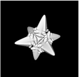
Figures 1 to 3 show snapshots of a typical dendritic structure that has been simulated using the solution techniques described in this paper. These results have been com-puted using an anisotropy parameter ˜ǫ = 0.05, λ = 3.2 and an initial undercooling,
∆, of 0.65 (that isuis set initially everywhere to -0.65). For this run, up to six levels of refinement of the initial8×8×8block (level 0) have been permitted, which pro-vides equivalent resolution to that of a uniform mesh of dimension512×512×512, containing∼ 134.2M cells. An initial spherical seed of solid phase is defined at the centre of the domain ([−200,200]3
) and the evolution of the solution is computed. In this example a fixed time step is used and the spatial adaptivity is based upon the gra-dient of the phase variable. Results were computed on a dual (quad-core) processor workstation with 16Gb of RAM.
Figure 1: snapshot of a typical anisotropic solution, showing theφ = 0.0isosurface at the end of a simulation
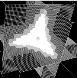
the adapted mesh only, illustrates that mesh coarsening has begun to occur at the centre of the domain: which was originally refined to the maximum level.
5.2
Quantitative comparison with an explicit code
In this section we compare the performance of the implicit, multigrid solver described above with a much simpler explicit model employing forward Euler time-stepping. This solver, full details of which are given elsewhere [22], is also based around the PARAMESH package. Both solvers use the block-based adaptive capabilities of PARAMESH and comparative tests have been conducted on the same multi-processor workstation with up to 4 cores and 8Gb of RAM available. In each case exactly the same equation set is solved however, when using explicit methods, [9, 21], a major constraint in the computation is the time-step restriction in order to assure stability of the scheme. The unconditional stability of the implicit scheme allows much greater time steps to be taken but, even with the efficiency of multigrid, the cost per step is far greater. The purpose of these tests is to ascertain the extent to which this higher computational overhead per time step is compensated by the ability to take larger time steps. However, the comparison also provides a useful check of the solver integrity, provided both explicit and implicit models converge to the same result.
Comparative tests have been run for an initial seed growing into a uniformly under-cooled melt with ∆= 0.65 on a[−200,200]3
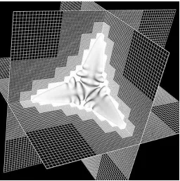
Figure 2: snapshot of the same solution as in Fig. 1, showing the adapted grid as well as theφ= 0.0isosurface
(ǫ˜= 0), in which case a simple spherical morphology results, and anisotropic growth (ǫ˜= 0.05), giving rise to dendrites such as that shown in Figure 1.
In order to show the effect of moving to progressively finer mesh spacing, tests have been conducted for 5-7 levels of refinement, corresponding to minimum mesh sizes ofh= 1.56toh= 0.39respectively on the[−200,200]3
domain employed here. For the explicit model, the maximum stable time-step, as determined by numerical exper-imentation, was 0.15, 0.0375 and 0.009375 for 5, 6 and 7 levels of refinement respec-tively, irrespective of whether the solution was isotropic or anisotropic. Conversely, for the implicit model the selected time step was held constant for all simulations, at 0.15, except the anisotropic case with 7 levels of refinement. In this case the nonlinear multigrid did not always converge and so the step was reduced to 0.06.
On the coarsest meshes employed some differences in the solutions obtained us-ing explicit and implicit methods are observed (of the order 5 % in the position of the dendrite tip), which is most likely due to the structured hexahedral mesh imparting ad-ditional anisotropy into the solution. This problem is well documented in phase-field simulation and has been shown to be most severe when coarse meshes are used, [16]. Convergence to the same result for the explicit and implicit solvers is observed as the mesh spacing is reduced, with the results on level 7 being virtually indistinguishable.
Results of the comparative run time are reported based on the real time required on four cores for the model to reach a (non-dimensional) simulation time oft = 150
and are given in Table 1. Note that, on the coarsest mesh (level 5) the same time step,
Figure 3: snapshot of the locally adapted grid corresponding to the solution shown in Fig. 1
due to the lower computational load per time step, the explicit model clearly performs much better in this case. However, as we move to progressively finer meshes the time step for the explicit model scales, as expected, as h2
, while the time-step for the implicit model remainshindependent. Consequently, with 6 levels of refinement we see similar computational times, while with 7 levels of refinement the implicit scheme clearly performs much better.
Isotropic Anisotropic
h level Explicit Implicit Ratio Explicit Implicit Ratio
1.56 5 2052 6480 3.14 2412 13788 5.78
0.78 6 27108 35064 1.29 42912 47484 1.11 0.39 7 307476 176688 0.57 437832 537912 1.23
Table 1: Comparative execution times required for the explicit and implicit solvers to advance the phase-field simulation tot = 150. Times based on parallel execution on 4 cores.
[image:13.612.124.472.468.546.2][22, 24], that for the much stiffer system that result when chemical, as well as thermal, diffusion is introduced into the crystallization problem, solution via explicit methods becomes infeasible once the ratio of thermal to chemical diffusivity (the Lewis num-ber) becomes significant. Conversely, stiff implicit multigrid methods permit solution in 2-dimensions even when Lewis numbers of order 10000 are used, [25]. Conse-quently, we believe that implicit, multigrid methods are the only way in which such systems can be tackled in 3-dimensions.
5.3
Parallel performance
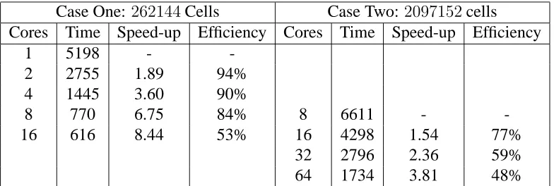
The primary purpose of implementing the three-dimensional solver in parallel using PARAMESH is to allow larger problems to be solved than would otherwise be pos-sible (on a single processor). Before considering the degree to which this has been achieved however it is also informative to assess the efficiency of the underlying par-allel implementation for problems of a fixed size. Table 2 shows the results of two such tests using uniform mesh refinement up to levels 3 and 4 respectively. For the smaller of these two problems it is possible to obtain a parallel efficiency of just over
50% on 16 cores, and for the larger problem an efficiency of just under 50% (rela-tive to the 8 core case) is achieved using 64 cores. As the problem size is increased (by increasing the number of levels of refinement) the memory requirement grows, and so the minimum number of cores needed to run the problem also goes up. The system used for all of the parallel runs in this sub-section consists of dual core AMD processors with up to 2Gb of RAM per core.
Case One: 262144Cells Case Two:2097152cells Cores Time Speed-up Efficiency Cores Time Speed-up Efficiency
1 5198 -
-2 2755 1.89 94%
4 1445 3.60 90%
8 770 6.75 84% 8 6611 -
-16 616 8.44 53% 16 4298 1.54 77%
32 2796 2.36 59%
[image:14.612.103.495.400.532.2]64 1734 3.81 48%
Table 2: Parallel scalability results for the phase-field solver on two problems of fixed sizes
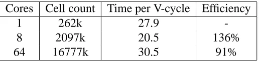
the number of cores is increased by this factor. The execution time of each V-cycle of the multigrid solver grows linearly with the problem size and so, even though the total number of V-cycles is dependent on the mesh size (primarily due to smaller time steps being required on a finer mesh), the execution time per V-cycle should remain constant in each run if the parallel efficiency is100%. Table 3 clearly shows that this parallel efficiency, when the work per core is kept constant, is indeed very good. The figure of 136% for the 8 core case is quite difficult to explain but may be due to the single core runs being adversely affected by other users on the system.
Cores Cell count Time per V-cycle Efficiency
1 262k 27.9
-8 2097k 20.5 136%
[image:15.612.170.428.182.244.2]64 16777k 30.5 91%
Table 3: Parallel scalability results for the phase-field solver as the problem size is scaled with the number of cores
Of course, the primary goal of this work is not to achieve parallel scalability on uniformly refined meshes but to allow a parallel capability for the implicit solution of phase-field problems on locally adapting meshes. Table 4 shows how well this has been achieved by comparing the simulation capability that is possible using a parallel solver with uniform mesh refinement versus the capability that adaptive mesh refine-ment allows. It is clear that, for this particular run (which depends upon the dendrite morphology and the domain size in the adaptive case), the same spatial resolution may be obtained on just 2 cores with adaptivity as on 64 cores without. Similarly, adaptivity permits refinement level 7 to be reached using just 20 cores however the memory requirement for uniform refinement to level 7 (saving the mesh hierarchy for the multigrid solver) would require approximately 4096 cores. Although limits on the cpu time available to us have prevented a full simulation from being completed (and so the results are not shown in Table 4) we have also been able to show that adaptive simulations up to refinement level 8 (equivalent to over 8 billion cells on a uniform grid) are possible using 128 cores.
Cores Uniform Grid Level (Cells) Adaptive Grid Level (Equiv. Cells)
1 3 (262k) 4 (2.1M)
2 5 (16.8M)
8 4 (2.1M) 6 (134.2M)
20 7 (1073.7M)
64 5 (16.8M)
6
Discussion
This paper presents what the authors believe to be the first example of the successful application of parallelism, adaptivity, implicit time-stepping and multigrid together, for the solution of three-dimensional phase-field systems. The work is a natural ex-tension of our earlier results in two space dimensions, [22, 23], where the advantages of implicit time-stepping are shown, provided that the mesh is sufficiently fine and a fast (i.e. multigrid) algebraic solver is implemented. The implementation of the multigrid solver in three dimensions presents no additional mathematical difficulties however the technical problems associated with moving from two to three dimensions are significant. These have been overcome through the use, and further development, of the PARAMESH software library [19, 20].
Results presented show that the development of complex structures, such as den-drites, can be successfully simulated in three dimensions, and that the adaptive data structure permits an efficient representation of the solution fields. Comparison with an existing explicit solver, [22], demonstrates both the accuracy and the potential effi-ciency of the implicit approach. Finally, the parallel performance is shown to be ade-quate to allow a significantly improved capability over the use of either parallelism or adaptivity alone.
Acknowledgement
This work is supported by the Engineering and Physical Sciences Research Council, via grant EP/F010354/1.
References
[1] Barbieri, A & Langer, J S, Predictions of Dendritic Growth Rates in the Lin-earized Solvability Theory. Phys. Rev. A, 39, 5314–5325, 1989.
[2] Bastian, P, Lang, S & Eckstein, K, Parallel Adaptive Multigrid Methods in Plane Linear Elasticity Problems. Numer. Linear Alebr., 4, 153–176, 1997.
[3] Battersby, S E, Cochrane, R F & Mullis, A M, Microstructural evolution and growth velocity-undercooling relationships in the systems Cu, Cu-O and Cu-Sn at high undercooling. J. Mater. Sci., 35, 1365–1373, 2000.
[4] Brandt, A, Multi-Level Adaptive Solutions to Boundary-Value Problems. Math-ematics of Computations, 31(138), 333-390, 1977.
[5] Brener, E, Needle-Crystal Solution in 3-Dimensional Dendritic Growth. Phys. Rev. Lett., 71, 3653–3656, 1993.
[6] George, W L & Warren, J A, A Parallel 3D Dendritic Growth Simulator Using the Phase-Field Method. J. Comput. Phys., 177, 264–283, 2002.
[7] Griebel M & Zumbusch, G, Parallel Multigrid in an Adaptive PDE Solver Based on Hashing and Space-Filling Curves. Parallel Comput., 25, 827–843, 1999. [8] Hu, X L, Li, R & Tang, T, A Multi-Mesh Adaptive Finite Element
Approxima-tion to Phase Field Models. Comm. Comput. Phys., 5, 1012–1029, 2009.
[9] Jeong, J-H, Goldenfeld, N & Dantzig, J A, Phase Field Model for Three-Dimensional Dendritic Growth with Fluid Flow. Phys. Rev. E, 64, 041602, 2001. [10] Jones, A C & Jimack, P K, An Adaptive Multigrid Tool for Elliptic and Parabolic
Systems. Int. J. Numer. Meth. Fluids, 47, 1123–1128, 2005.
[11] Karma, A & Rappel, E-J, Phase-Field Method for Computationally Efficient Modeling of Solidification with Arbitrary Interface Kinetics. Phys. Rev. E, 53, 3017–3020, 1996.
[12] Karma, A & Rappel, E-J, Phase-Field Simulation of Three-Dimensional Den-drites: Is Microscopic Solvability Theory Correct? J. Crystal Growth, 174, 54– 64, 1997.
[13] Karma, A & Rappel, E-J, Quanitative Phase-Field Modeling of Dendritic Growth in Two and Three Dimensions. Phys. Rev. E, 57, 4323–4349, 1998.
[14] McFadden, G B, Wheeler, A A, Braun, R J, Coriell, S R & Sekerka, R F, Phase-Field Models for Anisotropic Interfaces. Phys. Rev. E, 48, 2016–2024, 1993. [15] Mullis, A M, The effect of the ratio of solid to liquid conductivity on the stability
parameter of dendrites within a phase-field model of solidification. Phys. Rev. E, 68, art. no. 011602, 2003
[17] Mullis, A M & Cochrane, R F, A phase field model for spontaneous grain refine-ment in deeply undercooled metallic melts. Acta Mater., 49, 2205–2214, 2001. [18] Mullis, A M, Cochrane, R F, Walker, D J & Battersby, S E, Deformation of
dendrites by fluid flow during rapid solidification. Mater. Sci. Eng. A, 304-306, 245–249, 2001
[19] Olson, K, PARAMESH: A Parallel Adaptive Grid Tool. In Parallel Computa-tional Fluid Dynamics 2005: Theory and Applications, ed. A. Deane et al. (El-sevier), 2006.
[20] Olson, K, PARAMESH tutorial. www.physics.drexel.edu/˜olson/paramesh-doc/Users manual/amr tutorial.html, accessed 10 December 2008.
[21] Provatas, N, Goldenfeld, N & Dantzig, J A, Adaptive Mesh refinement Computa-tion of SolidificaComputa-tion Microstructures Using Dynamic data Structures. J. Comput. Phys., 148, 265–290, 1999.
[22] Rosam, J, A Fully Implicit, Fully Adaptive Multigrid Method for Multiscale Phase-Field Modelling. PhD Thesis, University of Leeds, 2007.
[23] Rosam, J, Jimack, P K & Mullis, M M, A Fully Implicit, Fully Adaptive Time and Space Discretisation Method for Phase-Field Simulation of Binary Alloy Solidification. J. Comp. Phys., 225, 1271–1287, 2007
[24] Rosam, J, Jimack, P K & Mullis, A M, An Adaptive, Fully Implicit, Multigrid Phase-Field Model for the Quantitative Simulation of Non-isothermal Binary Alloy Solidification. Acta Mat., 56, 4559–4569, 2008.
[25] Rosam, J, Jimack, P K & Mullis, A M, Quantitative phase-field modelling of thermo-solutal solidification at high Lewis number. Phys. Rev. E, 79, art. no. 030601, 2009
[26] Suwa, Y, Saito, Y & Onodera, H, Parallel computer simulation of three-dimensional grain growth using the multi-phase-field model . Mater. Trans., 49, 704–709, 2008.
[27] Touheed, N, Selwood, P, Jimack, P K & Berzins, M, A Comparison of Some Dy-namic Load-Balancing Algorithms for a Parallel Adaptive Flow Solver. Parallel Computing, 26, 1535–1554, 2000.
[28] Trottenberg, U, Oosterlee, C, Sch¨uller, A, Multigrid. Academic Press 2001 [29] Warren, J A & Boettinger W J, Prediction of Dentritic Growth and
Microseg-regation Patterns in a Binary Alloy using the Phase-Field Method. Acta Matall. Mater., 43, 689–703, 1995.
[30] Wheeler, A A, Murray, B T & Schaefer, R J, Computation of Dendrites Using a Phase-Field Model. Physica D, 66, 243–262, 1993.