Balancing Authority Area Model and its Application to the Design of Adaptive AGC Systems

City, University of London Institutional Repository

Citation

: Apostolopoulou, D., Sauer, P. W. & Dominguez-Garcia, A. D. (2016). Balancing

Authority Area Model and its Application to the Design of Adaptive AGC Systems. IEEE

Transactions on Power Systems, 31(5), pp. 3756-3764. doi: 10.1109/TPWRS.2015.2506181

This is the accepted version of the paper.

This version of the publication may differ from the final published

version.

Permanent repository link:

http://openaccess.city.ac.uk/19252/

Link to published version

: http://dx.doi.org/10.1109/TPWRS.2015.2506181

Copyright and reuse:

City Research Online aims to make research

outputs of City, University of London available to a wider audience.

Copyright and Moral Rights remain with the author(s) and/or copyright

holders. URLs from City Research Online may be freely distributed and

linked to.

Balancing Authority Area Model and its Application

to the Design of Adaptive AGC Systems

Dimitra Apostolopoulou,

Student Member

,

IEEE

, Peter W. Sauer,

Fellow Member

,

IEEE

, and

Alejandro D. Dom´ınguez-Garc´ıa

Member

,

IEEE

Abstract—In this paper, we develop a reduced-order model for synchronous generator dynamics via selective modal analysis. Then, we use this reduced-order model to formulate a balancing authority (BA) area dynamic model. Next, we use the BA area model to design an adaptive automatic generation control (AGC) scheme, with self-tuning gain, that decreases the amount of regulation needed and potentially reduces the associated costs. In particular, we use the BA area model to derive a relationship between the actual frequency response characteristic (AFRC) of the BA area, the area control error, the system frequency, and the total generation. We make use of this relationship to estimate the AFRC online, and set the frequency bias factor equal to the online estimation. As a result, the AGC system is driven by the exact number of MW needed to restore the system frequency and the real power interchange to the desired values. We demonstrate the proposed ideas with a single machine infinite bus, the 9-bus 3-machine Western Electricity Coordinating Council (WECC), and a 140-bus 48-machine systems.

Index Terms—Reduced-Order Synchronous Generator Model, Balancing Authority Area Model, Adaptive Automatic Genera-tion Control, Actual Frequency Response Characteristic.

I. INTRODUCTION

The appropriate granularity necessary to describe power sys-tem components, e.g., synchronous generators, is determined by the type of phenomena that need to be studied. For example, simplified models, such as the classical model for describing generators dynamics, may be used in studies where the focus is on slow-varying transients. The general idea behind simplified models is to approximate the behavior of selected dynamics, by means of various integral manifolds, without having to explicitly solve the full set of differential equations. In the same vein, reduced-order modeling techniques may be used at the balancing authority (BA) area level to describe the BA area dynamic behavior.

Since the slower-varying transients are sufficient for describ-ing the BA area dynamic behavior, such simplified models may be used in the design of new automatic generation control (AGC) systems. The role of AGC is to maintain the system

The authors are with the Department of Electrical and Computer Engineer-ing of the University of Illinois at Urbana-Champaign, Urbana, IL 61801, USA. E-mail:{apostol2, aledan, psauer}@illinois.edu.

The work of Apostolopoulou and Sauer was supported in part the US Departments of Energy and Homeland Security through the Trustworthy Cyber Infrastructure for the Power Grid, the US Department of Energy GEARED Initiative, the Power Systems Engineering Research Center (PSERC), and the Grainger Foundation Endowments to the University of Illinois. The work of Dom´ınguez-Garc´ıa was supported in part by the National Science Foundation (NSF) under CAREER Award CAR-0954420 and NSF award ECCS-CPS-1135598.

frequency at the nominal value and the power net interchange between BA areas at the scheduled values. There is a need for new AGC system designs, since studies show that demand for AGC will increase due to larger net load variations caused by the deepening penetration of renewable-based resources [1]. Thus, to cope with the aforementioned challenges, either increased requirements of AGC system reserves, which are expensive, are necessary, or new designs in the AGC system that enhance its efficiency are mandated. Most BA areas implement tie-line bias control, and the AGC command is driven by the value of the area control error (ACE), which includes the deviation of the sum of tie line flows between the BA areas from the scheduled values and their obligation to support frequency.

In order to prevent the AGC system from “fighting” the area’s natural response, the BA area obligation to support frequency is included in the ACE calculation. This term includes the frequency bias factor, which in the ideal case reflects the actual frequency response characteristic (AFRC) of the BA area. The AFRC is the change in frequency that occurs for a change in load-generation balance in an interconnection. Independent system operators usually use the 1% of peak load method to determine the frequency bias factor, which leads to frequency bias factors greater than the AFRC and causes over-regulation. A method that estimates the AFRC and uses this value as the frequency bias factor increases the efficiency of the AGC system. We may estimate the AFRC of a BA area by using a power system model, simplified or not, to derive a relationship between the AFRC and system variables.

We use the proposed reduced-order model to derive a set of differential equations that describe a BA area dynamics; an objective is that this set of equations depends only on BA area variables. To this end, we use optimization techniques and define the BA area droop and damping coefficients. The derived model approximates better the BA area behavior than other BA area dynamic models, where the droop and damping coefficients are the summation of each generator droop and damping values [4]. We compare the BA area model with others, such as the 9-state model, and verify that it provides a good approximation of the actual system state.

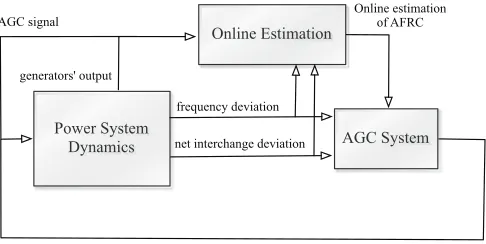
Next, we use the BA area model, described above, to design an adaptive AGC system. Such a model is sufficient to model the system dynamics for AGC implementation purposes, since the output command of the latter is the total generation needed in the BA area to restore the system frequency and the net interchange between BA areas to the desired values. In this regard, models that do not consider each generator states, but only the BA area variables are sufficient. We modify the AGC system design and include an adaptive proportional controller with self-tuning gain that reflects the system AFRC. To imple-ment such a controller, we estimate the AFRC online by using the proposed BA area model, and then we derive a relationship between the AFRC, the system frequency, the ACE and the total generation. We select the sliding exponentially weighted window blockwise least-squares (SEWBLS) algorithm for the online estimation of the AFRC (see, e.g., [5]). Such an algorithm keeps the computational complexity to a fixed level by keeping the length of the sliding window fixed. In order to exploit the advantages of forgetting estimation techniques and improve the tracking capability of the algorithm the SEW-BLS introduces an exponential weighting technique. This is especially useful for the case in which the system experiences a change in the operating point during the time window in which measurements are obtained. The performance of the SEWBLS algorithm depends on the length of the sliding window. For systems with parameter changes, such as power systems, the window length should be adjusted accordingly so that out-of-date information from past measurements can be discarded effectively and achieve fast tracking of the changed parameters based on the latest measurements. In this paper, we show that the proposed estimation technique provides a good approximation of the AFRC and that when used in the ACE calculation the system frequency converges faster to the nominal value. A block diagram of the proposed adaptive AGC system is depicted in Fig. 1.

Several papers are dedicated to the development of reduced-order models for system components. For example, in [6], a method is proposed for reducing the state matrices of a linear system by keeping the dominant eigenvalues and eigenvectors of the original system. A similar approach is given in [3], where the authors use selective modal analysis to construct a simplified model. A number of papers have focused on the use of simplified models and the design of AGC systems. A description of the AGC system role and limitations is given in [7], where the authors also mention why the AFRC is a good approximation to the frequency bias factor (in the context of ACE calculation). A discussion of

Power System

Dynamics AGC System Online Estimation

generators' output

frequency deviation

net interchange deviation AGC signal

[image:3.612.320.563.63.185.2]

Online estimation of AFRC

Fig. 1: Block diagram of the adaptive AGC system.

the current practices for calculating frequency bias factors, their limitations, and the proposal of a new method for sizing these factors is given in [8]. In [9], the authors discuss issues related to variable generation management, and adaptive AGC unit tuning, to make the AGC system more efficient. The authors in [10] propose an optimization technique to determine parameters in the AGC system, such as gain controllers, to increase its efficiency. In [11], the authors propose a stochastic optimal relaxed AGC system, which takes into account North american Electric Reliability Corporation (NERC) frequency performance standards, and reduces control cost by tuning the relaxation factors online.

The contributions of this paper may be outlined as follows: the development of (i) a synchronous generator reduced-order model, (ii) a BA area model, and (iii) an adaptive AGC system. The advantages of (i) compared to other works (e.g., [3], [6]) are that it is simpler than the 9-state model, approximates the system behavior in satisfactory levels, provides better accuracy compared to the classical model, and has lower computational burden compared to other reduced-order models, since only the eigenvalues of a submatrix are needed. Next, we use (i) to develop (ii). A systematic way to develop a BA area model that represents the BA area dynamic behavior is missing from the literature. The value of the BA area model is that it is derived directly from the individual generator models and not in a heuristic way. The typical BA area model (e.g., [2], [4], [12]) uses the heuristic approach of adding the individual damping and droop coefficients of the individual generators to determine the damping and droop of the BA area respectively. The developed BA area model may be used in various applications where the dynamic behavior of a BA area needs to be represented. In this paper, we use it to derive (iii), where the AFRC is estimated. The calculation of the AFRC is a step forward in conducting the frequency response assess-ment in a more scientific way and not with heuristic formulas (e.g., [13]). In addition, the proposed adaptive AGC system may be actually implemented in real large-scale systems, as validated in the numerical results section, in contrast with other advanced AGC system designs, e.g., [10], [11], where the computational burden is large. Since, the AGC system is implemented in fast timescales, 2-4 seconds, such designs are hard to be implemented in real systems.

model. In Section III, we derive the proposed models for the synchronous generator and BA area dynamic behavior. In Section IV, we present the proposed adaptive AGC system. To this end, we obtain a relationship between the ACE, the frequency deviation, the total generation and the AFRC at each time instant, and use it to estimate the system AFRC online via a SEWBLS algorithm. In Section V, we demonstrate the proposed ideas on a single machine infinite bus system, the 9-bus 3-machine Western Electricity Coordinating Council (WECC) system, and a 140-bus 48-machine system. Finally, we provide some concluding remarks and discuss the direction for future research in Section VI.

II. PRELIMINARIES

In this section, we provide models for the synchronous generator and AGC dynamics, and the network. These models are the starting point for the developments in subsequent sections.

A. Synchronous Generator Dynamics

The analysis starts with a synchronous generator dynamic model without the fast stator/network dynamics — often called the “two-axis” model. For the ith _{synchronous generator, the}

nine states are: the field flux linkageE′_qi, the damper winding flux linkage E_d′_i, the rotor electrical angular position δi, the rotor electrical angular velocity ωi, the scaled field voltage

Ef di, the stabilizer feedback variable Rfi, the scaled output

of the amplifierVRi, the scaled mechanical torque to the shaft TMi, and the mechanical powerPSVi (see, e.g., [14, p.140]).

The evolution of these variables is determined by:

T_do′ _idE

′

qi

dt = −E

′

qi−(Xdi−X ′

di)Idi+Ef di, (1)

T_qo′ _idE

′

di

dt = −E

′

di+ (Xqi−X ′

qi)Iqi, (2) dδi

dt = ωi−ωs, (3)

2Hi ωs

dωi

dt = TMi−E ′

diIdi−E ′

qiIqi

−(Xqi−X ′

di)IqiIdi−Di(ωi−ωs),(4) TEi

dEf di

dt = −(KEi+ 0.0039e

1.555E_{f di)} Ef di

+VRi, (5)

TFi dRfi

dt = −Rfi+ KFi

TFi

Ef di, (6)

TAi dVRi

dt = −VRi+KAiRfi−

KAiKFi TFi

Ef di

+KAi(Vrefi−Vi), (7) TCHi

dTMi

dt = −TMi+PSVi, (8)

TSVi dPSVi

dt = −PSVi+PCi−

1

RDi

ωi

ωs

−1, (9) where the synchronous reference rotating speed isωsand the

inertia constant is Hi; the governor time constant isTSVi; the

d-axis (q-axis) component of the stator current is Idi (Iqi);

the voltage magnitude at bus i is Vi; and the parameter PCi

is an input provided by the AGC and is given in (13). The definitions of the machine parameters may be found in [14].

In addition to (1)-(9), we also have a set of algebraic equations

Viejθi_{+ (RS} i+jX

′

di)(Idi+jIqi)e j(δi−π2)

−

Ed′i+ (X ′

qi−X ′

di)Iqi+jE ′

qi

ej(δi−π2)= 0, (10)

whereθi is the voltage phase angle at busi.

B. AGC System

Let A _{={1,2, . . . , M} denote the set of BA areas in an}

interconnected power system, and for each m∈ A_{, let} A_m

denote the set of BA areas directly connected to BA aream; then, the ACE for aream,ACEm, is given by

ACEm= X

m′_∈A m

∆Pmm′−bm∆fm, (11)

where ∆Pmm′ is the difference between the actual and the

scheduled power transfer from BA area m to BA area m′,

bm is the frequency bias factor, and ∆fm is the frequency deviation from the nominal value.

LetG_{m denote the set of all generators in BA aream, and}

define a new state for the system, zm, which is the sum of the AGC commands sent to generators in BA area m, i.e.,

P

i∈GmPCi; then its evolution is given by dzm

dt =−ACEm. (12)

Each generatoriin BA area m participates in the AGC by a participation factorκm_i , which is determined in various ways (see, e.g., [15], [16]). Thus, the AGC command PCi, used

in (9), is determined by

PCi=P ⋆ Gi+κ

m i (zm−

X

j∈G_m

P_G⋆_j), (13)

where P⋆

Gi is the economic dispatch signal for generator i,

andP

i∈Gmκ m i = 1.

C. Network

Let PLi represent the real power load at bus i. Further,

let QGi and QLi denote the reactive power supplied by the

synchronous generator and demanded by the load at bus i, respectively. Then, we model the network using the standard nonlinear power flow formulation (see, e.g., [14]); thus, for theith _{bus, we have that}

(PGi−PLi) +j(QGi−QLi) =

Pn

k=1ViVk(Gik−jBik)ej(θi−θk), (14) whereGik+jBik is the(i, k)entry of the network admittance matrix.

III. SIMPLIFIEDPOWERSYSTEMDYNAMICMODELS

A. Synchronous Generator Reduced-Order Model

We use the 9-state model in (1)-(10) to obtain a reduced-order three-state model with δi, ωi, and PSVi. We wish to

keep (3), (4), and (9), and substitute the remaining differential equations with algebraic ones. To do so, we use concepts from SMA, which is a technique used to simplify high-order linear systems (see, e.g., [3]). Let xi = [rTi , ζiT]T, where ri =

[δi, ωi, PSVi]

T_{, and ζi = [E}′

qi, E ′

di, Ef di, Rfi, VRi, TMi] T_;

yi = [Vi, θi]T; y˜i = [Idi, Iqi]

T_{; and u}

i = PCi. We may

linearize the system described in (1)-(10) along a nominal trajectory(x⋆

i, yi⋆,y˜⋆i, u⋆i). Sufficiently small variations around

the system nominal trajectory may be approximated by

∆ ˙xi = A1i∆xi+A2i∆yi+A3i∆˜yi+Bi∆ui, (15)

0 = C1i∆xi+C2i∆yi+C3i∆˜yi, (16)

where the matrices A1i, A2i, A3i, Bi, C1i, C2i, andC3i are

defined appropriately and evaluated along the nominal trajec-tory as the partial derivatives of the functions given in (1)-(10). We assume the nominal trajectory is well behaved in the sense thatC3i is invertible; thus, we may solve for∆˜yi. We

substi-tute∆˜yi in (15) and obtain∆ ˙xi=Ai∆xi+Di∆yi+Bi∆ui, whereAi=A1i−A3iC

−1

3i C1i andDi =A2i−A3iC −1 3i C2i.

We now partition the statesxiinto relevantriand less relevant

states ζi, and rewrite the system into partitioned form as

follows:

∆ ˙ri

∆ ˙ζi

=

A11i A12i A21i A22i

∆ri

∆ζi

+

D1i D2i

∆yi+

B1i B2i

∆ui. (17)

The idea behind SMA is to approximate the behavior of the relevant states, ∆ri, with a set of differential equations that

contain only ∆ri and ∆yi, i.e., to substitute the differential

equations of ∆ζi with a set of algebraic equations. We do

so by “freezing” the less relevant states, with the help of eigenanalysis methods. More specifically, we select the three natural modes which define the dynamic pattern of interest. These are: (i) the two complex eigenvalues, where the relative participation of ∆δi and∆ωi is high; and (ii) the real eigen-value, where the contribution of ∆PSVi is high. One way to

calculate the three eigenvalues is by using the entire matrixAi; however, such an approach increases the computational burden in large-scale systems. Instead, we choose the submatirxA11i

to determine the values of the three modes. It has been shown in [17] that this matrix yields good approximations to the frequencies of the swing modes.

By solving (17) for∆ζi, we obtain that

∆ζi = (sI−A22i) −1_A

21i∆ri+ (sI−A22i) −1_D

2i∆yi

+(sI−A22i) −1_B

2i∆ui,

whereI is the identity matrix, ands is the Laplace operator. However, as it may be seen from (1)-(10), the value of B2i is

zero. Thus, we have that

∆ζi = (sI−A22i) −1

A21i∆ri+ (sI−A22i) −1

D2i∆yi.

We fix sto the values corresponding to the three eigenvalues and obtain a set of linear equations∆ζi=Aζi∆ri+Dζi∆yi.

In particular, Aζi satisfies the property Aζivj = Zi(λj)vj,

for j = 1, . . . ,3, where Zi(s) = (sI −A22i) −1_A

21i, λj

is the eigenvalue corresponding to mode j, and vj is the right eigenvector of mode j. In the case of a conjugate pair of complex eigenvalues the equation is slightly different; the details may be found in [3]. For simplicity, we setDζi=D2i.

We wish to include the mechanical powerPSViin the swing

equation, as given in (4), instead of the scaled mechanical torque to the shaftTMi. To this end, we write (8) as(sTCHi+

1)TMi =PSVi. If we set s = 0, then TMi = PSVi. This is

equivalent to a singular perturbation of the fast variableTMi.

To sum up, we use the small3×3matrixA11i to calculate

the desired eigenvalues and determine Aζi and Dζi. The

overall reduced-order model for generatori is now given by

dδi

dt = ωi−ωs, (18)

2Hi ωs

dωi

dt = PSVi−PGi−Di(ωi−ωs), (19) TSVi

dPSVi

dt = −PSVi+PCi−

1

RDi

ωi

ωs−1

, (20)

ζi = ζi⋆+Aζi∆ri+Dζi∆yi, (21)

where ζ⋆

i is the value of ζi at the nominal trajectory

(x⋆

i, yi⋆,y˜⋆i, u⋆i), with the algebraic equations given in (10) and

(14). We denote byPGi =E ′

diIdi+E ′

qiIqi+(Xqi−X ′

di)IqiIdi,

the real power generation at busi.

We compare the proposed reduced-order model in (18)-(21) with the classical model (e.g., [14]). The classical model may be derived by settings= 0for the fast dynamics ands→ ∞

for the slow dynamics. Thus, the approximation of the 9-state model is better in the case of the proposed reduced model, where values that describe the dynamic pattern of interest are used in the Laplace operator.

B. BA Area Model

For each generator i, we use the proposed reduced-order model in (18)-(21). Define ∆ωi =ωi−ωs,Mi = 2Hi

ωs , and

˜

RDi =RDiωs, then we have that

dδi

dt = ∆ωi, (22)

Mid∆ωi

dt = PSVi−PGi−Di∆ωi, (23) TSVi

dPSVi

dt = −PSVi+PCi−

1 ˜

RDi

∆ωi, (24)

with the algebraic equations in (10), (14), and (21). For each BA aream∈A_{, we define}

δm₌

P

i∈G_mMiδi

P

i∈G_mMi

, ∆ωm₌

P

i∈G_mMi∆ωi

P

i∈G_mMi

,

P_SVm = X

i∈G_m

PSVi, P m G =

X

i∈G_m

PGi,

zm= X

i∈G_m

PCi, M

m₌ X

i∈G_m

We add (22)-(24) for all generators inG_{m to obtain} dδm

dt = ∆ω

m_{, (25)}

Mmd∆ω m

dt = P

m

SV −PGm−

X

i∈G_m

Di∆ωi, (26)

X

i∈G_m

TSVi dPSVi

dt = −P

m

SV +zm−

X

i∈G_m

1 ˜

RDi

∆ωi. (27)

We modify (26)-(27) by using the definitions for the BA area variable∆ωm, and obtain

Mmd∆ω m

dt = P

m

SV −PGm−

X

i∈G_m

Di Mi

Mm∆ωm

+ X

i∈G_m

_X

j∈G_m

i6=j Dj Mj

Mi∆ωi, (28)

X

i∈Gm TSVi

dPSVi

dt = −P

m

SV +zm−

X

i∈Gm

1 ˜

RDiMi

Mm_∆ωm

+ X

i∈G_m

_X

j∈G_m

i6=j

1 ˜

RDjMj

Mi∆ωi. (29)

We wish to substitute the terms referring to each syn-chronous generating unit with a BA area variable. To do so from (28)-(29), we wish that P

j1∈Gm i6=j1

Dj1

Mj1 =

P

j2∈Gm i6=j2

Dj2

Mj2,

P

j1∈Gm i6=j1

1 ˜ R_Dj

1Mj1 =P

j2∈Gm i6=j2

1 ˜ R_Dj

2Mj2

, andTSVj1 = TSVj2

for alli, j1, j2∈Gm. We may rewrite the equations as Di

Mi = c1,constant,∀i∈Gm, (30)

1 ˜

RDiMi

= c2,constant,∀i∈Gm, (31) TSVi = c3,constant,∀i∈Gm; (32)

from where it follows that

Mmd∆ω m

dt = P

m

SV −PGm−c1Mm∆ωm, (33) c3

dPSVm

dt = −P

m

SV +zm−c2Mm∆ωm. (34) In order to determine the parametersc1,c2andc3, we wish to minimize the euclidean norm of the errors of the ratios given in (30)-(32); however, there is a constraint relating c1 and c2. The deviations of the rotor angular speeds from the nominal value are the same for each generatori∈G_{mand the}

BA area. We use the reduced-order model for each generatori, given in (22)-(24), and the Laplace transformation, to obtain

s2TSVi+s(Mi∆ωi+PGiTSVi+DiTSVi∆ωi)−PCi

+ 1 ˜

RDi

∆ωi+PGi+Di∆ωi= 0.

Whent→ ∞, thens→0, and we have

1 ˜

RDi

+Di

∆ωi=PCi−PGi =−(PGi(t)−PGi(0)),

since PCi(t) =PGi(0), when the AGC system model is not

considered. We use (33), (34), and in a similar way find the

relationship that holds for t→ ∞for the BA aream. Since, ∆ωi(t) = ∆ωm_(t),∀i∈G

mas t→ ∞, we have PGi(t)−PGi(0)

1 ˜

RDi +Di

= P

m

G(t)−PGm(0)

(c1+c2)Mm

,∀i∈G_{m. (35)}

Since P

i∈G_m(PGi(t)−PGi(0)) =P m

G(t)−PGm(0), then by

adding (35) for all generatorsi∈G_{m, we may derive that}

X

i∈G_m

1 ˜

RDi

+Di

= (c1+c2)Mm.

Now, we may construct the constrained optimization problems to determine the parametersc1,c2, andc3, given in (33)-(34), as follows

minimize

c1,c2

X

i∈G_m

c1− Di Mi

2

+ X

i∈G_m

c2−

1

MiRD˜ i

2

such that X

i∈G_m

1 ˜

RDi

+Di= (c1+c2)Mm;

(36)

and

minimize

c3

X

i∈Gm

c3−TSVi

2

. (37)

By solving the optimization problems in (36) and (37) we obtain

Dm _=c

1Mm=

1 2|G_m|

X

i∈G_m

Mm Mi (Di−

1 ˜ RDi ) +1 2 X

i∈G_m

1 ˜

RDi

+Di,

1 ˜ Rm

D

=c2Mm=

1 2

X

i∈G_m

1 ˜

RDi

+Di

− 1

2|G_m|

X

i∈G_m

Mm Mi

(Di− 1

˜

RDi

),

T_SVm =c3=

P

i∈G_mTSVi

|G_m| ,

where|G_{m| the cardinality of the set}G_m.

We may describe the BA area dynamic behavior by

dδm

dt = ∆ω

m_{, (38)}

Mmd∆ω m

dt = P

m

SV −PGm−Dm∆ωm, (39) T_SVm dPSVm

dt = −P

m

SV +zm−

1 ˜

Rm D

∆ωm, (40)

where Pm

G =

P

i∈Gm

Pn

k=1ViVk Gikcos(θi − θk) + Biksin(θi−θk)

+P_Lm, withP_Lmthe BA areamtotal load.

IV. ADAPTIVEAGC SYSTEM

A. AFRC Determination

We now use (38)-(40), the dynamics of a single BA area, to calculate its AFRC. The AFRC of BA area m is equal to

βm=−2π(_R˜1m D

+Dm_{) =−2π}P

i∈G_m

1 ˜

R_Di +Di

. For the case when the frequency bias factor is set to be equal to the AFRC, we have non-interactive control, which is a fair control in the sense that the BA area in which the load disturbance has occurred is the only one that reacts to restore the frequency and net tie flow to the desired values.

More specifically, we show that under some assumptions the optimal value for the frequency bias factor is the AFRC. We definePm

G =PGm0+ ∆P

m

L + ∆Plossesm , wherePGm0 denotes the total generation of BA area m in steady state. Similarly, we have zm = zm0 + ∆zm. At steady state, the following relationship holds: zm0 = P

m

G0. As in (35), we may obtain a similar relationship for the entire BA area m withs = 0, by using (38)-(40). We denote ∆ωm_{= 2π∆fm, and at time} t=k, we have

βm∆fm(k) + ∆zm(k)−∆PLm−∆Plossesm = 0. (41)

The AGC system algorithm is essentially an integral controller, which is working in discrete form by placing a sample & hold circuit between the AGC and the power system (commands to generators are sent every 2 to 4 seconds). Then, for one BA area, we rewrite the AGC system given in (12) by using (11), and Euler’s method:∆z(k+ 1)−∆z(k) =b∆f(k). So, ∆z(k) =bPk−1

i=0 ∆f(i). We use (41) and the aforementioned AGC algorithm, and for∆f(0) = ∆PL+∆Plosses

β , with∆z(0) =

0, we see that∆f(1) = 0forb=β. In such a case, ACE is corrected in only one control period [18]. Numerical results of this claim may be found in [19].

Since d∆_dtωm = 2πd∆fm

dt , we may combine (39) and (40)

into one equation using the Laplace transformation, and ig-noring the second-order terms since they are negligible due to the system inertia. Thus, we have that

s2π(Mm+DmT_SVm)∆fm−βm∆fm=

zm−(1 +sT_SVm)P_Gm. (42) We use (42) to describe a BA area dynamic behavior, and exploit it to derive a relationship between the AFRC, the ACE, the frequency and the total generation of the BA area.

B. Online Estimation of AFRC

In order to estimate the AFRC, we use (42) in combination with (12), and neglect the newly inserted second-order terms, to obtain

ACEm=sβm∆fm−sP_Gm. (43)

With the introduction of phasor measurement units (PMUs), we can assume that the time elapsed between two consecutive measurements,h, is very small; thus, we may approximate the derivatives in (43) as follows. For every step k, referring to time instantt=kh, we have

βm(k) = ACEm(k) +

Pm

G(k)−PGm(k−1) h ∆fm(k)−∆fm(k−1)

h

. (44)

We use the SEWBLS algorithm for the online estimation of

βm — the AFRC of BA aream(see, e.g., [5]).

In order to formulate our problem, we introduce the follow-ing variables: χ(k) = φ(k)βm(k) and w(k) =χ(k) +v(k), where χ(k) is the system output, w(k) is the measured output andv(k)is a zero-mean white Gaussian sequence that accounts for measurements noise and modeling errors. We have thatφ(k)is the denominator, andχ(k)is the nominator of (44), respectively. The SEWBLS solution is

ˆ

βm(k) =

(φk_k−L+1)TΛkk−L+1φkk−L+1

−1

(φk_k−L+1)T_Λk

k−L+1wkk−L+1

, (45)

whereφk

k−L+1= [φ(k−L+ 1), φ(k−L+ 2), . . . , φ(k)]T, and

Λk

k−L+1 is anL×Ldiagonal matrix with diagonal elements being the forgetting factors, λL−1_{, λ}L−2_{, . . . , λ}0_{. The values} ofλvary from0to1. After several tests, we concluded that a window length ofL= 10min provides good results in terms of convergence speed and accuracy.

V. NUMERICALRESULTS

In this section, we present several numerical studies to demonstrate the proposed ideas and make several comparisons to alternative approaches in the literature. First, we show that the proposed reduced synchronous generator model provides a good approximation to the 9-state model. In addition, we show that the determination of the parametersDm_andR˜m

Dfor

a BA areamprovides a satisfactory description of the system dynamic behavior. We verify that the proposed methodology yields an accurate estimation of the system AFRC, and show the benefits of setting the estimated AFRC as the frequency bias factor in an adaptive AGC system.

A. Single-Machine Infinite-Bus Power System

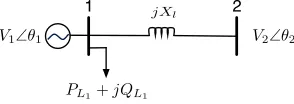
We illustrate the differences between: (i) the proposed reduced-order model in (18)-(21), (ii) the conventional 9-state model in (1)-(10), (iii) the classical model with the governor dynamics, and (iv) the classical model without the governor dynamics. To this end, we simulate the behavior of these models in the context of the single-machine infinite-bus (SMIB) test system, depicted in Fig. 2. The voltage at bus 2 is fixed at1∠0; the machine, network, and load parameter values for this example are as follows: the system MVA base is 100; the synchronous speed isωs= 377rad/s; the machine shaft inertia constant is H = 23.64; the machine damping coefficient is D = 0.0125; the machine impedances are

Xd = 0.146,X_d′ = 0.0608,X_q′ = 0.1969, andXq = 0.8645; the governor droop isRD= 0.05; and the stator, rotor, voltage regulator, exciter, and governor parameters are T_do′ = 8.96,

1 2

V_1∠θ₁ V_2∠θ₂

[image:7.612.364.511.664.716.2]

P_L1+jQ_L1 jXl

9-state model Reduced-order model Classical model with governor Classical model −0.2151_±j2.9256 ₋0.2556_±j3.0082 ₋0.0542_±j3.5146 ₋0.0500_±j3.4849

[image:8.612.74.268.120.208.2]

−0_.5156 ₋0_.5163 ₋0_.4916 ₋

TABLE I: Eigenvalues for the four different models.

t_[s]

0 5 10 15 20 25 30

ω

[r

ad

/s

]

376 377 378 379

proposed reduced-order model 9-state model

classical model with governor classical model

Fig. 3: Rotor electrical angular velocity ω for the three synchronous generator models.

T′

qo= 0.31,TSV = 2,TF = 0.35,KF = 0.063,TE = 0.314, KE = 1, TA = 0.2, and KA = 20. The network impedance between bus 1 and2 is Xl = 0.5. We solve the power flow equations and the machine algebraic equations such that the synchronous generator output in bus 1 isPG1= 0.8, the load in bus 1 is PL1+jQL1 = 1 +j0.5, the voltage magnitude in bus 1 is V1= 0.871.

We choose the SMIB system, since the network impedances are comparable with the machine stator reactances, and thus the proposed reduced-order model yields the worst results with this system. We demonstrate that even in this worst-case scenario, the proposed model provides a very good approximation of the system behavior. We change the load in bus1fromPL1 = 1toPL1= 1.3, and plot the rotor electrical angular velocity of Generator 1 in Fig. 3. We consider the 9-state model as reference and notice that, as we make further simplifications, we lose accuracy in the representation of the actual system behavior. The proposed reduced-order model is very close in terms of damping and frequency of oscil-lations with the 9-state model, in contrast with the classical model with and without the governor dynamics. We may explain this fact by linearizing the four models. The damping and frequency of oscillations of ω are determined by the eigenvalues in which ∆δ, ∆ω, and ∆PSV have the largest participation. The participation of a system state to a mode (eigenvalue) is determined by the participation matrix [3]. In our proposed reduced-order model, the three eigenvalues

2 7 8 9 3

5 6

4

1

G₁ G

[image:8.612.331.529.123.209.2]

2 G3

Fig. 4: One-line diagram of the WECC three-machine nine-bus power system.

t_[s]

0 20 40 60 80 100

ω1

[r

ad

/s

]

376.5 377 377.5 378

proposed reduced-order model 9-state model

PowerWorld model

Fig. 5: Rotor electrical angular speed of Generator 1.

that are associated with ∆δ, ∆ω, and ∆PSV, are close to those of the 9-state model, since that is the way the reduced-order model was constructed. In contrast, the eigenvalues of the classical model with the governor, where ∆δ, ∆ω, and ∆PSV have the largest participation, do not match those of the 9-state model. More specifically, we show the values of the aforementioned eigenvalues in Table I.

B. Three-Machine Nine-Bus Power System

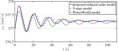
1) Synchronous Generator Reduced-Order Model: We compare the proposed reduced-order synchronous generator model with the PowerWorld dynamic simulation software, which is well-established in the industry, (e.g., [20]) with the standard three-machine-nine-bus WECC power system model, the online diagram of which is depicted in Fig. 4. The system contains three synchronous generating units in buses 1, 2 and 3, and loads in buses 5, 6 and 8; the machine, network and load parameter values may be found in [14]. More specifically, we decrease the load in bus 5 by0.05pu. In the PowerWorld software for the machine model we choose the GENPWTwoAxis model, for the exciter the IEET1 model, for the governor the TGOV1 model, and assign the parameters for the generators as specified in [14]. In this example, we do not include the AGC system; thus the system frequency does not converge to the nominal value. In Fig. 5, we show the rotor electrical angular speed of Generator 1, ω1, calculated with the proposed reduced-order synchronous generator model, the 9-state model, and the PowerWorld model. We may notice that the results of the three models are very close; thus, the proposed reduced-order model provides a good approximation of the synchronous generator dynamic behavior. We also notice that the proposed-reduced order model provides a better approximation of the 9-state model in the WECC power system compared to the SMIB system. The reason is that the network smooths the errors introduced.

2) BA area model: We also use the three-machine-nine-bus WECC power system model to illustrate the proposed BA area model and adaptive AGC system. We consider the system as one BA area and model the system behavior with the proposed model in (38)-(40), which we refer to as method (i). We compare the behavior of the proposed model, with that of a similar model by settingDm =P

i∈G_mDi, _R˜1m D

[image:8.612.90.260.593.713.2]

0 20 40 60 80 100 376.5

377 377.5 378 378.5 379 379.5

ω

[r

a

d

/

s]

t[s]

[image:9.612.68.269.60.146.2]

(i) (ii) (iii)

Fig. 6: Speed of center of inertia with the three methods.

P

i∈G_{m R}˜1

Di, and T m SV =

P

i∈GmTSVi

|G_m| , which is commonly

found in the literature [4]; this is referred to as method (ii). The benchmark model is the 9-state model described in (1)-(10), which we use to calculate the speed of the center of inertia, and refer to it as method (iii). In Fig. 6, we depict the speed of center of inertia calculated with the three methods. In this example, we do not include the AGC system, which is why ω does not converge to the synchronous speed. We notice that the approximation of the BA area dynamics with method (i) is better than that obtained with method (ii), in terms of magnitude of oscillations and time to reach steady state. However, both methods deviate from method (iii), which we use as reference. The reason is that in both methods (i) and (ii), there are no individual states for each generator, and we only consider the BA area states.

3) Adaptive AGC system: Next, we use this system to demonstrate that the proposed algorithm used for estimating the AFRC online, provides a good approximation. To this end, we modify the system load as a stochastic differential equation: dXt = aXt+ζWt, where a = −5 ·10−6 and ζ = 0.01, andWt is a Wiener process, as described in [21]. At time t = 30 min, the unit commitment changes, and Generator 3 no longer participates in the system. Initially, the generators AGC participation factors are: κ1 = 0.24, κ2 = 0.50, and κ3 = 0.26, and after the unit commitment they are: κ1= 0.50, andκ2= 0.50.

The online estimation of the AFRC, β, withλ = 0.95 in the SEWBLS for a period of 70 min is given in Fig. 7. We notice that the algorithm provides a good approximation of the AFRC, which in this case is β =−1.152pu/Hz, for the first 30 min and −0.7881 pu/Hz for the subsequent minutes. The maximum relative absolute error observed is 27.5%, the minimum is 0.6%, and the average is 10.9%. We notice that the proposed method captures the event of the change of the set of generators, and the estimation of the AFRC changes accordingly.

10 20 30 40 50 60 70

-1.5 -1 -0.5 0

p

u

/

H

z

t_[min]

[image:9.612.335.532.61.148.2]

ˆ β β

Fig. 7: Estimation of the AFRC.

0 10 20 30 40 50 60

-0.4 -0.2 0 0.2 0.4

A

C

E

[p

u

]

t[s]

b_{= ˆ}β

b₌β

b₌₋₁._{7 pu/Hz}

Fig. 8:ACE with three different frequency bias factors.

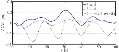
In Fig. 8, we depict the system ACE, when using the online estimationb= ˆβ=−1.158pu/Hz for the 20th_{min, the AFRC}

b = β, and a fixed value b = −1.7 pu/Hz for the period of 1 min. We may see that for b = β, we obtain the best results, since it is well known that the best choice for the frequency bias factor is the AFRC [18]. We notice that b =

ˆ

β is very close to ideal case, as desired. The reason is that the estimation is very close to the AFRC. The case of b =

−1.7pu/Hz presents the biggest oscillations. We also note that for this time period the maximum absolute values of ACE for the three cases are:0.2360pu,0.1138pu, and0.3475pu, and the regulation amounts needed for each of the three cases are: 4.3079pu, 2.3425 pu, and 7.7154 pu, respectively; thus, the use of the online estimationβˆinbis a good practice.

C. 48-Machine 140-Bus Power System

Next, we demonstrate the scalability of the proposed methodology to the online estimation of the AFRC for large power systems. In particular, we examine the IEEE 48-machine test system, which consists of 140 buses and 233 lines [22]. To implement our proposed adaptive AGC scheme, we use the MATLAB-based Power Systems Toolbox (PST) [23], by adding the AGC system model in (12)-(13). The AGC signal is allocated to the generators with a ratio proportional to their inertia constant.

We use the algorithm proposed in (45) to estimate the AFRC and use it in the calculation of the ACE. We modify the system load in a similar way as in the 9-bus 3-machine system. In Fig. 9, the ACE is plotted for the period of 1 minute by using: the estimated AFRC b = ˆβ = −5278 MW/Hz, the ARFC

b=β =−5475MW/Hz, and the valueb=−15833MW/Hz in its calculation. One can see that the proposed method yields good results and the ACE is close to zero. In addition, the maximum deviation of ACE is4.91pu,4.30pu, and14.25pu, respectively.

0 10 20 30 40 50 60

-20 -15 -10 -5 0

A

C

E

[p

u

]

t[s]

b_{= ˆ}β

b₌β

[image:9.612.337.527.639.727.2]

b_{=−15833MW/Hz}

[image:9.612.73.266.641.727.2]

VI. CONCLUDINGREMARKS ANDFUTUREWORK

In this paper, we developed simplified models that describe synchronous generator and BA area dynamic behavior. More specifically, we proposed a reduced-order generator model that is simpler than the 9-state model and approximates the synchronous generator dynamics in satisfactory levels, pro-vides better accuracy compared to the classical models, and has lower computational burden compared to other reduction models. Subsequently, we used the reduced-order model to derive a set of differential equations that describe the BA area dynamic behavior. We demonstrated in the numerical results section that these models provide a good approximation of the system state compared to the 9-state model, which is considered as the reference.

Moreover, to demonstrate the suitability of the proposed models to power system analysis, we chose to use the simpli-fied model for a BA area to design an adaptive AGC system. To this end, we express the AFRC as a function of the BA area variables that we have measurements of. Then, we used the SEWBLS algorithm to estimate the AFRC and modify the control gain of the AGC system. We showed that the use of the AFRC provides better results in the frequency regulation, in terms of the magnitude of the oscillations, the time the frequency converges to the nominal value, and the regulation amount needed. Furthermore, we showed that the proposed method gives a good approximation of the AFRC.

For the future work, we plan on validating the proposed adaptive AGC system in a real system, and compare the results against the NERC frequency response requirements. Then, we will investigate if a BA area that exercises the proposed adaptive control meets the frequency criteria, such as CPS1, CPS2, and BAAL (e.g., [24], [25]).

REFERENCES

[1] J. H. Etoet al., “Use of frequency response metrics to assess the planning and operating requirements for reliable integration of variable renewable generation,” Ernest Orlando Lawrence Berkeley National Laboratory, Tech. Rep. LBNL-4142E, December 2010.

[2] P. Kundur, N. J. Balu, and M. G. Lauby, Power System Stability and Control, ser. Discussion Paper Series. McGraw-Hill Education, 1994. [3] I. J. Perez-Arriaga, G. C. Verghese, and F. C. Schweppe, “Selective modal analysis with applications to electric power systems, Part I: Heuristic introduction,” IEEE Transactions on Power Apparatus and Systems, vol. PAS-101, no. 9, pp. 3117–3125, September 1982. [4] A. Wood and B. Wollenberg,Power Generation, Operation and Control.

New York: Wiley, 1996.

[5] J. Jiang and Y. Zhang, “A revisit to block and recursive least squares for parameter estimation,”Computers & Electrical Engineering, vol. 30, no. 5, pp. 403–416, 2004.

[6] E. J. Davison, “A method for simplifying linear dynamic systems,”IEEE Transactions on Automatic Control, vol. 11, no. 1, pp. 93–101, January 1966.

[7] N. Jaleeli, L. S. VanSlyck, D. N. Ewart, L. H. Fink, and A. G. Hoffmann, “Understanding automatic generation control,” IEEE Transactions on Power Systems, vol. 7, no. 3, pp. 1106–1122, August 1992.

[8] M. Scherer, E. Iggland, A. Ritter, and G. Andersson, “Improved fre-quency bias factor sizing for non-interactive control,” inProc. of Cigre Session 44, Paris, France, August 2012.

[9] D. Chen, S. Kumar, M. York, and L. Wang, “Smart automatic generation control,” inProc. of IEEE Power and Energy Society General Meeting, July 2012, pp. 1–7.

[10] J. Nanda, S. Mishra, and L. C. Saikia, “Maiden application of bacterical foraging-based optimization technique in multiarea automatic generation control,”IEEE Transactions on Power Systems, vol. 24, no. 2, pp. 602– 609, May 2009.

[11] T. Yu, B. Zhou, K. W. Chan, and B. Yang, “Stochastic optimal relaxed automatic generation control in non-Markov environment based on multi-step Q(λ) learning,”IEEE Transactions on Power Systems, vol. 26, no. 3, pp. 1272–1282, Aug. 2011.

[12] C. Concordia and L. K. Kirchmayer, “Tie-line power and frequency control of electric power systems,”Power Apparatus and Systems, Part III. Transactions of the American Institute of Electrical Engineers, vol. 72, no. 2, Jan. 1953.

[13] Standard bal-003-1, frequency response and frequency bias setting. [Online]. Available: www.nerc.com

[14] P. W. Sauer and M. A. Pai,Power System Dynamics and Stability. Upper Saddle River, NJ: Prentice Hall, 1998.

[15] L. Wang and D. Chen, “Extended term dynamic simulation for AGC with smart grids,” inProc. of IEEE Power and Energy Society General Meeting, July 2011, pp. 1–7.

[16] D. Apostolopoulou, P. W. Sauer, and A. D. Dom´ınguez-Garc´ıa, “Auto-matic generation control and its implementation in real time,” inProc. of Hawaii International Conference on System Sciences (HICSS), January 2014, pp. 2444–2452.

[17] I. J. Perez-Arriaga, “Selective modal analysis with applications to electric power systems,” Ph.D. dissertation, Massachusetts Institute of Technology, Cambridge, MA, June 1981.

[18] C. D. Vournas, E. N. Dialynas, N. Hatziargyriou, A. V. Machias, J. L. Souflis, and B. C. Papadias, “A flexible AGC algorithm for the Hellenic interconnected system,”IEEE Transactions on Power Systems, vol. 4, no. 1, pp. 61–68, February 1989.

[19] D. Apostolopoulou, A. D. Dom´ınguez-Garc´ıa, and P. W. Sauer, “Online estimation of power system actual frequency response characteristic,” in Proc. of IEEE Power and Energy Society General Meeting, July 2014, pp. 1–4.

[20] Powerworld simulator version 16, user’s guide. [Online]. Available: www.powerworld.com

[21] M. Perninge, M. Amelin, and V. Knazkins, “Load modeling using the Ornstein-Uhlenbeck process,” inProc. of IEEE International Power and Energy Conference, December 2008, pp. 819–821.

[22] Power system test case archive, University of Washington. [Online]. Available: http://www.ee.washington.edu/research/ pstca/

[23] Power system toolbox. [Online]. Available: http://www.eps.ee.kth.se/personal/vanfretti/pst

[24] Real power balancing control performance, BAL-001-1. [Online]. Available: http://www.nerc.com

[25] Real power balancing control performance, BAL-001-2. [Online]. Available: http://www.nerc.com

Dimitra Apostolopoulou was awarded a Ph.D. and a M.S. in Electrical and Computer Engineering from University of Illinois at Urbana-Champaign in 2014 and 2011, respectively. She received her undergraduate degree in Electrical and Computer Engineering from National Technical University of Athens, Greece in 2009. She currently works in the Smart Grid and Technology Department at Commonwealth Edison Company. Priorly, she was a Postdoctoral Research Associate at University of Illinois at Urbana-Champaign. Her research interests include power system operations and control, market design and economics.

Alejandro D. Dom´ınguez-Garc´ıa received the degree of “Ingeniero Indus-trial” from the University of Oviedo (Spain) in 2001 and the Ph.D. degree in electrical engineering and computer science from the Massachusetts Institute of Technology, Cambridge, MA, in 2007.

He is an Associate Professor in the Electrical and Computer Engineering Department at the University of Illinois at Urbana-Champaign, where he is affiliated with the Power and Energy Systems area; he also has been a Grainger Associate since August 2011. He is also an Associate Research Professor in the Coordinated Science Laboratory and in the Information Trust Institute, both at the University of Illinois at Urbana-Champaign.

Dr. Dom´ınguez-Garc´ıa received the National Science Foundation CAREER Award in 2010, and the Young Engineer Award from the IEEE Power and Energy Society in 2012. In 2014, he was invited by the National Academy of Engineering to attend the U.S. Frontiers of Engineering Symposium, and selected by the University of Illinois at Urbana-Champaign Provost to receive a Distinguished Promotion Award. In 2015, he received the U of I College of Engineering Dean’s Award for Excellence in Research.

He is an editor of the IEEE TRANSACTIONS ON POWER SYSTEMS and the IEEE POWER ENGINEERING LETTERS.