Improving RF-based partial discharge localization via machine learning ensemble method



Abstract— Partial discharge (PD) is regarded as a precursor to plant failure and therefore an effective indication of plant condition. Locating the source of PD before failure is key to efficient maintenance and improving reliability of power systems. This paper presents a low cost, autonomous partial discharge radiolocation mechanism to improve PD localization precision. The proposed radio frequency based technique uses the Wavelet Packet Transform (WPT) and machine learning ensemble methods to locate PDs. More specifically, the received signals are decomposed by the WPT and analyzed in order to identify localized PD signal patterns in the presence of noise. The Regression Tree algorithm, Bootstrap Aggregating method and Regression Random Forest (RRF) are used to develop PD localization models based on the WPT-based PD features. The proposed PD localization scheme has been found to successfully locate PD with negligible error. Additionally, the principle of the PD location scheme has been validated using a separate test dataset. Numerical results demonstrate that the WPT-Random Forest PD localization scheme produced superior performance as a result of its robustness against noise.

Index Terms— Partial discharge, Localization, Wavelet packet transform, Bootstrap aggregating, Random forest, Regression tree.

I. INTRODUCTION

The presence of partial discharge in electrical assets is indicative of some defect in the insulation system of the device. These discharges can harm the insulation and might lead to total breakdown of the asset over time with social and economic consequences. The uninterrupted monitoring of these assets is therefore paramount in the operation of the electric power system. One of the leading candidates for effective condition monitoring of electrical assets is partial discharge [1] [2] PDs are ionization processes that occur in void filled gases or liquids inside insulation, in dielectric surfaces, and in the proximity of sharp metallic objects [3] [4] [5] . PDs emit part of the energy they produce as electromagnetic waves [6] and this has motivated the use of radio sensors for detection and localization

Manuscript received June 29, 2018; revised December 21, 2018; revised February 11, 2019; accepted March 17, 2019. This work was supported by the Engineering and Physical Sciences Research Council grant EP/J015873/1 and Tertiary Education Trust Fund (TETFund) Nigeria.

E. Iorkyase, C. Tachtatzis and R. C. Atkinson are with the Department of Electronic and Electrical Engineering, University of Strathclyde, Glasgow,

of the discharge sources. Early detection of PD reduces the risks of harm to insulation and can prevent sudden breakdown. Once the occurrence of PD has been established, it is a matter of urgency to locate the discharge source as quickly and accurately as possible to enable corrective maintenance operation when the maintenance activity is most cost effective and before the equipment loses performance or suffers catastrophic failure.

RF-based PD location has been widely studied [7] [8] [9] [10] [11]. Given a model of radio signal propagation in a particular environment, the TDoA, AoA and/or RSS [5] [12] [13] [14] [15] algorithm can be used to estimate the distance from a source to a receiver and thereby trilaterate the location of the PD. UHF antenna arrays [8] have also been used to locate impulsive PDs in a substation. In cables, time-domain reflectometry (TDR) [16] which is based on the time difference of arrival is used to locate the source of PD along a cable. The time-difference-of-arrival (TDoA) of the received signals is established by cross-correlation and the location of PD is found by multi-lateration [17]. Unfortunately, this technique is uneconomical and complex requiring accurate synchronization, and Line-of-Sight (LOS) propagation for accurate location estimation. It also requires a detailed RF propagation model for every environment in which this system is deployed and this is not trivial to obtain. The environment in which PD is expected is characterized by interference, multipath propagation and presence of metallic obstacles leading to a complex spatial radio environment, which is difficult to describe by ready-made models.

In previous work, we have adopted a pattern matching technique which uses features of the received radio signals to infer PD location [14]. The pattern matching technique can be regarded as a low cost technique compared to those based on time estimation [18]. It turns the frequency-selective multipath phenomenon to surprisingly good use: by combining the multipath pattern with other PD pulse characteristics, it creates unique RF signatures representing different locations.

In this study, we propose to deploy a spatial array of low cost off-the-shelf commercial radio sensors in form of wireless

Scotland, UK, G1 1XW (e-mail: [email protected], [email protected], [email protected]).

I. A. Glover, P. Lazaridis, D. Upton, B. Saeed are with the Department of Engineering and Technology, University of Huddersfield, Queensgate, Huddersfield, HD1 3DH (e-mail: [email protected], [email protected], [email protected], [email protected])

Improving RF-based Partial Discharge

Localization via Machine Learning Ensemble

Method

sensor network in an electricity substation. The proposed solution allows a PD monitoring system to be permanently deployed and thus monitor the substation uninterrupted in real-time and at low cost. In this approach, the network autonomously creates a spatial map of the RF characteristics of the radio signals and uses sophisticated machine learning techniques to estimate the location of PD sources. In previous work we have used machine learning algorithms to build a bespoke propagation model for the radio environment from the perspective of each node [13]. Based on the relative received signal strength of a PD pulse at each node, a multilateration approach can be deployed to infer PD location. In this work, we go further by investigating the temporal signatures of the received pulses to determine if they able to provide a more accurate estimation of location than raw energies alone.

One approach, we have considered, in engineering PD features for source localization is direct extraction from measured time domain PD signals. These features infer the location where PD originate and are referred to as location dependent parameters. Features extracted from time domain signals for PD location assume a single PD type scenario. However, localization of PD using such features may not be sufficient in real electricity substations where different types of PD occur. Therefore, we adopt a modified version of this approach by examining the time-domain signatures from each pulse, but in multiple distinct frequency bands. This technique adds another discriminatory dimension to the problem and yields superior results. In the frequency domain, PDs of different types can be effectively characterized for localization. Most of the frequency domain methods used in PD signal analysis and localization are based on the well-known Fast Fourier transform (FFT) techniques [16] [19]. However, PD signals are stochastic and often demonstrate a nonstationary and transient nature, carrying small yet informative components embedded in larger repetitive signals [1]. This limits the application of FFT based techniques for PD localization. In this work, a low cost approach, which uses the Wavelet Transform [20] to decompose RF PD signals into different frequency bands and extract PD location dependent parameters for robust PD localization is presented and evaluated in this paper. A machine learning ensemble technique is employed for improved PD localization.

II. FEATURE EXTRACTION

Feature extraction is one of the necessary preprocessing steps of machine learning and pattern matching [21]. Its aim is to extract the most informative inputs (features) from raw PD signals. Good features are highly correlated with the expected outputs but have low correlation with each other. The extracted features facilitate the subsequent learning and generalization steps, and in some cases, lead to better interpretations.

Partial discharge (PD) RF pulses collected during the measurement campaign are corrupted by noise due to external disturbances. Extracting PD pulses from such noisy measurements is therefore crucial. It is also important that this is done in such a way that the features of the PD pulse are

preserved as much as possible. In this work, a multivariate de-noising method [22] [23] [24] that combines wavelets and Principal Component Analysis (PCA) is applied to the PD data in order to isolate the PD signals from noise without assuming any a priori knowledge of the PD features. This technique combines the decomposition of information given by the wavelet transform with the ability to orthogonalize variables provided by PCA. The objective is to obtain de-noised PD data so as to extract meaningful information for PD location. Samples of noise corrupted PD signals recorded are as shown in Fig. 1. PCA here is not used to discover new variables which could be of interest, but to take advantage of the deterministic links among the signals, offering an additional de-noising layer by omitting insignificant principal components. In parallel, PCA is performed on the wavelet approximation coefficients to keep the most important features of the PD signals. Kaiser's rule [25] is used to automatically select the minimum numbers of retained principal components (components associated with eigenvalues exceeding the mean of all eigenvalues). The Daubechies wavelet db14 with a 5th level decomposition which has been used for PD de-noising [26] is adopted in this work. Owing to the fact that only a few of the wavelet coefficients describing PD waveform carry significant information, hard-thresholding is employed. The PD de-noised signal samples are shown in Fig. 2.

(a) Pulse 1 – Position 1

(c) Pulse 3 – Position 2

(d) Pulse 4 – Position 2 Fig. 1. Emulated PD pulse with noise

A. Wavelet Transform

The application of wavelet transformation in PD signal analysis is a well-known technique which overcomes the problems of other signal processing techniques such as the Fourier Transform which can describe the frequency components contained within a complex signal, but cannot indicate where in time those frequencies reside. A wavelet-based approach permits isolation and extraction of energies in both time and frequency. In any complex radio environment, such as a substation, multipath propagation will occur as a result of reflection and diffraction from various obstacles and structures; this gives rise to many delayed and attenuated versions of the emitted PD pulse. The superposition of these received pulses produces a temporal signature (energy versus time) from which higher order features can be extracted. The shape of the pulse in the time-domain will be dependent on the location of the source. Multipath effects are also known to be frequency-selective in that the shape of the signature will change based on the frequency of the pulse. Thus, the aggregated PD pulse as seen by the receiver can be effectively band-pass filtered to produce distinct time-energy signatures in each band. In doing so, we can exploit the frequency-selective nature of multipath propagation to generate more distinct features to aid the localization algorithm. This filtering process is achieved via a wavelet-based approach as follows.

(a) Pulse 1 – Position 1

(b) Pulse 2 – Position 1

(c) Pulse 3 – Position 2

(d) Pulse 4 – Position 2 Fig. 2. De-noised PD pulses

Unlike spectral analysis that represents a signal as a sum of sinusoidal functions, the wavelet transform decomposes the signal into wavelets of various scales in the time-domain with variable window sizes thus revealing the local structure in the time-frequency domain. The continuous wavelet transform [27] of a signal 𝑠(𝑡), is given as:

where 𝜓(𝑡) is the mother wavelet, 𝑎 and 𝑏 are the scale and shift parameters respectively. The computational burden involved in computing the many coefficients generated by continuous wavelet transform for every scale and time is overwhelming. An efficient alternative is to discretize 𝑎 and 𝑏 by replacing 𝑎 = 2−𝑗 and 𝑏 = 𝑘2−𝑗, where 𝑘 and 𝑗 are integers. This forms the discrete version of wavelet transform. This is expressed as:

𝑊𝑠(𝑗, 𝑘) = ∫ 𝑠(𝑡)2𝑗 2⁄ _𝜓

𝑗,𝑘∗ (2𝑗𝑡 − 𝑘)𝑑𝑡 +∞

−∞ , (2)

The Discrete Wavelet Transform (DWT), which is one of the popular methods in the wavelet transformation family has been widely used in PD signal processing, classification and de-noising [20] [28] [29] [30] [31]. The DWT uses a cascade of low and high pass filters to decompose the PD signal into two components: detail coefficients (DCs), which contain the high frequency, low scale information of the PD signal and approximation coefficients (ACs), which capture the low frequency, high scale information of the PD signal. While the DCs remain unchanged at each level of decomposition, the ACs are further decomposed into DC and AC subsets. This process continues until the final decomposition level [32]. In this way, DWT decomposes PD signals into different scales, generating multi-scale features which reveal the local features of the PD signals. However, with DWT some intrinsic characteristics of the signals in the high frequency region are still buried in the DCs since only ACs are decomposed in each level.

B. Wavelet Packet Transform

The Wavelet Packet Transform (WPT) [33] [34] [35] is viewed as an extension of the DWT providing a level by level transformation of a signal from the time domain to the frequency domain. The top or first level of the WPT is the time representation of the PD signal. At every other level down the WP decomposition tree, there is a decrease in temporal resolution and a corresponding increase in frequency resolution. This helps capture the high frequency information in the PD signals which are not normally represented in DWT.

Fig. 3. General architecture of the WPT

In other words, unlike the DWT, the WPT decomposes both the DCs and the ACs simultaneously at every level. Therefore, the WPT has the same frequency bandwidth in each resolution. This enables the WPT to preserve the information in the original PD signals, resulting in robust features. The general architecture of the WPT decomposition is shown in Fig. 3. The tree is typically a binary tree, where each node has both DCs (right sub-node) and ACs (left sub-node). In practice, WPT decomposition is achieved via a quadrature mirror filter pair (low-pass and high-pass). Let the wavelet packet function be given by:

𝑉𝑗,𝑘𝑛(t) = 2j/2Vn(2jt − k) (3)

where 𝑗 is a scaling parameter, 𝑘 and 𝑛 are a translation and oscillation parameters respectively. And the scaling and wavelet function represented by𝜙(𝑡) and 𝜓(𝑡) respectively, then the wavelet filters can be constructed using the following expression [36]:

𝜙(𝑡) = √2 ∑ 𝑔𝑙𝜙(2𝑡 − 𝑘)𝑘 (4) 𝜓(𝑡) = √2 ∑ 𝑔ℎ𝑘 𝜙(2𝑡 − 𝑘) (5)

where 𝑔𝑙 and 𝑔ℎ are the low-pass and the high-pass filters respectively. The scaling and wavelet functions are equivalent to the first two wavelet packet functions given as:

𝑉0,0 0 (𝑡) = 𝜙(𝑡) (6) 𝑉0,0 1 (𝑡) = 𝜓(𝑡) (7)

This implies that for 𝑛 = 0,1,2, …., the wavelet packet functions can be expressed as:

𝑉𝑗,𝑘2𝑛(𝑡) = √2 ∑ 𝑔𝑙𝑉𝑘 𝑗−1,𝑘𝑛 (2𝑡 − 𝑘) (8)

𝑉𝑗,𝑘2𝑛+1(𝑡) = √2 ∑ 𝑔ℎ𝑉𝑘 𝑗−1,𝑘𝑛 (2𝑡 − 𝑘) (9)

Therefore, features can be extracted from both DCs and ACs at different levels to obtain valuable information. In [37], the WPT was used to decompose PD signals into multiple scales, and extract PD features for PD classification. In this work, WPT is used for locating PD sources.

C. Feature Extraction of PD Signals using WPT

level is set to 4 since the signal is long. The 4-level WPT decomposition generates a tree with 16 terminal nodes, corresponding to the frequency sub-bands. Features are defined based on the wavelet packet node coefficients. For any function 𝑓, the wavelet packet coefficient is given by:

𝑣𝑗,𝑛,𝑘(𝑡) = 〈𝑓, 𝑉𝑗,𝑘𝑛〉 = 〈𝑓, 2𝑗 2⁄ 𝑉𝑛(2𝑗)〉 (10) Each 𝑣𝑗,𝑛,𝑘 coefficient measures a specific sub-band frequency content, controlled by the scaling parameter j and the oscillation parameter 𝑛, of a signal around the time instant 2𝑗_{𝑡. Unlike} discrete wavelet transform, the filtering operations in wavelet packet transform, are also applied to the wavelet, or detail coefficients. The frequency-localised filter; Fejer-Korovkin wavelet has been shown to be a good approximation [38]. The result is that wavelet packets provide a sub-band filtering of the input signal into progressively finer equal-width intervals. At each level 𝑗, the frequency axis is divided into 2𝑗 _sub-bands. The sub-bands in Hertz at level 𝑗 are approximately

[𝑛𝑓𝑠 2𝑗+1,

(𝑛+1)𝑓𝑠

2𝑗+1 ) (11)

where 𝑛 = 0,1, … , 2𝑗_{− 1 and 𝑓𝑠 is the sampling frequency.}

(a)

(b)

(c)

(d)

Fig. 4. PD wavelet packet node energy distribution for the 4 de-noised pulses in Fig. 2 (a) pulse 1-position 1 (b) pulse

2-position 1 (c) pulse 3-2-position 2 (d) pulse 4-2-position 2

(a)

(b)

Fig. 5. Normalized signal energy by node for (a) signals in Fig. 4a/b, and (b) signals in Fig. 4c/d.

The wavelet packets have the added benefit of being an orthogonal transform, which means the energy in the signal is preserved and partitioned among the sub-bands as mentioned earlier. Therefore, the wavelet packet node energy can represent the characteristics of PD signals, and it is defined as

Section III. Specifically, Fig. 4 a/b depicts the energy profile of two distinct pulses transmitted from the same location (location 1), and Fig. 4 c/d depicts the energy profile of another two pulses transmitted from a second location (location 2). By examination of packet nodes 1 to 3 (first three bars in Fig. 4), it is evident that subplots a and b are very similar, these are distinct signals from the same location. Likewise, subplots c and d are very similar, these represent two distinct pulses from a second location. However, the signals from a or b are distinct from those of c or d. Thus, the wavelet packet node energy distribution represents an excellent set of features for PD localization because it is (i) time invariant, and (ii) location dependent. It is important to identify the frequency bands that contain most of the PD pulse energy. PD signals are known to have a very short duration (nanosecond), which implies a high frequency content. However, there are always dominant frequency bands that contain greater pulse energy in the entire spectrum. The relative energy by node shown in Fig. 5 reveals the nodes with higher percentage of pulse energy, indicating 3 frequency passbands of interest. The resulting passbands emphasize frequencies between 62.5 – 250 MHz, which contains large portions of the PD signal energy. The lower and upper frequencies of each wavelet packet frequency band are presented in Table 1. In the presence of noise the PD energy will be buried in noise in some frequency bands making it a challenge to find where PDs lie. The significant advantage of the proposed WPT technique lies in its ability to identify these frequency bands even in noisy PD signals. Given noisy PD signals as shown in Fig. 1, it has been demonstrated that the wavelet packet transform identifies the frequency bands with most of the PD pulse energy as wavelet packet nodes at the terminal level using (12). The energy distribution of these noisy signals in the frequency bands after transformation is as shown in Fig. 6. This demonstrates the robustness of the proposed technique in the presence of noise. In this work, each node energy equivalent to energy in a frequency passband, represents an individual PD feature component.

Table 1.WPT-based extracted PD frequency bands

Lower frequency Upper frequency

BAND 1 62.5 MHz 125 MHz

BAND 2 125 MHz 187.5 MHz

BAND 3 187.5 MHz 250 MHz

This work is based on the assumption that all PD features extracted using the WPT provide meaningful information for inferring the PD location. To demonstrate that this is a reasonable assumption, Fig. 7 (a-c) shows how the maps of the PD features at each of the 3 antennas vary with location. The effect of multipath and signal distortions add to the unique signature created at different locations.

(a)

(b)

(C)

(d)

Fig. 6. PD wavelet packet node energy distribution for the 4 noisy pulses in Fig. 1 (a) pulse 1-position1 (b) pulse

2-position1 (c) pulse 3-position 2 (d) pulse 4-position 2.

(b)

(c)

Fig. 7.Spatial representation of WPT-based PD energy in band 1.

III. EXPERIMENTAL PROCEDURE

In order to evaluate the feasibility of using the WPT-based frequency domain PD features in conjunction with machine learning ensembles to locate a PD source, an experiment was conducted in the laboratory at the University of Strathclyde with approximate dimensions of 19.2m x 8.4m. This environment is characterized by multipath propagation which is a result of cluttered objects including metallic ones. Although the radio environment within the laboratory cannot be expected to approximate that within an electrical substation, it is sufficiently complex to enable evaluation of the PD localisation techniques being investigated. The floor map is shown in Fig. 8. On the map, three receiver sensors indicated by antennas are positioned at random with considerable distance between them whereas reference (training) and test locations represented as (blue) circles and (red) diamond marks respectively are defined on a grid. These training and test locations simulate PD sources and are so called given that they represent different sets of data to be used in this work. At every training and test location, PD emulated signals are generated and recorded. A pulse signal generator was used to emulate PD signals in this experiment. The pulse generator is capable of generating sub-nanosecond current pulse which was fed to a monopole antenna. The radiating monopole antenna therefore represents an artificial PD source. Commercial-off-the-shelf Omni-directional antennas operating at 173MHz were used to capture the generated PD signals. The frequency response of the antennas is depicted in Fig. 9.

Fig. 8. PD measurement grid

Fig. 9. Antenna frequency response

These sensors were connected to a multichannel digital oscilloscope where the PD pulse traces were recorded for further analysis. 20 samples of PD signals were generated and collected for each of the 144 reference (training) locations (blue circles) to build a training database. The training points were separated by 1m on a uniform grid. For testing the PD localization scheme developed in this paper, 20 PD signal measurements were collected at each of the 32 distinct test locations (red diamonds) on the same grid in Fig. 8. The spacing between the test points is 2.5m. This setup ensures that the 20x144 training and 20x32 testing samples are disjoint enough to provide realistic results. A sample of the PD emulated pulse and the received pulse captured by the sensors is as shown in Fig. 10.

IV. MACHINE LEARNING-BASED PDLOCALIZATION

METHODS

A. Regression Tree-Based PD Localization Method

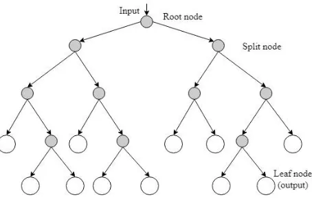
The Regression Tree is one of the most efficient machine learning algorithms used for predictions [39] [40] [41]. It is considered a variant of a binary decision tree model composed of linear regression functions at the leaf nodes. In this work, it is designed to learn and approximate the nonlinear function (PD locations/WPT-based PD features) by piecewise linear functions at the leaf nodes. In other words, the nonlinear mapping of PD features to PD location coordinates is handled by splitting the problem into a set of smaller problems addressed with simple linear predictors. Fig. 11 shows the architecture of a regression tree. Each node in the tree is designed to split the data so as to form clusters where accurate predictions can be performed with simple models. During training, a PD regression tree model is built top-down from the root node through binary recursive partitioning, which is an iterative process that splits the PD training data (PD features/location) into subsets that contain features with similar values. The parameters of the tree such as number of splits are optimized during training. A sum of squares reduction criterion is used in partitioning the data.

Fig. 11. General architecture of a regression tree.

The algorithm selects the split at each node that minimizes; 𝑆𝑆 = ∑ ((𝑥, 𝑦)𝑖− (𝑥, 𝑦)𝑅)2

𝑅 + ∑ ((𝑥, 𝑦)𝑖𝐿 − (𝑥, 𝑦)𝐿)2 (13)

where (𝑥, 𝑦)R and (𝑥, 𝑦)L are the estimated values for the right and left nodes respectively. This process continues until it reaches the terminal (leaf) node. The terminal nodes of the tree which represents a cell of the partition, store the models that approximate the best desired output. Suppose the training points at the terminal node are (𝑟_𝑖, (𝑥, 𝑦)_𝑖), (𝑟₂, (𝑥, 𝑦)_𝑖), . . . (𝑟𝑛, (𝑥, 𝑦)𝑛), then the local model for the terminal node is

(𝑥̂, 𝑦̂) =1_𝑛∑𝑛𝑖=1(𝑥, 𝑦)𝑖 (14)

In the localization phase, the location coordinate of any PD

sample (features) can be estimated by following through the branches of the obtained tree model. Despite the simplicity that comes with the implementation of regression trees, the issue of overfitting affects its performance. When fully grown, it may lose some generalization capability.

B. Bootstrap Aggregating Method for PD Localization Bootstrap aggregating [42] [43] [44], also known as bagging is a machine learning ensemble algorithm that combines a multitude of decision trees in order to improve performance. For PD localization, bagging is used to model the non-linear relationship between WPT-PD features and PD location. Instead of growing a single tree from the complete data set during training, bagging grows many trees using bootstrap (equiprobable sampling with replacement) samples of the PD data. Each sample is different from the original data set, yet resembles it in distribution and variability as a result of random sampling. Different tree models are grown for each bootstrap sample. Mathematically, given a training input set 𝑅 = 𝑟1,… ,𝑟𝑛 and corresponding training output set (𝑋, 𝑌) = (𝑥, 𝑦)_{𝑖,… ,}(𝑥, 𝑦)𝑛, bagging repeatedly (M times) selects subsets (randomly sample with replacement) of these training set and builds trees with each subset. For 𝑚 = 1, … . , 𝑀: bagging builds 𝑡𝑚 models. After training, the location estimate for unseen sample 𝑟′ can be taken as the average estimates of all the individual tree models on 𝑟′ _{given as;}

𝑡̂ =_𝑀1∑𝑀 𝑡𝑚(𝑟′₎

𝑚=1 (15) The performance of bagging is affected by the particular bootstrap sample size used. Therefore, Bayesian optimization is used to tune the model parameters. PD location is then determined by taking the average of the outputs from all the trees. Random sampling helps overcome the problem of overfitting in regression trees and improves predictions. However, there exist high correlations in prediction among some of the PD localization subtrees, limiting the performance of the bagging regression trees. This motivates the use of a

robust PD localization algorithm: random forest.

C. Random Regression Forest PD Localization Method Random Regression Forest (RRF) is an ensemble of different regression trees widely used in prediction [45] [46] [47]. The main idea of RRF is to grow many regression trees based on some randomly selected features (sub-spacing) from randomly selected samples with bootstrap strategy. In the context of PD localization, each tree is regarded as a function approximation problem consisting of a non-linear mapping of the PD input features onto the x-y coordinates representing PD location. The nonlinearity is achieved by dividing up the original PD localization problem into smaller ones, solvable with simple models. A multivariate RRF model is developed to locate PD source to its x and y coordinate.

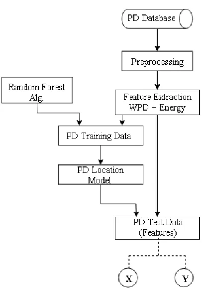
Fig. 12. Flowchart for Random Forest PD Localization The RRF-PD localization technique consists of two phases: a training phase and a location estimation phase. In the training phase, RRF grows multiple regression trees from bootstrap samples of the training data. Each sample subset comprises PD features and associated ground-truth locations. At each split or node, only a random subset of the PD features is considered. The size of the forest is fixed and all the trees are trained in parallel. During training, the parameters of the model are optimized.

In the location estimation phase, each previously unseen PD features sample is given as an input to each tree in the forest starting at the root and the corresponding sequence of tests applied. Each tree gives an estimate of the location coordinate and the final prediction is taken as the average of the trees predictions. The flowchart of the RRF framework is as shown in Fig. 12. The selection of random samples of features at each split produces uncorrelated subtree predictions. Combining multiple decorrelated PD-tree models increases robustness to variance and reduces overall sensitivity to noise. This is demonstrated by the results obtained.

V. LOCALIZATION RESULTS AND DISCUSSION

This section provides empirical evaluation of the performance of the PD localization methods described in section 3. The PD data used for testing is taken from a set of 32 different grid locations, independent of the training set, but obtained with the same procedure.

A. Evaluating Localization Accuracy

Localization errors for each PD location model developed are shown in Table 2. The x and y coordinate error columns represent the error in the x and y direction respectively, however, these columns may not correspond to the same physical location. For example, for RT-best the x-error is 0 for one location but has a non-zero y value. Similarly, for a different location y is 0 but has a non-zero error. Errors in x and y coordinates are defined as absolute differences between predicted and true locations. Column 3 represents the overall localization error (Euclidean distance between the predicted and true locations). Despite the data variability and the area covered, a mean error of 1.9 m obtained is sufficient for PD location. The models are trained on 2880 PD data measurements and tested on 640 PD data measurements. The normalized WPT-based features extracted from the 2880 measurements with corresponding locations are used as input to the models for training. The maximum number of PD features used at each split is 1/3 of the total number of features. In this work, 1000 trees are grown. This optimal number is estimated internally during the computations.

Table 2. Statistics of PD location error for each method

PD Location Method X-coordinate error (m)

Y-coordinate error (m)

Location Error (m) Reg. Tree (best) 0.0000 0.0000 0.5000 Reg. Tree (worst) 8.5000 6.5000 8.9253 Reg. Tree (mean) 1.3712 1.9808 2.7017 Reg. Tree (variance) 2.0257 2.8912 3.4191

Bootstrap (best) 0.0020 0.0029 0.0829 Bootstrap (worst) 5.6550 6.0736 6.2197 Bootstrap (mean) 0.9452 1.5213 1.9839 Bootstrap (variance) 0.5786 1.7839 1.6330

RRF (best) 0.0031 0.0021 0.0789

RRF (worst) 5.1260 5.7435 6.0531

RRF (mean) 1.0019 1.4296 1.9152

RRF (variance) 0.5512 1.4633 1.3930

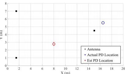
Fig. 13 shows the estimated PD source location (red diamond) with the lowest localization error for each model using WPT-based features. The blue dot represents the actual PD source position. The black squares represent emulated sensor node positions. The results show that the minimum location error is superior when ensemble methods are applied on the WPT-based features. Regression tree can locate the exact x or y coordinates with zero error in some instances as shown in Table 2 but fails to provide a robust model, with worst location error as high as 8.9 m. This is shown in Fig. 14.

regression tree. Given that the spacing between test locations is 2.5m, the proportion of test data with a localization error below this value is also evaluated. For the regression tree method, 68% of test points were below 2.5m. For the bagging algorithm, 75% are below, and for the random forest 78% are below.

(a)

(b)

(c)

Fig. 13. PD best location estimates: (a) Random Forest, (b) Bagging, (c) Regression Tree

Fig. 14. Regression Tree PD worst location estimate

(a)

(b)

(c)

Fig. 15. CDF of location errors in (a) x-coordinate (b) – coordinate (c) overall

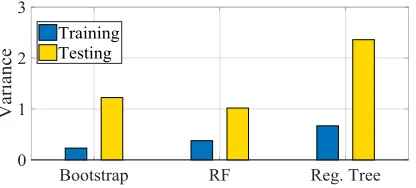
B. Evaluating model Robustness

Regression Tree indicates a less precise location estimate. This further demonstrates the robustness of the proposed WPT-based Random Forest PD localization scheme.

Fig. 16. Variance of location error

Fig. 17. PD location results for 3 different points

C. Comparison with Related Works

There are other substation-wide PD localization schemes in literature that are worth comparing with our proposed solution. In [48], the authors developed a Software Defined Radio (SDR) PD localization system based on received signal strength to infer PD location. However, they presented results for a single location estimate which we assumed to be the best location estimate; this approach yielded a location error of 1.3 m. Another RSS-based PD localization system was proposed in [49]. Here, the system involves estimating the path loss exponent and converting the RSS into distance. Two scenarios were created in terms of the number of receiving sensors used for capturing PD signals; seven sensors for scenario 1 and eight sensors for scenario 2. The test site was an 18m X 18m empty room. For the nine test locations, the best estimated location error for scenario 1 and scenario 2 are 0.78 and 1.06 m respectively. In another work [50], a PD localization scheme based on RSS fingerprint was proposed for a 24m2 _{test bed with}

grid spacing of 1m X 1m. The localization phase includes two stages of processing: a preliminary localization stage where particle swarm optimization and back propagation neural network are used, and a more accurate localization stage where compressive sensing is employed for accurate localization. Their result shows an average localization error of 0.89m with maximum error 3.61m. However, this result comes at an extra cost of two stages of computation in the localization phase. A probability based technique for PD source localization was proposed in [51]. Time difference of arrival (TDoA) was used as PD feature. A test of three PD sources was carried out and the result indicates localization errors of 0.56m, 1.59m and

0.18m for the three sources. In [52], an automated system for PD detection and localization based on Gaussian mixture model was presented. Time delay of arrival was used to locate PD sources. This work presented result for eight location estimate with minimum error of 0.5m and an average location error of 1.4m. Authors in [53] proposed an RSS-based PD localization method to locate power equipment in substation with potential insulation defect. This involves two stages of localization: a preliminary localization by cluster recognition and compressed sensing algorithm. The test site used for this experiment measured 24m X 24m with 625 grid points (1m X 1m). Their result indicates that the proportion of estimated location errors within 3m is 89.6 %. Our proposed solution, WPT-based RRF PD localization scheme is a simple and low-cost solution for PD localization with best estimated location error of 0.31 m. Our result also indicates that 91% of the PD sources were located with error less than 3 m.

VI. CONCLUSION

A robust PD localization scheme based on the wavelet packet transform and the ensemble learning method has been considered. The scheme utilizes the PD measurements captured with sensors placed in the vicinity of the discharge source, as follows.

(1) The measured PD signals are first decomposed using WPT decomposition to extract PD location dependent features. The WPT selects the frequency bands with equal bandwidth where the energy of the noisy PD signal is concentrated through a transformation such that the retained signal information is maximized in order to ensure high accuracy.

(2) The WPT-based PD features are then used to build the ensemble models.

(3) PD location is obtained via a multivariate regression forest algorithm which provides a more robust and accurate approach compared to regression tree and bootstrap aggregating methods.

In this study, regression forest increased the overall confidence probability of errors within 3 m to 91% compared to 70% achieved by regression tree; an improved accuracy of 29%. The results suggest that the proposed PD localization method described in this paper represents a practical approach to PD localization. The simplicity and robustness of the technique makes it worth considering in future implementations of the smart grid.

REFERENCES

[1] J. C. Hernandez-Mejia, J. Perkel, R. Harley, M. Begovic, R. N. Hampton, and R. Hartlein, "Determining routes for the analysis of partial discharge signals derived from the field," IEEE Trans.

on Dielectr. and Electr. Insul., vol. 15, no. 6, 2008.

[2] X. Peng, C. Zhou, D. M. Hepburn, M. D. Judd, and W. H. Siew, "Application of K-Means method to pattern recognition in on-line cable partial discharge monitoring," IEEE Trans. on

Dielectr. and Electr. Insul., vol. 20, no. 3, pp. 754--761, 2013.

simulation," IEEE Trans. on Dielectr. and Electr.l Insul., vol. 23, no. 1, pp. 451--459, 2016.

[4] J. Li, X. Han, Z. Liu, X. Yao, and Y. Li, "PD characteristics of oil-pressboard insulation under AC and DC mixed voltage,"

IEEE Trans. on Dielectr. and Electr. Insul., vol. 23, no. 1, pp.

444--450, 2016.

[5] H. Hou, G. Sheng, and X. Jiang, "Localization Algorithm for the PD Source in Substation Based on L-Shaped Antenna Array Signal Processing," IEEE Trans. on Power Delivery, vol. 30, no. 1, pp. 472-479, 2015.

[6] M. Yoshida, H. Kojima, N. Hayakawa, F. Endo, and H. Okubo, "Evaluation of UHF method for partial discharge measurement by simultaneous observation of UHF signal and current pulse waveforms," IEEE Trans. on Dielectr. and Electr. Insul., vol. 18, no. 2, pp. 425--431, 2011.

[7] M. X. Zhu, Y. B. Wang, Q. Liu, J. N. Zhang, J. B. Deng, G. J. Zhang, X. J. Shao and W. L. He, "Localization of multiple partial discharge sources in air-insulated substation using probability-based algorithm," IEEE Trans. on Dielectr. and

Electr. Insul., vol. 24, no. 1, pp. 157-166, 2017.

[8] H. H. Sinaga, B. T. Phung, and T. R. Blackburn, "Partial discharge localization in transformers using UHF detection method," IEEE Trans. on Dielectr. and Electr. Insul., vol. 19, no. 6, pp. 1891--1900, 2012.

[9] I. Portugues, P. J. Moore, and I. A. Glover, "Characterisation of radio frequency interference from high voltage electricity supply equipment,"in Antennas and Propagat., 2003.(ICAP 2003). 12th

Int. Conf. on, Exeter, UK, 2003.

[10] I. E. Portugues, P. J. Moore and P. Carder, "The use of radiometric partial discharge location equipment in distribution substations,"in 18th Int. Conf. and Exhibit. on Electr. Distrib., Turin, 2005.

[11] I. E. Portugues, P. J. Moore, I. A. Glover, C. Johnstone, R. H. McKosky, M. B. Goff, and L. Van Der Zel, "RF-based partial discharge early warning system for air-insulated substations,"

IEEE Trans. on Power Delivery , vol. 24, no. 1, pp. 20--29, 2009.

[12] F. Zeng, J. Tang, L. Huang, and W. Wang, "A semi-definite relaxation approach for partial discharge source location in transformers," IEEE Trans. on Dielectr. and Electr. Insul., vol. 22, no. 2, pp. 1097--1103, 2015.

[13] E. T. Iorkyase, C. Tachtatzis, P. Lazaridis, I. A. Glover, and R. C. Atkinson, "Radio location of partial discharge sources: a support vector regression approach," IET Sci., Meas. & Technol,

2017.

[14] E. T. Iorkyase and C. Tachtatzis and R. C. Atkinson and I. A. Glover, "Localisation of partial discharge sources using radio fingerprinting technique,"in Loughborough Antennas Propagat.

Conf. (LAPC), Loughborough, 2015.

[15] P. J. Moore, I. E. Portugues, and I. A. Glover, "Radiometric location of partial discharge sources on energized high-Voltage plant," IEEE Trans. on Power Delivery, vol. 20, no. 3, pp. 2264-2272, 2005.

[16] A. R. Mor,P. H. F. Morshuis, P. Llovera, V. Fuster, and A. Quijano, "Localization techniques of partial discharges at cable ends in off-line single-sided partial discharge cable measurements," IEEE Trans. on Dielectr. and Electr. Insul., vol. 23, no. 1, pp. 428--434, 2016.

[17] P. J. Moore, I. E. Portugues, and I. A. Glover, "Partial discharge investigation of a power transformer using wireless wideband radio-frequency measurements," IEEE Trans. on Power

Delivery, vol. 21, no. 1, pp. 528--530, 2006.

[18] L. Qiu, and R. A. Kennedy, "Radio location using pattern matching techniques in fixed wireless communication networks,"in Int. Symposium on Commun. and Informat.

Technol. , Sydney, 2007.

[19] T. Babnik, R. Aggarwal, and P. Moore, "Data mining on a transformer partial discharge data using the self-organizing map," IEEE Trans. on Dielectr. and Electr. Insul., vol. 14, no. 2, 2007.

[20] M. S. Abd Rahman, P. L. Lewin, and P. Rapisarda, "Autonomous localization of partial discharge sources within large transformer windings," IEEE Trans. on Dielectr. and

Electr. Insul., vol. 23, no. 2, pp. 1088--1098, 2016.

[21] J. K. Wong, H. A. Illias, and A. H. A. Bakar, "High noise tolerance feature extraction for partial discharge classification in XLPE cable joints," IEEE Trans. on Dielectr. and Electr. Insul.,

vol. 24, no. 1, pp. 66--74, 2017.

[22] L. Satish, B. Nazneen, "Wavelet-based denoising of partial discharge signals buried in excessive noise and interference,"

IEEE Trans. on Dielectr. and Electr. Insul., vol. 10, no. 2, pp.

354--367, 2003.

[23] D. Evagorou, A. Kyprianou, P. L. Lewin, P. L., "Feature extraction of partial discharge signals using the wavelet packet transform and classification with a probabilistic neural network," IET Sci., Meas. & Technol., vol. 4, no. 3, pp. 177--192, 10.

[24] M. Aminghafari, N. Cheze, J. Poggi, "Multivariate denoising using wavelets and principal component analysis,"

Computational Statistics & Data Analysis, vol. 50, no. 9, pp.

2381--2398, 2006.

[25] D. A. Jackson, "Stopping rules in principal components analysis: a comparison of heuristical and statistical approaches," Ecology,

vol. 74, no. 8, pp. 2204--2214, 1993.

[26] C. Petrarca, and G. Lupo, "An improved methodological approach for denoising of partial discharge data by the wavelet transform,"Progress In Electromagnetics Research, vol. 58, pp. 205--217, 2014.

[27] B. T. Phung, Z. Liu, TR. Blackburn, and RE. James, "Wavelet transform analysis of partial discharge signals," School of Electrical Engineering and Telecommunications, University of New South W ales, Australia.

[28] U. Khayam, and T. Kasnalestari, "System of wavelet transform on partial discharge signal denoising," in Int. Conf. of Industr.,

Mech., Electr., and Chemical Eng. (ICIMECE), Yogyakarta,

2016.

[29] E. C. T. Macedo, D. B. Araujo, E. G. da Costa, R. C. S. Freire, W. T. A. Lopes, I. S. M. Torres, J. M. R. de Souza Neto, S. A. Bhatti, and I. A. Glover, "Wavelet transform processing applied to partial discharge evaluation," Journal of Physics: Conf.

Series, vol. 364, no. 1, pp. 012--054, 2012.

[30] Q. Shan, S. Bhatti, I. A. Glover, R. Atkinson, I. E. Portugues, P. J. Moore, R. Rutherford, "Characteristics of impulsive noise in electricity substations," in 17th European Signal Processing

Conf., 2009 , 2009.

[31] M. Homaei, S. M. Moosavian, and H. A. Illias, "Partial Discharge Localization in Power Transformers Using Neuro-Fuzzy Technique," IEEE Trans. on Power Delivery, vol. 29, no. 5, pp. 2066-2076, 2014.

[32] T. Li, M. Zhou, "ECG classification using wavelet packet entropy and random forests," Entropy, vol. 18, no. 8, pp. 285 -300, 2016.

transform and neural network for detection of partial discharge in gas-insulated substations," IEEE Trans. on power Delivery,

vol. 20, no. 2, pp. 1363--1369, 2005.

[34] S. Anjum, S. Jayaram, A. El-Hag, and A. N. Jahromi, "Detection and classification of defects in ceramic insulators using RF antenna," IEEE Trans. on Dielectr. and Electr. Insul., vol. 24, no. 1, pp. 183--190, 2017.

[35] Z. Ye, B. Wu, and A. Sadeghian, "Current signature analysis of induction motor mechanical faults by wavelet packet decomposition," IEEE Trans. on industr. electron., vol. 50, no. 6, pp. 1217--1228, 2003.

[36] M. M. Eissa, "A novel digital directional transformer protection technique based on wavelet packet," IEEE Transactions on

Power Delivery, vol. 20, no. 3, pp. 1830--1836, 2005.

[37] J. Li, T. Jiang, R. F. Harrison, and S. Grzybowski, "Recognition of ultra high frequency partial discharge signals using multi-scale features," IEEE Trans. on Dielectr. and Electr. Insul., vol. 19, no. 4, pp. 1412--1420, 2012.

[38] M. Varanis, R. Pederiva, "The influence of the wavelet filter in the parameters extraction for signal classification: An experimental study.," in Proc. Series of the Brazilian Society of

Comput. and Applied Maths., vol. 5, no. 1, 2017.

[39] A. Swetapadma, and A. Yadav, "A Novel Decision Tree Regression-Based Fault Distance Estimation Scheme for Transmission Lines," IEEE Trans. on Power Delivery, vol. 32, no. 1, pp. 234 --245, 2017.

[40] D. Sanchez-Rodriguez, P. Hernandez-Morera, J. Quinteiro, and I. Alonso-Gonzalez, "A low complexity system based on multiple weighted decision trees for indoor localization,"

Sensors, vol. 15, no. 6, pp. 14809 -- 14829, 2015.

[41] H. Ahmadi, and R. Bouallegue, "RSSI-based localization in wireless sensor networks using Regression Tree," in Int. Wireless Commun. and Mobile Computing Conference

(IWCMC), Dubrovnik, 2015.

[42] M. M. bin Othman, A. Mohamed, and A. Hussain, "Determination of transmission reliability margin using parametric bootstrap technique," IEEE Trans. on Power

Systems, vol. 23, no. 4, pp. 1689--1700, 2008.

[43] D. Den Hertog, J. P. C. Kleijnen, and A. Y. D. Siem, "The correct Kriging variance estimated by bootstrapping," Journal

of the Operational Research Society, vol. 57, no. 4, pp.

400--409, 2006.

[44] A. K. Jain, R. C. Dubes, and C. Chen, "Bootstrap Techniques for Error Estimation," IEEE Trans. on patt. analysis and mach.

intellig., no. 5, pp. 628--633, 1987.

[45] A. Criminisi, D. Robertson, E. Konukoglu, J. Shotton, S. Pathak, S. White, and K. Siddiqui, "Regression forests for efficient anatomy detection and localization in computed tomography scans," Medical image analysis, vol. 17, no. 8, pp. 1293 --1303, 2013.

[46] X. Xie, J. Xing, N. Kong, C. Li, J. Li, and S. Zhang, "Improving Colorectal Polyp Classification Based on Physical Examination Data—An Ensemble Learning Approach," IEEE Robotics and

Automation Letters, vol. 3, no. 1, pp. 434--441, 2018.

[47] A. Kacete, J. Royan, R. Seguier, M. Collobert, and C. Soladie, "Real-time eye pupil localization using Hough regression forest," in IEEE Winter Conf. on Applications of Computer

Vision (WACV), New York, 2016.

[48] H. Mohamed, P. Lazaridis, D. Upton, U. Khan, K. Mistry, B. Saeed, P. Mather, MFQ Vieira, K. W. Barlee, DSW Atkinson and I. A. Glover, "Partial discharge localization based on

received signal strength," in 23rd Int. Conf. on Automation and

Comput. (ICAC), Huddersfield, UK, 2017.

[49] U. F. Khan, P. I. Lazaridis, H. Mohamed, R. Albarracin, Z. D. Zaharis, R. C. Atkinson, C. Tachtatzis, and I. A. Glover, "An Efficient Algorithm for Partial Discharge Localization in High-Voltage Systems Using Received Signal Strength," Sensor, vol. 18, no. 11, p. 4000, 2018.

[50] Z. Li, L. Luo, Y. Liu, G. Sheng, and X. Jiang, "UHF partial discharge localization algorithm based on compressed sensing,"

IEEE Trans. on Dielectr. and Electr. Insul., vol. 25, no. 1, pp.

21--29, 2018.

[51] M. Zhu, Y. Wang, Q. Liu, J. Zhang, J. Deng, G. Zhang, X. Shao, and W. He, "Localization of multiple partial discharge sources in air-insulated substation using probability-based algorithm,"

IEEE Trans. on Dielectr. and Electr. Insul., vol. 24, no. 1, pp.

157--166, 2017.

[52] D. K. Mishra, B. Sarkar, C. Koley, and NK. Roy, "An unsupervised Gaussian mixer model for detection and localization of partial discharge sources using RF sensors,"

IEEE Trans. on Dielectr. and Electr. Insul., vol. 24, no. 4, pp.

2589--2598, 2017.