Reconstructing Electrocardiogram Leads From a Reduced Lead Set Through the Use of Patient-Specific Transforms and Independent Component Analysis

Theses

Thesis/Dissertation Collections

2-10-2014

Reconstructing Electrocardiogram Leads From a

Reduced Lead Set Through the Use of

Patient-Specific Transforms and Independent Component

Analysis

Michael H. Ostertag

Follow this and additional works at:

http://scholarworks.rit.edu/theses

This Thesis is brought to you for free and open access by the Thesis/Dissertation Collections at RIT Scholar Works. It has been accepted for inclusion in Theses by an authorized administrator of RIT Scholar Works. For more information, please [email protected].

Recommended Citation

by

Michael H. Ostertag

A Thesis Submitted

in

Partial Fulfillment

of the

Requirements for the Degree of

MASTER OF SCIENCE

in

Electrical Engineering

Approved by:

_________________________________________________ (Gill R. Tsouri, Ph.D. – Advisor)

_________________________________________________ (Daniel B. Phillips, Ph.D. – Committee Member)

__________________________________________________ (Sohail A. Dianat, Ph.D. – Committee Member/Department Head)

ELECTRICAL AND MICROELECTRONIC ENGINEERING DEPARTMENT

KATE GLEASON COLLEGE OF ENGINEERING

ROCHESTER INSTITUTE OF TECHNOLOGY

ROCHESTER, NEW YORK

I would like to give special thanks to my advisor, Dr. Gill

Tsouri, who believed and supported me throughout the

prolonged process. I would also like to thank my loving family,

caring friends, and benevolent muses. All of you played a part in

helping me get where I am today.

ABSTRACT

In this exploration into electrocardiogram (ECG) lead reconstruction, two algorithms

were developed and tested on a public database and in real-time on patients. These algorithms

were based on independent component analysis (ICA). ICA was a promising method due to its

implications for spatial independence of lead placement and its adaptive nature to changing

orientation of the heart in relation to the electrodes.

The first algorithm was used to reconstruct missing precordial leads, which has two key

applications. The first is correcting precordial lead measurements in a standard 12-lead

configuration. If an irregular signal or high level of noise is detected on a precordial lead, the

obfuscated signal can be calculated from other nearby leads. The second is the reduction in the

number of precordial leads required for accurate measurement, which opens up the surface of the

chest above the heart for diagnostic procedures. Using only two precordial leads, the other four

were reconstructed with a high degree of accuracy. This research was presented at the 33rd

International Conference of the IEEE Engineering in Medicine and Biology Society in 2011.1

The second algorithm was developed to construct a full 12-lead clinical ECG from either

three differential measurements or three standard leads. By utilizing differential measurements,

the ECG could be reconstructed using wireless systems, which lack the common ground

necessary for the standard measurement method. Using three leads distributed across the expanse

of the space of the heart, all twelve leads were successfully reconstructed and compared against

state of the art algorithms. This work has been accepted for publication in the IEEE Journal of

Biomedical and Health Informatics.2

These algorithms show a proof of concept, one which can be further honed to deal with

Page 4 of 93

research also revealed the possibility of extracting and monitoring additional physiological

information, such as a patient’s breathing rate from currently utilized ECG systems.

The research is outlined in this thesis as follows. First, the initial research is provided,

which defines the figure of merit and outlines the initial validation of the concept. Then, the first

developed algorithm is presented. It utilizes ICA and cross-correlations to reconstruct precordial

leads from a reduced lead set. This was built upon to create an algorithm to reconstruct a full,

clinical 12-lead ECG from a reduced lead set of either commonly used leads or a set of three

differential measurements. The accuracy of the full reconstruction is compared to similar states of

the art. Lastly, coverage is given to the weakness of the algorithms and paths for future research.

The Matlab code that was instrumental in bringing these ideas to fruition is included in

Appendix A. A Labview application was also developed to showcase the algorithm and an outline

TABLE OF CONTENTS

Abstract ... 3

List of Figures ... 7

List of Tables ... 9

Summary of Contributions ... 10

1. Introduction ... 11

1.1 Introduction to Electrocardiography ... 12

1.2 Independent Component Analysis ... 17

2. Initial Research ... 22

2.1 State of the Art ... 23

2.2 Selection of a Figure of Merit ... 25

2.3 Validation of a Universal Transform Matrix for Vectorcardiograms ... 27

2.4 Validation of the Stationarity of Independent Component Analysis on ECG Leads ... 37

3. Reconstructing ECG Precordial Leads Using Independent Component Analysis ... 39

3.1 Introduction ... 39

3.2 Proposed Method ... 40

3.3 Results ... 45

3.4 Discussion ... 48

Page 6 of 93

4. Reconstructing a Clinical 12-Lead ECG Using Independent Component Analysis ... 51

4.1 Introduction ... 51

4.2 Proposed Method ... 52

4.3 Results ... 57

4.4 Conclusion ... 64

5. Conclusion ... 66

6. References ... 69

Appendix A. Matlab Code for 12-Lead ECG Reconstruction Algorithm ... 72

LIST OF FIGURES

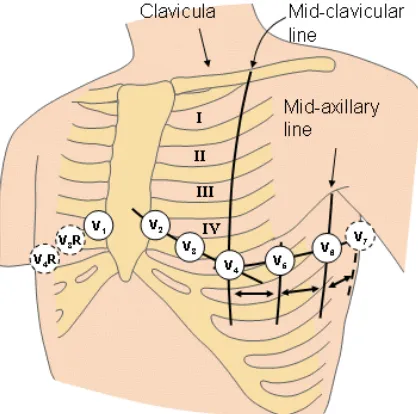
Figure 1-1. Illustration of precordial lead placement on a human subject. ... 15

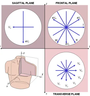
Figure 1-2. Graphical representation of the lead vectors captured with a 12-lead ECG. This model assumes a spherical conductor (white circle) and a centrally located single dipole source for the cardiac signals. ... 17

Figure 2-1. Plot of original and reconstructed leads for a male, age 35, of the healthy control group. Leads were reconstructed from Dawson’s transformation on a set of Frank XYZ leads. .. 31

Figure 2-2. Plot of original and reconstructed leads for a male, age 55, of the healthy control group. Leads were reconstructed from Dawson’s transformation on a set of Frank XYZ leads. .. 32

Figure 2-3. Plot of original and reconstructed leads for a male, age 46, of the myocarditis test group. Leads were reconstructed from Dawson’s transformation on a set of Frank XYZ leads. .. 33

Figure 2-4. Plot of original and reconstructed leads for a female, age 64, of the cardiomyopathy test group. Leads were reconstructed from Dawson’s transformation on a set of Frank XYZ leads. ... 34

Figure 2-5 Plot of original and reconstructed leads for a male, age 41, of the myocarditis test group. Leads were reconstructed from Dawson’s transformation on a set of Frank XYZ leads. .. 35

Figure 2-6 A graphical display of the correlation between the independent components generated from precordial lead pairs. A high level of correlation between the pairs means that the ICs that were generated from one set could be used to generate the other set of precordial leads. ... 38

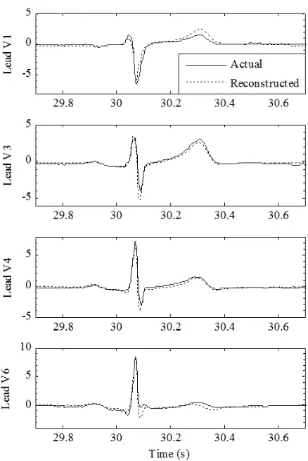
Figure 3-1 Comparisons of actual precordial leads and those reconstructed from the ICs of leads V2 and V5. This patient (s0055) had the closest correlation values across all precordial leads to the mean of the database at 30 seconds after the training period ... 44

Figure 3-2 Histograms of the reconstruction correlation percentages for each of the reconstructed leads. ... 47

Figure 4-1. Flow diagram of proposed method for 12-lead ECG reconstruction from a reduced lead set using ICA ... 53

Page 8 of 93

Figure 4-3. Typical example of reconstructing 12-lead ECG with the proposed method using reduced lead set of X, Y and Z. The blue curves are the original leads of patient S0001 and the red curves are the reconstructed versions. The average percent correlation across all leads is 96.73%. ... 60

LIST OF TABLES

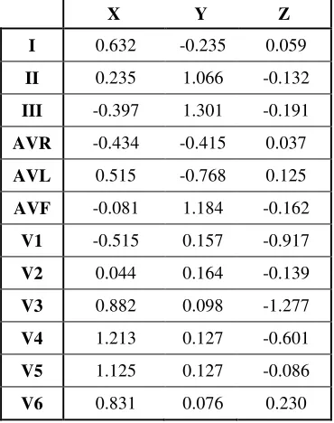
Table 2-1. Coefficients of the Dower Transform for the mixing matrix that computes the standard 12-leads from a VCG lead base. ……… 28

Table 3-1. Statistics of correlations between actual and reconstructed leads for precordial lead reconstruction using the reduced lead set: leads V2 and V5 ………. 46

Table 4-1. Statistics of correlations between actual and reconstructed leads for reconstruction using the reduced lead set: leads I, II, and V2 ………... 58

Table 4-2. Statistics of correlations between actual and reconstructed leads for reconstruction using the reduced lead set: Frank’s XYZ leads……….. 59

Page 10 of 93

SUMMARY OF CONTRIBUTIONS

This research effort focused on reconstructing electrocardiogram (ECG) leads from

reduced lead sets using independent component analysis (ICA) and culminated in the generation

and testing of two algorithms, each of which generated a publication.

1. Precordial lead ECG Reconstruction

An algorithm to reconstruct precordial leads from a two lead set was

developed. Leads V2 and V5 were found to be optimal and generated results with the

highest correlation between original and reconstructed leads.

Ostertag MH and Tsouri GR. Reconstructing ECG Precordial Leads from a Reduced Lead Set Using Independent Component Analysis. 33rd International Conf. of the IEEE Engineering in Medicine and Biology Society (EMBC ’11): 4414-4417, Aug. 30 2011-Sept. 3 2011.

2. Clinical, 12-lead ECG Reconstruction

The precordial lead ECG reconstruction algorithm was expanded and

improved to reconstruct the entire clinical, 12-lead ECG from a three lead set. Leads

I, II, and V2 were found to produce the best results of the standard lead arrangement.

Frank XYZ leads were also used. This algorithm was compared to state-of-the-art

reconstruction algorithms and compared.

Tsouri GR and Ostertag MH. Patient-Specific 12-lead ECG Reconstruction from Sparse Electrodes using Independent Component Analysis. IEEE Journal of Biomedical and Health Informatics, PP(99): 1, December 2013.

1.

INTRODUCTION

For patients released after cardiac surgery, those who have an arrhythmia that only

presents in certain circumstances, athletes seeking ideal training conditions, and medics

overseeing warfighters in the heat of battle all want one capability: remote physiological

monitoring. Remotely monitoring an individual’s electrocardiogram (ECG) can provide critical

information about the health of the subject. Currently, the products for measuring and recording a

patient’s ECG fail to provide a full set of clinically relevant data.

Remote, wireless ECG monitoring is close at hand, though, with only a few technical

hurdles left to overcome. One of these hurdles involves seamlessly incorporating these sensors

into patients’ lives in a non-invasive and foolproof manner. The devices are rapidly becoming

smaller and smaller, making them unobtrusive to the casual observer, and the next step is to

reduce the number of sensors required while keeping the system robust. Even though the number

of sensors that are monitoring the heart is reduced, medical professionals still need to see all

12-leads of the electrocardiogram to make diagnoses. The information is fundamentally missing

without the sensors present to record it, but it can be reconstructed from the other leads with

varying degrees of success.

The three prominent types of lead reconstruction transforms are the universal,

population-specific, and patient-specific transforms. Based on many works in the past, it is widely accepted

that universal transforms, which are developed and intended to work for all people, are not

reliable due to the wide degree of variance across patients and across time. Each patient has a

different composition of chest tissues, different size, shape or location of the heart, and different

levels of aging and disease. Population-specific transforms have proven to be more effective than

Page 12 of 93

classification, the transform becomes much more customized and produces a more accurate

reconstruction of missing leads for that set of patients. The most accurate transform is

patient-specific. Even in carefully selected groups, there still exist anatomical and diagnostic differences

between each person. By generating a transform that is specific to an individual, the best possible

reconstruction occurs. In all cases, the transforms are constant and do not adapt to changes over

time. As with all biological systems, change is a constant; shifting positions, changing activity

levels, and even breathing can affect how well any of the transforms can accurately reproduce the

missing information. Reducing the number of sensors is only half the problem, though. The other

half is maintaining the robustness of the system, which depends on solving a current problem

with ECGs: electrode misplacement.

Electrode misplacement is a common problem in electrocardiography caused typically by

human error. Although an electrode may only be misplaced by a small distance, that misplaced

electrode can change the morphology of a patient’s ECG waveform, leading to a misdiagnosis.

Reducing the effect of this error will not only help hospitals in the accuracy of short- and

long-term monitoring of patients but also increase the convenience of caregivers that place the

electrodes. The goal of this research was to use independent component analysis (ICA) to reduce

this misplacement error and reduce the number of electrodes needed for a clinical 12-lead ECG

measurement.

1.1

I

E

Electrocardiography provides clinicians with a non-invasive tool that provides detailed

insight into the working of a patient’s heart. Each time the muscles of the heart contract, they

pattern of coordinating contractions, which efficiently move blood throughout the pulmonary and

circulatory systems of the body. Due to the conduction of human tissue, these patterns of

depolarization that originate within the cardiac muscles create small, yet measureable signals on

the surface of the skin that (after being filtered and amplified) provide useful diagnostic

information about the condition of the heart.3

The first prototype system was developed in 1887 by Augustus Désiré Waller, who

placed each limb in a saline solution and used a capillary electrometer to observe the electrical

signals of his own heart.4 It has come a long way since its inception in the late 19th century, both

the technology and the diagnostic capabilities. Today, most cardiologists use a 12-lead system,

which consists of measurements from ten different electrodes. Electrodes placed on the right arm,

left arm, and left leg make up a set of limb leads and a fourth electrode is placed as a reference on

the right leg to either passively or actively reduce noise. The precise placement of the limb leads

is not critical since the limbs are far enough away from the heart that the region is roughly

isopotential. The limb leads provide information of the heart in the frontal plane, which bisects

the body from front to back, and are calculated from the limb electrodes as follows:5

= − (1.1)

= − (1.2)

= − (1.3)

where VI , VII , and VIII represent the three limb leads and φRA , φLA , and φLL represent the potential

at the right arm (RA), left arm (LA), and left leg (LL), respectively. From these leads, a set of

augmented leads was also developed. The augmented leads contain redundant information but

Page 14 of 93

between the one limb electrode and the Wilson’s central terminal, which is the average of the

three limb leads and serves as a reference. While the limb leads provide a look at the activity of

the heart, they are limited to the frontal plane of the body and are typically positioned too distant

from the source to pick up smaller, localized signal irregularities. The addition of precordial leads

solves both of these problems.

The precordial leads consist of a set of six leads placed on the upper thorax as shown in

Figure 1-1. They are spatially close to the front face of the heart and wrap around the chest from

the fourth intercostal space on the right of the sternum to the fifth intercostal space on the left

midline of the torso.4 Due to this spatial proximity, the precordial leads can be used to isolate

signal irregularities that may be difficult to diagnose using the limb leads. The precordial lead

measurements represent the vector from the Wilson’s central terminal to the precordial electrodes

and provide a view of the conduction pathways of the heart in the transverse plane. Without this

information, the dipole movement of the heart cannot be determined in three-dimensional space

and the diagnostic capability of the system is hindered. The six precordial leads (V1 through V6),

the three limb leads, and the three augmented leads form the 12-lead electrograph system, which

aids in diagnosing diseases from atrial hypertrophy to bundle-branch blocks to ventricular

fibrillation.3

Although the electrocardiogram has 12 leads, much of the information is redundant. This

should be readily apparent within the limb leads, which are all based on the difference between

three electrodes, but it also holds for the augmented leads, which are derived from the average of

the limb leads and are based upon the same measurements from the three limb electrodes. The

reason for the redundancy is the ease of recognizing patterns for cardiologists, who can more

easily make a diagnosis by comparing two similar leads at slightly varying angles. This diagnosis

Figure 1-1. Illustration of precordial lead placement on a human subject.5

Using body surface potential distributions as measured on the surface of the skin, the goal

of the inverse problem is to determine the underlying electrical activity of the heart. The actual

source of electrical activity cannot be uniquely determined when the cardiac region is

inaccessible because many different equivalent sources can generate the same set of surface

potentials.6 With the help of modern medicine’s understanding of the anatomy and physiology of

the human heart, the problem can be greatly simplified, and the source of the electrical signals

can be approximated with a high degree of accuracy. This allows for an initial clinical diagnosis

to be made, which typically needs to be verified by other methods, such as auscultation,

angiography, or imaging.4 Geselowitz found that modeling the source of cardiac electrical activity

as a single dipole could account for more than 90% of the activity seen within the heart.7 Using

this approximation, two limb leads and a single precordial lead (V2) contain the vast majority of

information about the contraction pattern of the heart. The information contained in the three

leads can be used to reconstruct the full 12 leads through a series of weighted sum transforms.

Page 16 of 93

set of coefficients, which are optimized on a per-patient basis or for a larger population. These

reconstructions have had varying degrees of success, depending on whether the transform was

tailored to the individual or a universal solution.8,9,10,11The success of the reconstruction of

missing leads from a reduced lead set is heavily dependent on the similarity of the ECG

waveform from beat to beat for individual-specific transforms or similarity between patients for

universal or group-specific transforms.

While the variability between patients, termed inter-individual variability, is to be

expected due to varying body compositions and heart location and orientation, the variability

from measurement to measurement of a single patient, termed intra-individual variability, is a

cause for concern for lead reconstruction because of the potential of a misdiagnosis. All current

lead reconstruction techniques rely on the stability of the initial conditions, which were present

during the training of the algorithm. Since the algorithm depends on the coefficients that were

developed during this training period, the reconstruction algorithms can only accurately

reconstruct the missing ECG leads if the relationship between all of the leads remains similar to

the original period. An act as simple as sitting up can change the position of the heart, thereby

fundamentally changing where the electrical sources of contraction are in relation to the

electrodes, which serve as observation points. The intra-individual ECG variability can be

classified into two major categories: beat-to-beat variability and session-to-session variability.

The former is due to changes in respiration rate, heart rate, posture, or noise and the latter is due

mainly to electrode misplacement. A misplaced electrode observes the electrical activity of the

heart from a different angle than an ideally placed electrode. This difference in observation can

result in a change in waveform morphology and potentially a misdiagnosis. In several accuracy

studies, nurses were found to place the electrodes accurately during only 13% to 25% of the

the redundancy of information by reducing the number of leads; by the same token, this makes

them highly susceptible if one lead was misplaced. The error of a misplaced base lead would be

present in each lead that it reconstructed. Both the inter-individual and intra-individual variability

issues may be able to be solved with a statistical method known as independent component

analysis.

Page 18 of 93

1.2

I

C

A

Biomedical signals are typically recorded with a known spatial distribution of multiple

sensors, and the resulting multichannel recording contains temporally and spatially correlated

measurements. The signals of interest are rarely recorded in isolation because as the signals travel

through the body, they become mixed with background activity and noise, which make the

sources within the body challenging to analyze. By applying independent component analysis

(ICA) to these mixed signals, the underlying, independent sources can be uncovered.13

ICA separates out mixed signals into their independent components by exploiting their

independence. This independence is found by focusing on finding sources that are the most

non-Gaussian. When combined, the joint density of Gaussian sources is completely symmetric,

making it impossible to estimate the individual independent sources.14 If there is only one

component with Gaussian distribution, it can be separated from the others, which has been

utilized in ECG noise removal.15 Any number of mixed non-Gaussian sources results in an

asymmetric distribution, which can then be separated as long as there are at least as many

observation points as sources. Each observation consists of a linear combination of the

independent sources; the coefficients of this linear combination form a mixing matrix.

This mixing matrix provides insight into the relative projection strengths of the respective

independent components onto each of the sensors, and by multiplying the underlying independent

sources by the mixing matrix, the original observations can be reproduced. By multiplying the

sensor data by the unmixing matrix that is also obtained at the end of ICA training, a new matrix

will be generated that consists of rows of statistically independent components. The basic linear

models relating the sensor data, independent components, mixing matrix, and unmixing matrix

= and = (1.4)

where the vector represents ‘m’ independent sources, the vector represents an approximation

of , the matrix represents the linear mixing of the sources, the matrix is the linear unmixing

matrix, and the vector is composed of ‘m’ observed signals.13 The mixing matrix is square in

most popular ICA algorithms in order to exploit the inverse matrix to shorten the time of

convergence.

The goal of ICA is to generate the mixing matrix that relates the independent components

to a set of observations; many different methods have been developed to reach this goal. The

research in this paper was done with the FastICA algorithm developed by Hyvärinen and Oja.14

This method seeks to maximize the non-Gaussianity of the resultant independent components by

recursively maximizing both the kurtosis and negentropy of the signals. Kurtosis is the

forth-order cumulant of a signal and is zero for a random Gaussian source. The kurtosis of a signal is

defined as seen in Eq. 1.5.

= !_{" − 3} $_"$ _(1.5)

Before calculating the kurtosis of a signal in the FastICA, the signal is preprocessed to have unit

variance, and the algorithm can be simplified to Eq. 6:

= !_{" − 3 (1.6)}

Negentropy has been shown with statistical theory to be a good measure of non-Gaussianity, and

Page 20 of 93

given variance. While it is very useful for determining non-Gaussian sources, it is difficult to

measure without knowledge of the probability distribution function. In the FastICA algorithm, the

negentropy is approximated using formulae developed by Hyvärinen.

% = [ ' − '"($ _(1.7)

') =_*)₊log/0ℎ2) and '_$ = − exp 6−7_$89 (1.8)

where % is the negentropy approximation for any non-quadratic function ', '₎ and '_$ are

convergent functions used to approximate the negentropy, and 2₎ is a constant between 1 and 2.

These functions and their derivatives are simple to calculate and are central in converging to

consistent sets of independent sources.

The FastICA algorithm first works by removing the mean from all signals, a process

called centering, and then performing principal component analysis to create a set of orthogonal

signals from the observations. The mixing matrix resulting from these two operations is then run

through a recursive routine that maximizes both the kurtosis and negentropy of the original

sources, thus minimizing the Gaussianity and generating the underlying, independent sources.

The optimized mixing matrix provides a linear transform between the independent sources or

components and the observed signals as seen in Eq. 1.4.

In previous research, ICA has been successfully applied to the electrocardiogram, which

satisfies some of conditions of ICA: the different signal sources of cardiac contraction are linearly

mixed at the ECG electrodes, the time delay in signal propagation is negligible, and there are

generally fewer sources than sensors. The electrocardiogram does violate the ICA assumption of

spatial stationarity, though, since the heart moves during every contraction. This movement may

of ICA to the ECG is the separation of maternal and fetal heartbeats from electrodes placed on the

mother’s chest and abdomen. In the initial signal, the fetal heartbeat cannot be seen, but after

performing independent component analysis, there are clearly two heartbeats, one at 72 bpm and

the other at 106 bpm. By recombining the channels that reflect the mother’s heartbeat separately

from the channels of the fetus and by zeroing out the noisy source, the two heartbeats can be

separated and analyzed independently.16 Other examples include separating noise and artifacts

from the desired signals15 and differentiating mixed biopotentials from each other, such as

separating the interference of the muscle contractions from a blink from an electroencephalogram

(EEG) reading13.

Overall, the concept of applying ICA to ECG monitoring technology is very promising,

and if used properly, can result in reduced noise levels, which commonly plague many

biopotential measurements, and in isolating the independent signals of the heart, allowing for

separation and reconstruction of the cardiac signals. This technology relies heavily on the number

of sources being less than the number of observation points. The sources of the cardiac signal can

be approximated by a dipole model, but in reality, each individual’s heart and specific condition

may have a different number of sources.6 Another potential source of issue is the unordered

nature of the results. ICA may be able to produce independent sources for a set of observations,

but the order is dependent on the convergence of the system to the source that is the least

Gaussian. The unordered independent sources can cause issue for algorithms relying on

consistent convergence to the same components. By imposing spatial and temporal restraints on

the ICA algorithms, more ordered and detailed analysis may be performed and these issues can be

Page 22 of 93

2.

INITIAL RESEARCH

In initial testing, it was quickly shown that static, universal transforms from a reduced set

of stationary leads to the full 12-lead ECG were not effective at reproducing cardiac signals

(Section 2.3). The universal transform relies on the flawed model that all patients are similar.

Patient- and population-specific transforms showed a much better rate of success.11 In addition to

simply reconstructing missing leads, a patient-specific transform utilizing independent component

analysis (ICA) showed promise for developing a method to reduce the error caused by electrode

misplacement, both in clinical and residential settings, by accurately reproducing the same

underlying sources of ECGs from different sets of leads. By using different sets of leads, the

initial experimentation with generating independent sources from standard precordial leads

represented an extreme case of misplaced sets of electrodes (Section 2.4). The following initial

inquiry into using ICA lead to the development of the reconstruction algorithms in Section 3 and

2.1

S

A

For the reconstruction of missing leads in a reduced lead system, the use of a universal

matrix is not appropriate. The recent work by Dawson10 only marginally improves on the

universal transforms that Dower developed over 40 years ago,9 and the new transformation matrix

that was developed through regression of a linear affine transformation still suffers the problem of

changing the morphology of the waveform. The research done by de Charzal and Celler support

the previous statement that the use of a universal matrix is inappropriate.17 They found that some

applications of the universal transform worked perfectly (correlation of 1.00) but others resulted

in negative correlations as large as -0.63. The future of transformation matrices lies in matching

them to patients through individual adjustments as performed by Man et al.18 or by placing

patients in predefined populations that have population-specific coefficients.11

The traditional 12-lead ECG system produces a substantial amount of redundant

information, which helps at offsetting the effect of electrode misplacement. If one electrode is

misplaced, which happens quite regularly according to Schijvenaars and references,12 the

cardiologists can still make a diagnosis because the information that was contained in that lead is

also present in others. On the other hand, the misplacement of an electrode in a 3-lead VCG

system can invalidate the entire set of measurements. The lack of redundancy and reliability is a

problem in the current reduced lead systems. They are problems that independent component

analysis (ICA) may be able to help solve. ICA can determine the underlying independent sources

of a biosignal, regardless of the placement of the electrodes. In a simple model, the electrical

activity of the heart is a single dipole, which is comprised of three statistically independent,

orthogonal sources. Gulrajani elaborates on the different models that could be used,6 but the

single dipole model is the simplest and only requires a minimum of three leads to unmix to the

Page 24 of 93

noise source could be found with ICA, and with simple statistical algorithms, the noise could be

automatically eliminated for a cleaner, more recognizable signal.15

ICA has not yet been used to compensate for electrode misplacement but this could well

be the future of ECG monitoring. By performing constrained ICA, only one or two electrodes

need to be carefully positioned. These electrodes would be used as references, generating two of

the three sources from a single dipole model, and all subsequent sources could be generated by

haphazardly placed electrodes. Since the position of the initial electrodes is known and assuming

that the patient has a set of patient-specific or population-based transform coefficients, the

traditional 12-lead electrocardiogram can be reproduced in its entirety from a minimal number of

leads without fear of misdiagnosis from the main source of intra-individual variability, electrode

misplacement. This “opportunistic” ECG system is a promising technology of the future, but in

order for it to work, the independent components must be able to be reliably generated with a

2.2

S

F

M

In order to properly compare the results during algorithm development, the first step in

the process was to establish a measure of similarity by which the derived ECG leads can be

compared to the originals. Several different methods already existed and were regularly used for

determining a quantitative measure of error between two signals.

The root-mean-square (RMS) error calculation has been applied across a broad range of

data types and serves as a well-known method of comparison. It was not the most promising

option for comparing sets of independent components or two electrocardiogram (ECG) signals,

though. For one, only portions of the entire signal are utilized by cardiologists for diagnosis. A

small offset error in an irrelevant section of the signal, such as the flat portion between beats,

could contribute a large portion to the RMS error while not affecting the clinical relevance of the

signal. Due to this, a signal with poor performance in the flat region but perfect performance in

the PQRST region could have the same RMS error as a signal with a perfect flat region and a

PQRST region with a changed morphology. The option does exist to selectively perform RMS

calculations, either by using it over specific regions or weighting different regions more heavily

than others.

The next option for a measure of similarity was calculating the cross-correlation between

the signals under question. Correlation was used by de Charzal and Celler for analyzing the

validity of universal linear transformation matrices17 and it could easily be applied to the case of

independent components, which are also linear transforms of the original leads. Cross-correlation

had the benefit of not being affected by a constant offset between the signals and produced

reasonable results when the signals under comparison were negatives of one another as occurs

Page 26 of 93

negative of itself is -1 but the RMS error between the two signals would be unable to represent

the visibly apparent similarity of the signals.

These measures of similarity were compared with others, such as the Kullbeck-Liebler

distance, subjective fidelity comparison, or the peak signal-to-noise ratio, but they were not found

to accurately and quantitatively capture the desired results. Since the best option should perform a

qualitative comparison of the clinical relevance of a modified signal to the original, a metric of

cross correlation percentage was selected. The selected measure was used to compare sets of

independent components that were derived from various lead sets, which consist of two leads for

reconstructing the precordial leads and three leads for reconstructing the full 12-lead set that exist

in a three-dimensional space. The reduced lead sets were drawn from the 12 traditional leads and

the Frank XYZ leads, which were found in various databases such as the Physikalisch-Technische

Bundesanstalt ECG database. The specific figure of merit and its application can be seen in

2.3

V

U

T

M

V

Much work has been done in recent years to find a universal matrix that could synthesize

a standard 12-lead electrocardiogram from a reduced set of leads. One of the pioneers of creating

reduced lead systems was Dr. Earnest Frank. He researched and mapped body surface potentials

and used this work to create a set of orthogonal leads (X, Y, and Z), which became one of the top

contenders in reduced lead systems, along with the EASI system.8 The Frank leads led to a new

type of electrocardiographic monitoring called vectorcardiography. Ever since Frank popularized

this set of leads, researchers have been attempting to find a universal transform from the

three-lead system to the traditional 12-three-lead, which is most familiar to cardiologists. The pioneering

research was performed by Dower, and the resulting “universal” transform was termed the Dower

transformation matrix.9 In 2009, Dawson and colleagues refined the transformation matrix to

obtain a slightly lower root-mean-square error than the traditional Dower transformation.10They

accomplished this by using an affine linear model as opposed to the strictly linear model used by

Dower. The affine linear model includes a constant that is unrelated to the reduced lead set, and

its inclusion in the model allows the model to compensate for errors introduced by an incorrect

source model or drift biases.

Developing the Transform Matrix

The algorithm for developing Dawson’s affine linear transform proceeds as follows: first,

the Physikalisch-Technische Bundesanstalt Database (PTBDB) patients were divided into healthy

control (HC) and myocardial infarction (MI) patients. The PTBDB contains the standard 12-lead

Page 28 of 93

of each recording were extracted and least-squares fitting was performed on the transform model

seen in Equation 2.1:

: = ; + = = 2> + 2)) + 2$$ + 2?? + = (2.1)

where the vector X contains the three orthogonal leads, the matrix A is the XYX to 12-lead

transformation matrix, and the vector Y contains the calculated 12-lead ECG. In order to obtain

statistically consistent coefficients, at least 25 different patient recordings were needed for both

the HC and MI groups. These coefficients were used to calculate a 12-lead ECG, which was

directly compared with the recorded 12-lead from the database using the R2 metric. The R2 values

resulting from applying Dawson’s transforms were compared to those resulting from applying

Dower’s universal matrix with higher R2 values relating to a closer relationship between the

transformed and original leads. A different method was used for generating the inverse

transforms. Due to the redundancy of the information contained in an 8-lead system, principal

component analysis (PCA) was performed to reduce the redundant information and find a

consistent transformation. The set of coefficients that Dawson et al. obtained by following the

Table 2-1

Coefficients of the Dower Transform for the mixing matrix that computes the standard 12-leads from a VCG lead base.

X Y Z

I 0.632 -0.235 0.059

II 0.235 1.066 -0.132

III -0.397 1.301 -0.191

AVR -0.434 -0.415 0.037

AVL 0.515 -0.768 0.125

AVF -0.081 1.184 -0.162

V1 -0.515 0.157 -0.917

V2 0.044 0.164 -0.139

V3 0.882 0.098 -1.277

V4 1.213 0.127 -0.601

V5 1.125 0.127 -0.086

V6 0.831 0.076 0.230

Performing Morphological Comparisons

The same 15-lead database that was used for developing the transform coefficients was

used to test their validity. Using Matlab 2009, two-second clips of patients ECG recordings were

taken for lead I, lead II, and lead V4. These leads were selected because they offer unique

morphologies and have low (78.30), high (92.27), and medium (89.06) R2 values in comparison

to their transform group.6 For several patients, these three leads were calculated from the Frank

XYZ leads provided using the coefficients in Table 2-1. The original and newly constructed

signals were normalized to have a range of 1 and the mean of each signal was removed. The two

signals were then plotted on the same plot with the original ECG signal in solid blue and the

Page 30 of 93 Results

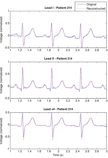
Five of the patients tested were part of the healthy control group and a representative

sample can be seen in Figure 2-1. and Figure 2-2.. For these patients, the reconstructed lead most

closely matches the original signal for lead II and closely matches for lead V4 with the exception

in the amplitude of the ST region. For the same set of patients, lead I shows significant

morphological changes in the P, Q and S waves between patients.

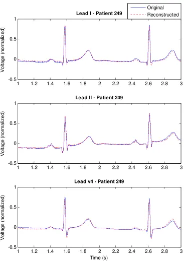
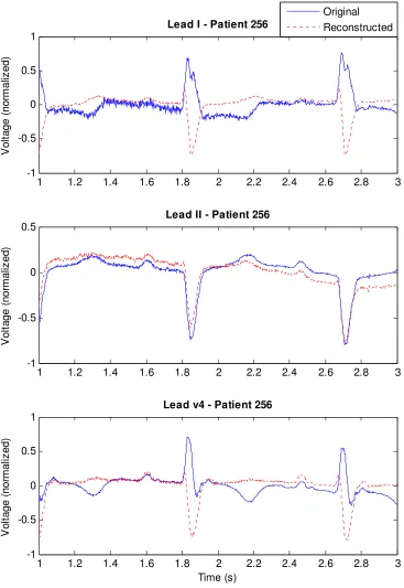
The next three patients in Figure 2-3. through Figure 2-5 have heart conditions but have

never had a myocardial infarction (MI). Patient 249 has myocarditis but the transform still

produces very accurate reconstructed leads with no significant morphological changes. The next

two patients have cardiomyopathy and myocarditis and the reconstructed leads I and V4 do not

Figure 2-1. Plot of original and reconstructed leads for a male, age 35, of the healthy control group. Leads were reconstructed from Dawson’s transformation on a set of Frank XYZ leads.

1 1.2 1.4 1.6 1.8 2 2.2 2.4 2.6 2.8 3

-0.5 0 0.5 1

Lead I - Patient 214

V o lt a g e ( n o rm a liz e d ) Original Reconstructed

1 1.2 1.4 1.6 1.8 2 2.2 2.4 2.6 2.8 3

-0.5 0 0.5 1

Lead II - Patient 214

V o lt a g e ( n o rm a liz e d )

1 1.2 1.4 1.6 1.8 2 2.2 2.4 2.6 2.8 3

-1 -0.5 0 0.5

Lead v4 - Patient 214

Page 32 of 93

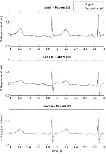
Figure 2-2. Plot of original and reconstructed leads for a male, age 55, of the healthy control group. Leads were reconstructed from Dawson’s transformation on a set of Frank XYZ leads.

1 1.2 1.4 1.6 1.8 2 2.2 2.4 2.6 2.8 3

-0.5 0 0.5 1

Lead I - Patient 229

V o lt a g e ( n o rm a liz e d ) Original Reconstructed

1 1.2 1.4 1.6 1.8 2 2.2 2.4 2.6 2.8 3

-0.5 0 0.5 1

Lead II - Patient 229

V o lt a g e ( n o rm a liz e d )

1 1.2 1.4 1.6 1.8 2 2.2 2.4 2.6 2.8 3

-0.5 0 0.5 1

Lead v4 - Patient 229

Figure 2-3. Plot of original and reconstructed leads for a male, age 46, of the myocarditis test group. Leads were reconstructed from Dawson’s transformation on a set of Frank XYZ leads.

1 1.2 1.4 1.6 1.8 2 2.2 2.4 2.6 2.8 3

-0.5 0 0.5 1

Lead I - Patient 249

V o lt a g e ( n o rm a liz e d ) Original Reconstructed

1 1.2 1.4 1.6 1.8 2 2.2 2.4 2.6 2.8 3

-0.5 0 0.5 1

Lead II - Patient 249

V o lt a g e ( n o rm a liz e d )

1 1.2 1.4 1.6 1.8 2 2.2 2.4 2.6 2.8 3

-0.5 0 0.5 1

Lead v4 - Patient 249

Page 34 of 93

Figure 2-4. Plot of original and reconstructed leads for a female, age 64, of the cardiomyopathy test group. Leads were reconstructed from Dawson’s transformation on a set of Frank XYZ leads.

1 1.2 1.4 1.6 1.8 2 2.2 2.4 2.6 2.8 3

-1 -0.5 0 0.5 1

Lead I - Patient 256

V o lt a g e ( n o rm a liz e d ) Original Reconstructed

1 1.2 1.4 1.6 1.8 2 2.2 2.4 2.6 2.8 3

-1 -0.5 0 0.5

Lead II - Patient 256

V o lt a g e ( n o rm a liz e d )

1 1.2 1.4 1.6 1.8 2 2.2 2.4 2.6 2.8 3

-1 -0.5 0 0.5 1

Lead v4 - Patient 256

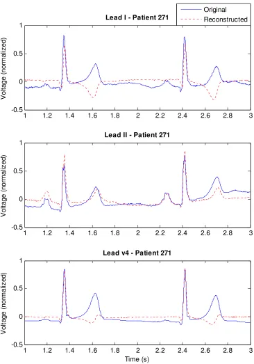
Figure 2-5 Plot of original and reconstructed leads for a male, age 41, of the myocarditis test group. Leads were reconstructed from Dawson’s transformation on a set of Frank XYZ leads.

1 1.2 1.4 1.6 1.8 2 2.2 2.4 2.6 2.8 3

-0.5 0 0.5 1

Lead I - Patient 271

V o lt a g e ( n o rm a liz e d ) Original Reconstructed

1 1.2 1.4 1.6 1.8 2 2.2 2.4 2.6 2.8 3

-0.5 0 0.5 1

Lead II - Patient 271

V o lt a g e ( n o rm a liz e d )

1 1.2 1.4 1.6 1.8 2 2.2 2.4 2.6 2.8 3

-0.5 0 0.5 1

Lead v4 - Patient 271

Page 36 of 93 Discussion

While the Dawson’s coefficients may have an average R2 value of 84.79 for the health

control patients, the so-called universal matrix does not accurately reproduce the morphology of

the original ECG waveform for all leads. The results seen below also question the appropriateness

of population-based coefficients. The patients in Figure 2-1. to Figure 2-3. and Figure 2-5 are all

males between the ages of 35 and 55. The first two are healthy controls and the last two have

been diagnosed with myocarditis. These patients are very similar and would likely belong to the

same group classification, but the transform matrix does not perform equally well across them.

The patients in Figure 2-1. and Figure 2-2. demonstrate a reconstructed ECG that is almost

perfectly correlated to the original while the patient in Figure 2-3. through Figure 2-5 shows a

reconstructed ECG that has very poor correlation. This range in correlation using universal

transformations matches the results seen in a previous study by de Charzal and Celler.17

The R2 value for the reconstructed leads is deceptively high for the level of

morphological error seen when performing the lead transforms. Although the RR, QT, and ST

intervals have remained relatively constant through the transform, the claim that the linear affine

transformation matrix should be used for diagnoses requiring use of the waveform morphologies

is strongly questioned. Significant variability in the level and type of introduced error has been

observed and the use of a universal matrix for VCG to 12-lead ECG transforms may be

inappropriate. Patient-specific coefficients have been shown to produce much better results11,17

2.4

V

S

I

C

A

ECG

L

Before ICA could be applied to reduce the error caused by electrode misplacement, the

spatial stationarity of the independent components (ICs) was validated across the set of standard

12-leads. ICs were generated from varying pairs of leads from the standard 12-lead set using the

FastICA algorithm.14 The ICs were manually ordered such that each set of ICs was matched with

similar looking ICs from the lead sets under consideration. A correlation calculation was

performed between each similar IC pair and the lowest correlation value among all generated ICs

was recorded and displayed in the colorplot in Figure 2-6.

During this process, it was found that the ICs that were generated with any two

combination of leads I, II, III, AVR, AVL, and AVF and a precordial lead had very high

similarities to the ICs generated by any other combination of the aforementioned leads and the

same precordial leads. This finding is supported by the method in which the ECG data is

obtained. Leads I, II, and III are measured using shared points on the torso, which allows any lead

to be calculated from the other two; AVR, AVL, and AVF are augmented leads that are also

calculated based on the limb leads. Since any two leads contain all of the relevant information

about all six, it follows that their independent components should be the same, which was found

to be true.

After the first confirmation of the potential power of ICA, the correlation between ICs of

different precordial lead pairs was examined to determine if a similar sort of spatial independence

existed. The same level of correlation between different lead sets for the limb leads was not seen

in the precordial leads, but there was a relatively high level of correlation between the ICs

generated from proximal lead sets. For example, precordial leads V3/V5 generated similar ICs to

Page 38 of 93

an extreme case of electrode misplacement. The success at generating similar ICs was very

promising and lead to the development of the first algorithm, which reconstructed missing

precordial leads (Section 3).

Figure 2-6 A graphical display of the correlation between the independent components generated from precordial lead pairs. A high level of correlation between the pairs means that the ICs that were generated from one set could be used to generate the other set of precordial leads.

ICs from Precordial Le ad Sets

IC s fr o m P r e c o r d ia l L e a d S e ts

Correlation of Independent Components between Precordial Lead Pairs

3.

RECONSTRUCTING ECG PRECORDIAL

LEADS USING INDEPENDENT COMPONENT

ANALYSIS

In this section, precordial lead reconstruction from a reduced set of leads is considered.

We propose the use of independent component analysis to train patient-specific transforms from a

reduced lead set to the six precordial leads of the standard 12-lead electrocardiogram. The

proposed approach is applied to a publicly available database comprising 549 ECG recordings of

patients with varying cardiovascular conditions. The fidelity of reconstruction is measured using

percent correlation between the actual and reconstructed signals following a 30 seconds time

lapse. The mean correlation is over 95% with a standard deviation under 12.7% for all

reconstructed leads. The results demonstrate the potential of the suggested approach to provide a

reliable solution to precordial leads reconstruction. This research was presented at the 33rd

International Conference of the IEEE Engineering in Medicine and Biology Society in 2011.1

3.1

I

The electrocardiogram (ECG) is the most common procedure for diagnosing

cardiovascular problems and a critical tool for long-term monitoring of patients.19 While most

physicians prefer the diagnostic capabilities of traditional 12-lead systems, it is commonly not

fully implemented for patient comfort and caregiver convenience.

Of the 10 electrodes used in a 12-lead system, the most problematic are the unipolar leads

across the precordium, of which leads V3 and V4 can complicate diagnostic procedures, such as

Page 40 of 93

precordial leads have substantial redundant information due to proximity and since their sources

can be approximated by a dipole, they are prime candidates for reduction by ICA.

In this section, we propose and investigate reconstructing precordial leads in a

patient-specific approach from their underlying sources using ICA. We are unaware of previous attempts

to use ICA for ECG lead reconstruction.

The rest of the section consists of an overview of the Proposed Method in Section 3.2, a

summary of the Results in Section 3.3 when applying the approach to a well-known and publicly

available ECG database, a Discussion in Section 3.4, and the Conclusion in Section 3.5.

3.2

P

M

The proposed precordial lead reconstruction follows a multi-stage approach. First,

preprocessing is performed on the ECG signal to condition it and to locate the QRS complexes.

Next, a training sequence is performed to obtain a set of patient-specific transforms () from the

independent sources of the precordial leads () to the full set () as seen in (3.1). Then, the excess

electrodes may be removed and the algorithm will continue to reconstruct the missing leads. In

what follows, each step is described in more detail.

= (3.1)

ECG Dataset and Preprocessing

The work presented in this paper used the Physikalisch-Technische Bundesanstalt (PTB)

diagnostic ECG database as made available through PhysioNet.21 The database contains 549 ECG

myocardial infarctions, and the remainder with other cardiac diagnoses. For each recording, the

12 traditional and three Frank leads were captured simultaneously at a sampling frequency of

1 kHz.

The preprocessing stage encompasses two steps: filtering and beat detection. A set of

cascading digital filters were used. The first was a high-pass filter with a cutoff frequency (@_A) of

0.5 Hz to remove the baseline drift. The second was a low-pass filter with an @_Aof 150 Hz to

reduce the amount of noise in the signal. Both filters were developed to meet AHA standards

(outlined in [19]) using the Parks-McClellan algorithm.22 The filtered signal was then put through

a QRS detection algorithm similar to the Pan-Tompkins QRS detection algorithm. A moving

average of 100 samples (100 ms) was taken of the square of the approximate derivative as

obtained with the function seen below:

[B( = −[B − 10( − 2[B − 5( + 2[B + 5( + [B + 10( (3.2)

The resulting function was normalized and the peaks were found that had a value above

the threshold of 0.125 and that occurred at least 200 ms from the previous peak. This length of

time was selected because it is the minimum time between beats due to physiological limitations.

Once the peaks were found, the beat domain was defined as spanning three-eighths the time

between the current and previous peak and five-eighths the time between the current and next

peak.

Transform Training Sequence

Leads V2 and V5 were used to reconstruct the other precordial leads due to their

Page 42 of 93

correlation between the ICs of various sets of precordial leads with those of V2 and V5. Using

ICA over the two leads generated two ICs, which represent the underlying sources as a dipole.

For training, we made use of all six precordial leads. The first valid beat was used as a

training sequence to determine a transform between the ICs of leads V2 and V5 and the missing

precordial leads V1, V3, V4, and V6. First, each lead had the mean removed and was normalized

to unit variance. Then, the 4-by-2 mixing matrix was generated to reconstruct the four missing

leads from the pair of ICs generated from leads V2 and V5. It was obtained by performing

FastICA14 on several sets of lead combinations that had previously shown to produce ICs that

were highly correlated to those of leads V2 and V5. As part of the ICA solving procedure, mixing

matrices are generated that relate the observations and ICs as seen in (3.1). The coefficients that

make up the mixing matrices of (V1,V5), (V3,V5), (V2,V4), and (V2,V6) were used to create a

new mixing matrix that could reconstruct V1, V3, V4, and V6, respectively. For example, the

application of ICA to leads V1 and V5 resulted in the square mixing matrix as seen in (3.3). The

elements relating to V1 were placed into a new 4-by-2 mixing matrix, which can reconstruct all

missing leads from a set of ICs (3.4).

GH)HIJ = K22H) LH)

HI LHIM KNO

)

NO$M

P

H)

H?

H!

HQ

R = S

2H) LH)

2H? LH?

2H! LH!

2HQ LHQ

T KNO_NO)

$M

Due to the non-ordered and sign-independent nature of ICA, the leads were sorted based

upon the correlations of each lead combination’s set of ICs with the (V2,V5) IC pair. The sorted (3.3)

reconstruction mixing matrix, the original ICs of V2 and V5, and the transform matrix between

the ICs and (V2,V5) were saved for future use.

Reconstruction Sequence

For reconstruction, we used leads V2 and V5 to reconstruct all other precordial leads.

Each beat after the training sequence was handled in the following manner. The mean of the beat

was removed and the variance normalized. Then, ICA was performed on V2 and V5, but instead

of using a random initial mixing matrix for the iterative solving procedure in the FastICA

algorithm, the original transform matrix was provided as an initial guess. This helped direct the

solution to a similar set of ICs and shortened the time of convergence.

Even though an initial guess was provided, the FastICA algorithm occasionally

converged to a switched or negative IC pair, which was sorted in the following manner. The

resulting IC pair and the original ICs that were generated during training were downsampled by a

factor of 5 and compared. A correlation function was formed that was the sum of the absolute

value of the correlations for the two possible configurations of ICs:

Config. 1 Config. 2

K|NO_|NO)0|

$0|M ≈ K

|NO)|

|NO$|M K

|NO)0|

|NO$0|M ≈ K

|NO$|

|NO)|M

Since the ICs were expected to match each other, configuration 1 was given a preferential

weight of 1.25. The two functions were compared by the above metric and the set that had a

higher maximum correlation was selected. The index of the maximum and individual correlation

Page 44 of 93

and the sorted reconstruction mixing matrix from the training sequence, V1, V3, V4, and V6 were

reconstructed from the ICs of (V2,V5) using (3.4).

Method of Comparison

In order to compare the actual lead signals to the reconstructed signals, a percent

correlation (W) was utilized as the figure of merit, which resembles the similarity coefficient used

in [25]. The percent correlation metric was calculated per lead in the following manner:

W = ∑\Z]+YZY[Z

^∑\_Z]+Y_Z8^∑\_Z]+Y[_Z8× 100% (3.6)

where the index value a represents the samples within a beat of length b samples, ;_c is the

original ECG signal, and ;[_c is the reconstructed ECG signal. A value of 100% represents perfect

correlation between the two signals while lower values indicate a worse timing alignment.

Correlation was used instead of other measures such as Root-Mean-Square Error (RMSE)

because correlation speaks to how well the timing of the signals is aligned rather than the absolute

value. In many applications of ECG, these timing features are much more critical than absolute

values.

The original and reconstructed waveforms were compared at several time instances after

the training sequence and the percent correlation values were plotted on a histogram. This

allowed for a direct, visual comparison of the changes in the fidelity of reconstruction over time.

3.3

R

We ran the precordial lead reconstruction algorithm over 548 of the 549 recordings in the

PTB database from the beat immediately following the training sequence (t=0 sec) to the beat that

Page 46 of 93

because the V1 lead was removed mid-recording. The histogram of the correlations can be seen in

Figure 3-2 and the statistically summary of the distributions can be found in Table 3-1.

Table 3-1

Statistics of correlations between actual and reconstructed leads for precordial lead reconstruction using the reduced lead set: leads V2 and V5

Time V1 V3 V4 V6

0 sec µ (σ) 91.7 (12.4) 97.5 (4.8) 95.8 (7.6) 96.8 (4.7) 30 sec µ (σ) 91.5 (12.6) 97.0 (7.4) 95.2 (8.9) 96.5 (5.0)

All leads were reconstructed with a high average correlation percentage and low

variance. Leads V3 and V6 had the best reconstructions on average (all above 96.4% for both 0

and 30 sec), followed by lead V4 (above 95.2% for both 0 and 30 sec). Lead V1 was

reconstructed with the lowest average correlation percentage (over 91.5% for both 0 and 30 sec)

and the largest standard deviation (under 12.7% for both 0 and 30 sec). This was expected as

problems in the atrium have a stronger effect on the signal recorded by lead V1 than the other

precordial leads due to V1’s proximity to that region of the heart.20 V1 was the most problematic

Figure 3-2 Histograms of the reconstruction correlation percentages for each of the reconstructed leads.

We found that the algorithm had difficulty accurately reconstructing irregular beats that

were not present in the training sequence. This was due to either a change in ICs or an error in the

sorting process and was most common in patients with dysrhythmia. When the irregular beats

were reconstructed, they looked differently than the typical heartbeat of the patient but did not

necessarily have the exact shape of the actual irregular beat.

Figure 3-1 presents an illustrative case of reconstruction of a patient 30 seconds after the

training sequence occurred. For presenting an unbiased sample, we chose to present a pulse with

reconstruction quality that most closely matches the mean correlation percentages, rather than the

50 60 70 80 90 100

0 0.05 0.1 0.15 0.2 0.25 0.3

Reconst. Lead V1

P er ce n t o f P at ie n ts

50 60 70 80 90 100

0 0.05 0.1 0.15 0.2 0.25 0.3

Reconst. Lead V3

50 60 70 80 90 100

0 0.05 0.1 0.15 0.2 0.25 0.3

Reconst. Lead V4

Correlation Percentage P er ce n t o f P at ie n ts

50 60 70 80 90 100

0 0.05 0.1 0.15 0.2 0.25 0.3

Reconst. Lead V6

Correlation Percentage t = 0 sec

Page 48 of 93

best reconstructed pulse. Due to the locations of V2 and V5, the interpolated leads, V3 and V4,

were reconstructed the best and the extrapolated leads, V1 and V6, had larger reconstruction

error. If the patient had been diagnosed with a problem in the atrium rather than an anterior

myocardial infarction, the reconstruction of lead V1 would have been much worse.

3.4

D

The algorithm was tested up to 30 seconds after the training period, but even in that short

amount of time, we were able to observe the adaptive nature of ICA. The reconstruction mixing

matrix from the ICs to the precordial leads remained constant but the transform from (V2,V5) to

their ICs changed with each beat. This feature results in a time-adapting and patient-specific

transform from (V2,V5) to the other precordials that can effectively adapt to changing beat

patterns. This is a clear advantage over static linear transformations.

Although the precordial reconstruction worked on the majority of patients with a high

level of fidelity, the system is susceptible to errors when patients have atrial conditions, which are

most strongly detected in lead V1.20 Since the reconstruction is based on the signals recorded at

V2 and V5, an issue that is present in lead V1 may not be accurately reconstructed. On the other

hand, an error in lead V2 or V5 will cause an error to be propagated across all reconstructed

leads. For patients who have displayed signs of dysrhyhmias or have atrial conditions, it is

suggested that lead V1 is not removed from the patient since it cannot be reliably reconstructed

and is important for accurate diagnosis. This can be checked in the initial training phase when all

six precordial leads are attached. The electrodes for lead V1, V3, V4, and V6 are removed after

Due to a lack in consistent methods and metrics in previously published works, our

reconstruction results are difficult to compare to other studies. Nelwan et al.23 performed

reconstruction of four missing precordial leads from V2 and V5 and found a median correlation

of 0.964 for a general set of coefficients and 0.994 for a patient-specific set. These numbers are

high for several reasons: first, they present the median correlation instead of the average, reducing

the effect of outliers that were present in our results; second, the ECG waveforms that were used

were the median complexes about a certain time; and third, all patients were of the same

diagnostic class and the most difficult to reconstruct, patients with arrhymias and left bundle

branch blocks, were excluded from the reconstruction test. In other work, the improved EASI

coefficients as derived by [26] were used to reconstruct the precordials with varying degrees of

success. The average correlations across the precordials with the improved coefficients range

from 0.919 to 0.941, which fall below our calculated average correlation of 0.950. Also, our

correlation calculations do not include leads V2 or V5, which would have perfect correlation

because they did not need to be r