parameter estimation
.
White Rose Research Online URL for this paper:
http://eprints.whiterose.ac.uk/3466/
Article:
Dewar, M. and Kadirkarnanathan, V. (2007) A canonical space-time state space model:
state and parameter estimation. IEEE Transactions on Signal Processing, 55 (10). pp.
4862-4870. ISSN 1053-587X
https://doi.org/10.1109/TSP.2007.896245
[email protected] https://eprints.whiterose.ac.uk/
Reuse
Unless indicated otherwise, fulltext items are protected by copyright with all rights reserved. The copyright exception in section 29 of the Copyright, Designs and Patents Act 1988 allows the making of a single copy solely for the purpose of non-commercial research or private study within the limits of fair dealing. The publisher or other rights-holder may allow further reproduction and re-use of this version - refer to the White Rose Research Online record for this item. Where records identify the publisher as the copyright holder, users can verify any specific terms of use on the publisher’s website.
Takedown
If you consider content in White Rose Research Online to be in breach of UK law, please notify us by
A Canonical Space-Time State Space Model: State
and Parameter Estimation
Michael Dewar and Visakan Kadirkamanathan, Member, IEEE
Abstract—The maximum likelihood estimation of a dynamic spatiotemporal model is introduced, centred around the inclusion of a prior arbitrary spatiotemporal neighborhood description. The neighborhood description defines a specific parameteriza-tion of the state transiparameteriza-tion matrix, chosen on the basis of prior knowledge about the system. The model used is inspired by the spatiotemporal ARMA (STARMA) model, but the representation used is based on the standard state-space model. The inclusion of the neighborhood into an expectation-maximization based joint state and parameter estimation algorithm allows for accurate characterization of the spatiotemporal model. The process of including the neighborhood, and the effect it has on the maximum likelihood parameter estimate is described and demonstrated in this paper.
Index Terms—Dynamic spatiotemporal modeling, expectation-maximization (EM) algorithm, maximum likelihood parameter es-timation, state-space.
I. INTRODUCTION
D
YNAMIC spatiotemporal systems can be represented using models which describe the correlation information found in observations of the system. A typical assumption is that this correlation is local in nature, with the implication that global behavior in the observations is an emergent property of local interactions.A popular technique to describe local correlations is to define a neighborhood which limits the modeled correlation to a local spatio–temporal region. Lattice based spatio–temporal models such as cellular automata [1] and coupled map lattices [2] use this technique, where the neighborhood is defined in terms of a spatio–temporal translation operator [3]. However, these models are restricted to data sets with a regular lattice structure [4].
The spatio–temporal autoregressive moving average (STARMA) model [5]–[7] avoids the restriction of lattice based models whilst maintaining the neighborhood structure. This motivates their use for real-world system identification [8], where spatially correlated signals are often gathered which, whilst being regularly sampled in time, are irregular in space [9].
STARMA models represent the spatio–temporal process using a set of correlated time series, an approach which lends
Manuscript received June 30, 2006; revised December 14, 2006. The asso-ciate editor coordinating the review of this manuscript and approving it for pub-lication was Dr. Zidong Wang. This work was supported by the EPSRC.
The authors are with the Department of Automatic Control and Sys-tems Engineering, University of Sheffield, Sheffield, S1 3JD, U.K. (e-mail: [email protected]; [email protected]).
Color versions of one or more of the figures in this paper are available online at http://ieeexplore.ieee.org.
Digital Object Identifier 10.1109/TSP.2007.896245
itself to systems which are observed at a reasonably small number of observation locations but which are heavily sampled in time. For example, in oesophageal station manometry [10], a small number of pressure sensors are placed in the oesophagus in order to record the pressure across time at several locations during peristalsis. Similarly, although on a different spatial scale, multielectrode probes make ensemble recordings of neural activity at a number of different spatial locations over time [11]. A third example is given by [12] wherein measure-ments of truck flows were made monthly at eight locations on the Mexico-Texas border over a period of three years. In each of these cases, STARMA models are applicable as models of the underlying processes.
This paper’s aim is to introduce the idea of a neighborhood description to the dynamic state space framework to model spa-tially correlated time series. The estimation of the state space model consists of using the observed field to estimate the hidden field and model parameters, both of which are constrained by the neighborhood description. From the point of view of estimation these unknown quantities are conditionally dependent, so an it-erative technique is used to solve the joint estimation problem.
In a maximum likelihood framework, the natural solution to such a problem is to use the well-known expectation-max-imization (EM) algorithm. The application of the EM algorithm to linear dynamic systems [13] has potential advantages over the more popular subspace methods [14], [15]. Importantly, the maximum-likelihood construction allows direct inclusion of a neighborhood-based parameterization of the state-space model which can subsequently be used to estimate the hidden field. In this context, the algorithm utilizes the Kalman Smoother [16] to perform expectation with respect to the hidden field, before analytically maximizing the resulting likelihood function.
This paper introduces a principled method of including this neighborhood information using a neighborhood-based pa-rameterization mapping, and describes the resulting estimation algorithm within the EM framework. Section II describes the spatio–temporal model, the neighborhood definition and an algorithm to generate the necessary parameterization mapping. Section III describes the EM-based algorithm for estimation of the spatio–temporal model. Section IV illustrates the devel-oped techniques using a selection of synthetic models. Finally, Section V concludes.
II. SPATIO–TEMPORALMODEL
The spatio–temporal process to be modeled exists in the space formed by where is the spatial domain of interest and is the temporal domain. The temporal domain is always as-sumed to be one dimensional and the process is asas-sumed to be causal. The spatial domain can be up to three dimensions with
no inherent causality. These fundamental properties give struc-ture to the spatio–temporal problem, leading to much discussion about symmetry and separability of representation [17].
The spatio–temporal system is observed as a set of spatially arranged and correlated time series. This motivates the use of a spatio–temoprally indexed hidden variable, such that the cur-rent hidden field is comprised of curcur-rent and past filtered values of the time series, where the number of included past values de-pends on the maximum autoregressive order of the spatio–tem-poral process. Let denote the maximum temporal autoregres-sive order of the process and let be a hidden variable at a specific spatio–temporal location .
Assumption 1: The dynamics of the hidden field are repre-sented by
(1)
where denotes the state vector
where is the number of observation locations and where the superscript T symbol denotes the transpose operator. The state matrix is arranged in the following canonical form
(2)
where contains parameters and and denote the identity and zero matrices respectively, such that . The by matrix maps the state disturbance onto the next state. The disturbance on the state is modeled using Gaussian white noise where and denotes a Gaussian distribution with mean and covariance . The collection of states up to time is defined as .
Assumption 2: The mapping between elements of the hidden field and the observed field is given by
(3)
where denotes discrete-time. The by observa-tion matrix is constructed so that the current output is a noise corrupted version of the hidden variables . The ob-servation vector is formed from the current value of the time series associated with each observation location
where is a spatial location and is the number of spatial dimension. The observation disturbance is denoted and is modeled by Gaussian white noise with dis-tribution where . The collection of observations up to time is defined as and the collection of both the states and the observations is denoted
.
Assumption 3: The system is assumed to be stationary in time.
The above assumptions define the model of the spatio–tem-poral system and have a number of implications. The construc-tion of in Assumption 1 implies that state disturbance is only associated with the current value of the filtered time se-ries and not with the past time series values which together construct the hidden field at time . This is due to the canonical structure of the model. Assumption 3 implies that the parameters of the model are time invariant. Note that this does not imply that the field to be modeled is completely homogeneous. Rather, each hidden variable dynamical process has spatial-location specific parameters, but these parameters re-main invariant over time.
By partitioning the state vector into current and past hidden variables
where the partition
and the remainder of the state vector is denoted allows the model be written
(4) (5) (6)
This structured form of the model is observable and unique [18].
A. Neighborhood
Definition 1: The neighborhood associated with a hidden variable at spatio–temporal location is a known subregion of . Hidden variables which fall within the neighborhood of are known asneighborsof the variable at . The set of neighbors associated with the hidden
vari-able is denoted .
As an example neighborhood, consider the oesophageal peri-stalsis example mentioned in Section I. Station manometry al-lows the collection of time series at locations along the length of the oesophagus, as shown in Fig. 1. As a patient swallows, sen-sors measure the pressure as the peristaltic wave travels down the oesophagus. Due to this downward direction of the peri-staltic wave, a reasonable assumption is to choose a neighbor-hood that describes the hidden variable at a particular location in relation to those above it. If the spatial location is measured as the distance from the top of the oesophagus, such a neighbor-hood could be described using
(7)
where, at each lag , a spatial area above with upper bound defines the neighborhood of .
Assumption 4: A hidden variable is conditionally indepen-dent of all variables outside its neighborhood, such that
(8)
Fig. 1. Neighborhood construction to model the oesophagus from station manometry observations. Each circle represents a hidden variable at a specific space and time. The shaded area is the neighborhood of the hidden variable at
(s ; t).
TABLE I
CONSTRUCTION OF THENEIGHBORHOODMAPPINGMATRIX
B. Structure in
The neighborhood definition introduces extra structure into the parameter matrix where, following Assumption 4, param-eters representing relationships between non-neighboring states are known to be zero-valued. A mapping from the (known and unknown) parameter space defined by to the unknown param-eter space is developed.
Let denote the number of unknown parameters in and let the unknown parameter vector be denoted such that with equality when the neighborhood does not introduce structure to the matrix.
Definition 2: Given an arbitrary neighborhood the corre-sponding mapping between the unknown parameter vector and the matrix is defined by
(9)
Let be drawn from the usual -dimensional Euclidean basis, such that the th element of is equal to 1 and zero otherwise. Then can be constructed using the algorithm given in Table I.
To further extend the oesophageal example, consider the sce-nario depicted in Fig. 1. Pressure measurements are taken at four locations within the oesophageal body. The system is con-sidered to be homogenous, therefore, the neighborhood is the
same shape for each hidden variable; shown on the diagram is the neighborhood of . Any variable outside the neigh-borhood implies a zero-valued element on the third row of . The neighborhood shown in Fig. 1 would generate
were would be constructed via the algorithm given in Table I as
III. ESTIMATION
The EM algorithm provides a well-known framework for ap-proaching the joint state and parameter estimation problem for the general, linear state-space model. Introduced by Shumway and Stoffer [13] and recently revisited by Gibson and Nin-ness [19], it presents an alternative to subspace-based, dual filtering, and gradient descent techniques. In the context of the spatio–temporal model outlined earlier, the construction of the likelihood for the EM algorithm’s M-step presents an opportunity to include the neighborhood information into the estimation procedure, without losing the beneficial properties of the estimator as described by Gibson and Ninness. This section describes the inclusion of the canonical form and spatio–temporal neighborhood based parameterization into the estimator and presents an algorithm to estimate the states and parameters of the spatio–temporal model described earlier.
A. The Likelihood Function
Maximum likelihood estimation seeks to find parameters
The EM algorithm approximates with respect to a prior parameter estimate and, once approximated, a closed form solution to can be found. By ex-ploiting the relationship between and it is possible to generate a sequence of parameter estimates that con-verges on the maximum likelihood parameter estimate [19]. The complete-data log-likelihood is defined as
which can be written in terms of the model’s component densi-ties by repeated application of Bayes’ rule
noting that and are conditionally independent and where the component densities are written
where denotes the Dirac delta function . Note that only is a function of .
B. The M-Step
The problem of concurrently estimating both the parameter set and the state sequence is solved by the EM algorithm through taking expectations of with respect to an estimate of , conditional on the current parameter set .
Definition 3: The so-called -function is given by
(11)
where the expectation is taken with respect to the distribution .
After evaluating the expectation, the -function becomes a deterministic function of , which can be maximized. To intro-duce the neighborhood structure into the parameter estimation problem, the -function is expressed in terms of the parameter vector and the known neighborhood mapping .
Lemma 1: The -function in Definition 3 for the spatio–tem-poral system (4–6) can be written in the following form
(12)
where denotes the Kronecker product, denote
and respectively and
denotes a constant conditionally independent of .
Proof: The component densities are substituted into (11) to give
where the constant term collects together all the quantities not dependent on the unknown parameters. Using properties of the trace operator, the above equation can be expanded and rear-ranged to produce
(13)
Note that the constant term is extended to include the term which is conditionally independent of . Further properties of the Kronecker product, vectorize and trace opera-tors [20] are used to manipulate (13) to produce the given result.
With and
the first component of (13) can be written
(14)
Similarly, the second component of (13) can be written as
(15)
The result of Lemma 1 follows by substituting (14) and (15) into (13).
Given the -function in terms of , the inclusion of the spatio–temporal neighborhood can be made using the result from Definition 2, allowing the estimation of . The following Lemma shows that the necessary inversion can be performed, followed by the main result.
Lemma 2: The matrix is invertible.
Proof: Let and let
. The sum of dyads is, by definition, positive semidefi-nite and becomes positive defisemidefi-nite under the persistent excitation condition, which is guaranteed by the disturbance . By [20] the Kronecker product of two positive definite matrices is also positive definite therefore is a positive definite matrix.
By definition, is positive definite if and only if
for any nonzero vector , where denotes the inner product. Substituting for in the inner product gives
since is positive definite, where . The inequality holds only for nonzero , which is guaranteed as long as
. By Definition 2, , hence is posi-tive definite, and thus invertible, completing the proof.
Theorem 1: The estimate of the unknown parameters that locally maximizes the -function of the spatio–temporal model described by (4–6), (9) is given by
(16)
Proof: The -function expresses the expectation of the log-likelihood of the state and observation sequences given a candidate parameter set, conditional on the observations and current parameter set
The vectorized matrix can be written in terms of the unknown parameter vector and the known mapping , by substituting (9) into (12), thereby enforcing the neighborhood definition
Differentiating the -function with respect to gives
Equating the above to zero and rearranging gives
The result follows by premultiplying both sides by
. The second derivative of the -function is given by
which, by Lemma 2, is negative definite and, therefore, the de-rived estimate is located at a local maximum of the -function.
There are three special cases which remove the dependence of the estimate of on , given in the following corollaries.
Corollary 1: If each hidden variable is subject to uncorrelated disturbance from the same distribution, then the parameter esti-mate that maximizes the -function is given by
(17)
Corollary 2: If no spatial neighborhood structure is defined the maximum likelihood estimate of the unknown parameters is given by
Corollary 3: If the neighborhood transformation matrix is restricted to where is constructed from the -dimensional Euclidean basis, then the parameter estimate reduces to
The proofs of the above corollaries follow from direct sub-stitution and algebraic manipulation. The use of in Corollary 3 implies a restricted neighborhood which introduces vertical bands of parameters in . This implies that thesamesubset of variables in the hidden field at time affects each hidden variable in . As an example, consider a process which is mon-itored over time at a large number of observation locations, and suppose that the majority of the dynamic process behavior can be explained by the observations at a subset of those locations. Then a neighborhood constructed as in Corollary 3 can be used to create a model of the process that only depends on the subset of informative observation locations, while still allowing the state of the process at all the observation locations to be esti-mated.
C. The E-Step
The expectation step consists of evaluating the -function, given the current parameter set and the observed field. Practically, this involves calculating the expectations in and
, given in the following Lemma.
Lemma 3: Conditional on the current parameter set and the hidden field , the values of and are given by
where denotes the expected value of the covariance of and denotes the first rows of the covariance matrix of and .
Proof: The proof follows that of [19]. Recall that
Using the definition of covariance and linearity of the expecta-tion operator it is straightforward to show that
The result follows by partitioning such that
Given the model and observed field, the expected value of the state at a given time can be calculated using the standard Kalman Smoother, with an extra recursion to calculate the covariance [21]. This algorithm is given in Table II, where the notation denotes the expected value of given information up to time .
D. The Estimation Algorithm
The E- and M-steps of Sections III-C and B are iterated until convergence. The algorithm requires a method to initialize ei-ther an initial parameter set or an initial state sequence. Typi-cally, a mean-squared error parameter estimation technique is employed to generate an initial parameter set, however here the structure of the -matrix can be exploited to populate a state sequence using the observed values of . This is then used in an M-step to generate an initial parameter set. Following [22], the change in a function of parameter values is used to generate stopping criteria. The algorithm will halt when
TABLE II
E-STEP: THEKALMANSMOOTHER
TABLE III
MAXIMUMLIKELIHOODSTATE ANDPARAMETERESTIMATION FOR
SPATIO–TEMPORALSTATE-SPACEMODELS
where is a threshold and and are the maximum eigenvalue of the previous and the updated matrices, re-spectively.
Theorem 2: The algorithm given in Table III generates a se-quence of parameter estimates such that
with equality if and only if and which converges to a local maximum .
Proof: The expected incomplete-data log-likelihood func-tion is given by
The change in over each iteration of the algorithm in Table III is given by
which is always nonnegative as
following the standard applica-tion of Jensen’s inequality [23] and
by Theorem 1, hence, is an in-creasing function of .
By Theorem 1 and Definition 3 is continuous in both arguments, satisfying the condition of [24, Theorem 2], application of which demonstrates convergence of the sequence
to a local maximum . The equality is clearly true if
; the “only if” condition is demonstrated for a general dy-namic state space model in [19, Corollary 5.1], and, hence, for the parameterized model (1), (3) completing the proof.
IV. SIMULATIONEXAMPLES
This section illustrates the above approach to modeling spatio–temporal systems via a set of simulated examples. First, a simple, homogeneous 2-D, four-state system is shown, followed by a homogeneous 2-D, 12-state system and a het-erogeneous 3-D, eight-state system. All the examples use 500 simulated time points and a convergence threshold of . As a measure of parameter bias, the same norm used in the convergence criteria is used and is referred to as the -value, that is . The reported bias is the percentage error in the -value, namely where and are the estimated and true -values respectively.
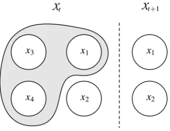
A. Estimation of A 2-D, Homogeneous, Four-State System
Initially a simple spatio–temporal model with two obser-vation locations and four states is used. Fig. 2 represents this graphically where the shaded area describes the neighborhood of . The neighborhood of only contains and -a result of translating the neighborhood down by the spatial distance between and . Following the algorithm given in Table I, this neighborhood generates a transformation matrix
and parameter values are chosen as
The disturbance and noise covariances are chosen to be
and .
Fig. 2. Example neighborhood for Section IV-A. Part of the hidden field is shown for timet + 1, and the whole hidden field is shown for timet. The neighborhood ofx (t + 1)is shown by the shaded region.
Fig. 3. Ten runs of the algorithm using different noise realizations. The figure shows the parameter bias as a percentage of the true-value.
TABLE IV
TRUE ANDESTIMATEDPARAMETERSCORRESPONDING TO
THREECASESSHOWN INFIG. 3
Table IV presents the best, median and the worst parameter es-timates of the 10 runs of the algorithm shown in Fig. 3.
Fig. 4 displays the sensitivity of the parameter estimate to changes in used in the estimator. Here, 100 random matrices were generated by choosing a random matrix via Matlab’s function then setting to en-sure a positive definite covariance matrix. Using the same state sequence, each randomly chosen was presented to the maxi-mization routine (16). This figure demonstrates the insensitivity
[image:8.594.43.290.249.443.2]Fig. 4. Behavior of the maximize routine when presented with randomly chosen covariance matrices but the same data set.
Fig. 5. Example neighborhood for Section IV-B. The neighborhood ofx (t +
1)is shown by the shaded region.
of the algorithm to errors in the state disturbance covariance ma-trix. This is an important numerical property of the estimator, as
may not be well characterized in practice.
B. Estimation of a 2-D, Homogeneous, 12-State System
In order to emphasize the benefits of the neighborhood defini-tion, Table V presents a comparison of the estimation of a stan-dard vector-AR (VAR) model using least-squares with the result using the algorithm of Table III. The system has states, observations locations and a neighborhood definition as shown in Fig. 5. The neighborhood shape is the same for each hidden variable in . The disturbances are the same as for the
previous example where and .
Shown in the table are only the nonzero parameters and their estimates. Here, an estimate for the parameter vector of the VAR model is found using least squares on the original data set without the neighborhood definition and is displayed next to the result using the algorithm given in Table III.
[image:8.594.354.504.296.460.2]Fig. 6. A heterogenous 3-D example. The neighborhood ofx tox is shown left-to-right by the shaded states.
TABLE V
PARAMETERESTIMATES FOR AVAR MODELCOMPAREDWITH THE
SPATIO–TEMPORALMODEL(1)
automatic neighborhood detection is infeasible by naïvely inferring from zero-or small-valued parameter estimates from a nonparameterized system identification procedure.
To demonstrate the effect of the neighborhood mapping on the algorithm, note that the least-squares step applied above is of order and one M-step of Theorem 1 is of order , noting that the product as-sociated with the neighborhood mappings can be considered a sorting operation. The order of the least-squares computation is typically lower, depending on the neighborhood parameteriza-tion. The E-step is typically less complex than the M-step (un-less number of model parameters is significantly reduced by and the observation sequence is either very long or consists of only a small number of observation locations). The complexity of the algorithm increases linearly with the number of iterations. For the example given above, a G4 PowerPC takes s each for the E-step and the M-step, and s for the least squares com-putation.
C. Estimation of a 3-D, Heterogeneous, Eight-State System
A 3-D example is shown in Fig. 6. Here
and the parameters of are given in Table VI. Again, the noise
covariances and . The
neighbor-hood for each hidden variable in is defined separately, rather
TABLE VI
TRUE ANDESTIMATEDVARANDSPATIO–TEMPORALMODEL(1)
PARAMETERS FOR THEHETEROGENEOUS3-D EXAMPLE
than being translated versions of one another, creating a hetero-geneous system whose behavior is dependent on the absolute spatial location. Using the algorithm given in Table I, this neigh-borhood generates a transformation matrix
leaving 18 unknown parameters to be estimated. The algorithm converges in 27 iterations.
The parameter estimates generated are shown in Table VI, compared with the estimated parameters of the VAR model. In this example, the VAR model parameters are estimated using a state sequence that has been smoothed using the true param-eter values. The VAR paramparam-eter estimates still suffer due to the much larger space from which to select the parameter vector. This demonstrates the clear benefit of the model structure via incorporation of the neighborhood definition.
V. CONCLUSION
neighborhood effects the maximum likelihood parameter esti-mation problem and how it improves the modeling accuracy.
The class of model put forward can be considered nonsta-tionary-in-space and stationary-in-time. Both the neighborhood and the associated parameters can be different at different points in the field at a given time, i.e., the homogeneity assumption can be broken without affecting the linearity or Gaussian as-sumptions and, therefore, without affecting the accuracy of the estimator. This class of model is also suitable for modeling pro-cesses observed at locations which are distributed irregularly across space.
The price paid for this flexibility is the potential loss of par-simony and an increase in computational complexity over stan-dard techniques. In applications with a high number of obser-vation locations a different mapping between the observed and hidden fields is required. However, for applications which use a low number of observation locations but which are detailed in time, the neighborhood based spatial time-series model provides a conceptually clear and easily implementable framework. The increase in complexity introduced by the neighborhood map-ping is mitigated by the accuracy of the parameter estimates.
A number of extensions to the presented framework can be considered. A fully heterogeneous system could be modeled by considering nonstationary parameters, which would incorporate the standard Kalman smoother. Attention could also be paid to the parsimony issue; techniques such as making simplifying as-sumptions on the space to be modeled could allow for a greater number of observation locations to be dealt with before having to make the compromise for a more complex model. Finally, as in the coupled map lattice literature [25], the need for a system-atic neighborhood detection scheme is clear, meaning that the neighborhood need not be treated as prior information.
ACKNOWLEDGMENT
The authors would like to acknowledge the anonymous re-viewers for their valuable suggestions.
REFERENCES
[1] J. von Neumann, Theory of Self-Reproducing Automata. Chicago: Univ. Illinois Press, 1966.
[2] K. Kaneko, Ed., Theory and Applications of Coupled Map Lattices. New York: Wiley, 1993.
[3] D. Coca and S. A. Billings, “Analysis and reconstruction of stochastic coupled map lattice models,”Phys. Lett. A, vol. 315, pp. 61–75, 2003. [4] P. C. Kyriakidis and A. G. Journel, “Geostatistical space-time models:
A review,”Math. Geol., vol. 31, no. 6, pp. 651–684, 1999.
[5] P. E. Pfeifer and S. J. Deutsch, “Identification and interpretation of first order space-time ARMA models,”Technometrics, vol. 22, no. 3, pp. 397–408, 1980.
[6] P. E. Pfeifer and S. J. Deutsch, “A three-stage iterative procedure for space-time modeling,”Technometrics, vol. 22, no. 1, pp. 35–47, 1980. [7] D. S. Stoffer, “Estimation and identification of space-time ARMAX models in the presence of missing data,”J. Amer. Statist. Assoc., vol. 81, no. 395, pp. 762–772, 1986.
[8] B. K. Epperson, “Spatial and space-time correlations in ecological models,”Ecolog. Model., vol. 132, pp. 63–76, 2000.
[9] N. Cressie, Statistics for Spatial Data. New York: Wiley, 1993. [10] A. Jenkinson, S. Kadirkamanathan, S. Scott, E. Yazaki, and D. Evans,
“Postoperative factors affecting outcome following laparoscopic fun-doplication for control of acid reflux,”Br. J. Surg., vol. 90, no. 3, pp. 372–373, 2003.
[11] M. A. L. Nicolelis and S. Ribeiroa, “Multielectrode recordings: The next steps,”Curr. Opin. Neurobiol., vol. 12, no. 5, pp. 602–606, Oct. 2002.
[12] R. A. Garrido, “Spatial interaction between the truck flows through the Mexico–Texas border,”Transport. Res. Part A, vol. 34, pp. 23–33, 2000.
[13] R. H. Shumway and D. S. Stoffer, “An approach to time series smoothing and forecasting using the EM algorithm,”J. Time Series Anal., vol. 3, no. 4, pp. 253–264, 1982.
[14] G. A. Smith and A. J. Robinson, A comparison between the EM and subspace identification algorithms for time-invariant linear dynamical systems Cambridge Univ., Eng. Dept., 2000, Tech. Rep..
[15] B. Ninness and S. Gibson, On the relationship between state-space-sub-space-based and maximum-likelihood system identification methods Univ. Newcastle, Australia, 2000, Tech. Rep..
[16] H. E. Rauch, F. Tung, and C. T. Striebel, “Maximum likelihood estimates of linear dynamic systems,” AIAA J., vol. 3, no. 8, pp. 1445–1450, 1965.
[17] T. Gneiting, M. Genton, and P. Guttorp, Geostatistical space-time models, stationarity, separability and full symmetry Univ. Wash., Tech. Rep. 475, 2005.
[18] L. Ljung, System Identification: Theory for the User, 2nd ed. Engle-wood Cliffs, NJ: Prentice-Hall, 1999.
[19] S. Gibson and B. Ninness, “Robust maximum-likelihood estimation of multivariable dynamic systems,”Automatica, vol. 41, pp. 1667–1682, 2005.
[20] W. Steeb, Matrix Calculus and Kronecker Product With Application and C++ Programs. Singapore: World Scientific, 1997.
[21] R. H. Shumway and D. S. Stoffer, Time Series Analysis and Its Appli-cations. New York: Springer, 2000.
[22] K. Xu and C. Wikle, “Estimation of parameterized spatio-temporal dynamic models,”J. Stat. Planning Inference, vol. 137, no. 2, pp. 567–588, 2007.
[23] G. J. McLachlan and T. Krishnan, The EM Algorithm and Exten-sions. New York: Wiley, 1997.
[24] C. F. Wu, “On the convergence properties of the em algorithm,”The Ann. Stat., vol. 11, no. 1, pp. 95–103, 1983.
[25] S. A. Billings and Y. Yang, “Identification of the neighborhood and CA rules from spatio-temporal CA patterns,”IEEE Trans. Syst. Man Cybern. B, vol. 3, no. 2, 2003.
Michael Dewar received the M.Eng. degree in control systems engineering and the Ph.D. degree in systems engineering both from The University of Sheffield, U.K., in 2002 and 2007, respectively.
He is currently working as a Research Associate in the Department of Automatic Control and Systems Engineering, The University of Sheffield. In 2004, he was with the Department of Electrical Power and Control Engineering, University of Malta. His inter-ests surround the modeling of dynamic spatiotem-poral systems, including parameter and state estima-tion for constrained state space models, modeling from irregularly sampled data sets, and the modeling of heterogenous spatiotemporal fields.
Visakan Kadirkamanathan (M’90) received the B.A. and Ph.D. degrees in electrical and information engineering from the University of Cambridge, U.K. He held research associate positions with the Uni-versity of Surrey, U.K. and the UniUni-versity of Cam-bridge before joining the Department of Automatic Control and Systems Engineering, The University of Sheffield, U.K., as a lecturer in 1993. He is currently Professor and is with the Signal Processing and Com-plex Systems Research Group. His research interests include nonlinear signal processing, particle filters, intelligent control, optimization and decision support, swarm intelligence and applications in systems biology, aerospace fault diagnosis, and wireless com-munication signal detection andad hocnetworking. He has coauthored a book on intelligent control and has published more than 110 papers in refereed jour-nals and proceedings of international conferences.
Dr Kadirkamanathan is the coeditor of theInternational Journal of Systems Scienceand has served as an Associate Editor for the IEEE TRANSACTIONS ON
NEURALNETWORKSand the IEEE TRANSACTIONS ONSYSTEMS, MAN,AND