Navigation problems for autonomous robots in distributed environments

(1)

The University of Liverpool

Doctoral Thesis

Navigation Problems for

Autonomous Robots in Distributed

Environments

Author:

Thomas Gorry

Supervisors:

Dr. Russell Martin

Prof. Leszek G¡sieniec

A thesis submitted in fullment of the requirements

for the degree of Doctor of Philosophy

in the

Complexity Theory and Algorithms Group

Department of Computer Science

(2)

Computer science is no more about computers than astronomy is about tele-scopes."

(3)

THE UNIVERSITY OF LIVERPOOL

Abstract

Faculty of Science and Engineering Department of Computer Science

Doctor of Philosophy

Navigation Problems for Autonomous Robots in Distributed Environments

by Thomas Gorry

(4)

Acknowledgements

I would like to express my gratitude to my supervisors, Dr. Russell Martin and Prof. Leszek, whose guidance, knowledge and patience added greatly to my ex-perience as a PhD student. I would also like to thank my academic advisors, Dr. Prudence W.H. Wong, Dr. Martin Gairing and Dr. Igor Potapov for their time and feedback during my studies.

I must also acknowledge all of my co-authors for their contributions to the papers we worked on together. I found these experiences both enjoyable and enlightening.

I would like also to give a very special thanks to my family for the support they provided me, both through my studies and also throughout my entire life. Without their love, encouragement and understanding i would not have nished this thesis.

Finally, in conclusion. I wish to thank all of my colleagues from The Department of Computer Science at The University of Liverpool. I have made some good friends along the way and shared some fun experiences with all of you.

(5)

List of Figures

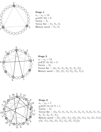
3.1 A simple example of the algorithm at work when n= 27. . . 41

4.1 Time/space diagram for the evacuation procedure in Algorithm 5. . 55

4.2 Time/space diagram of conguration used to establish the lower bound . . . 59

4.3 An optimal strategy for two dierent speeds, where the slower robot has a speed at least 1/3 the speed of the fast robot. . . 64

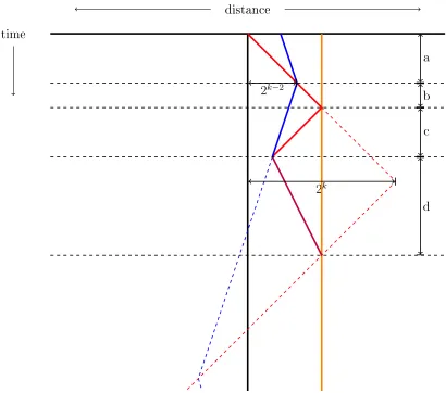
4.4 Example of 9d for evacuation problem, where_SMRhas s _≥ 1 3 and the evacuation point is at2k−2+ε . . . 65

4.5 A strategy for two robots with unit speed and a third robot with speed at least 1/5 the speed of the fast robot. . . 68

5.1 Evacuation of two robots without wireless communication. . . 74

5.2 Forming a square ABCD of positions not yet explored by the robots. 76 5.3 Evacuation of two robots with wireless communication. . . 78

5.4 Construction of sets L and R. . . 79

5.5 Evacuation of three robots with wireless communication. . . 84

5.6 k robots with wireless communication . . . 88

(10)

(11)

List of Algorithms

1 The location-discovery procedure of a robot. . . 28

2 FasterDiscovery(n: integer) . . . 39

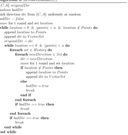
3 IncreaseGranularity() . . . 40

4 A doubling strategy for a single mobile robot . . . 52

5 Coordinated evacuation for two mobile robots on the line . . . 54

6 Algorithm for two robots without wireless communication. . . 74

7 Algorithm for two robots with wireless communication. . . 78

8 Algorithm for three robots with wireless communication. . . 84

9 Algorithm for k robots without wireless communication. . . 87

10 Algorithm fork robots with wireless communication. . . 89

(12)

(13)

List of Tables

1.1 Examples of asymptotic notations and their meanings. . . 3

2.1 The author's publications and co-authors throughout the duration of the author's PhD studies. . . 17

5.1 Upper and Lower bounds for k _≥2 robots . . . 73

(14)

(15)

Abbreviations

i If and only IF

w.h.p. With High Probability

M E Mobile Entity

MR Mobile Robot FMR Fast Mobile Robot SMR Slow Mobile Robot s.t Such That

CCP Coupon Collectors Problem

(16)

(17)

Dedicated to my parents, Tom and Liz, and my sister

Joanne.

We all have dreams but in order to make those dreams

into a reality it takes the support from a loving family.

(18)

(19)

Chapter 1 Preface

1.1 Algorithms

This Chapter has been included for readers who are perhaps unfamiliar with the topic of this work. In this section the concept of algorithms will be introduced along with explanations of what it means to analyse them as well as some technical explanation.

1.1.1 Overview

Algorithms are procedures used to solve some task. More specically, they are well dened steps that take an input either as a single value or a set of values and then outputs either a single value or a set of values. In this way algorithms can be seen as a sequence that can be followed to solve a computation problem.

1.1.2 Analysis

When we talk about analysing an algorithm quite often we are measuring its eciency in some way. The metric of eciency for an algorithm is usually based on its speed. However, one could just as easily measure its memory or energy usage as a metric for analytical purposes.

We live in a world where there are still many problems we do not even know exist, let alone are aware of ecient solutions to them. However, for thoes problems

(20)

Chapter 1. Preface 2

that we are aware of but have yet to solve them eciently we place into a subset of problems called NP-complete. It is interesting to note that there is a special property that holds for these types of problems that means if an ecient solution is found for one then that means there must also be ecient solutions for the other problems in this subset. Unfortunately, no ecient solution has yet been found for any of these problems. However, in the meantime we can use what we call approximation algorithms to get close to an ecient solution in these cases.

Denition 1.1. running time: The time it takes an algorithm to complete its steps and nish a task.

Denition 1.2. steps: it is assumed that each line of code in an algorithm is a step and that a step will take a constant time to run. That way when comparing algorithms between dierent computers we can still get a reliable measurement on its running time.

For this work we will be interested in the speed of an algorithm, that is the running time that an algorithm needs to complete the given task. Given that depending on what computer an algorithm is run on it may run faster or slower in comparison with the same algorithm on another computer, due to possibly dierent hardware congurations, we measure this running time in the number of steps executed. Furthermore, in order to understand better the performance of an algorithm for any size input we tend to express the running time of an algorithm as a function of n, f(n), wheren is the input size.

Following on from this it is also important to understand that for large values ofn

the lower order terms of the running time function are rendered inconsequential. Therefore, when looking at the running time of an algorithm it is usual to only consider non-constant factors. At this point we are considering the order of growth of the algorithm.

Denition 1.3. order of growth: The rate at which the number of steps an algorithm must perform to reach a solution that is given by the dominant factor in the growth function.

(21)

[image:21.596.104.534.160.418.2]

through asymptotic notation. Table 1.1 shows common examples and denitions of this form of notation.

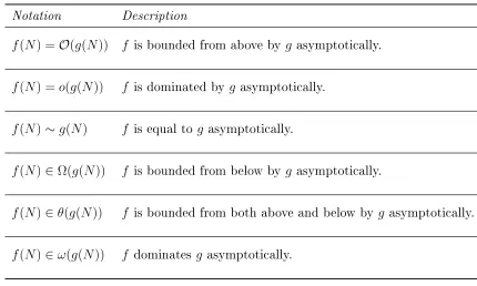
Table 1.1: Examples of asymptotic notations and their meanings.

Notation Description

f(N) = _O(g(N)) f is bounded from above by g asymptotically. f(N) = o(g(N)) f is dominated by g asymptotically.

f(N)_∼g(N) f is equal to g asymptotically.

f(N)_∈Ω(g(N)) f is bounded from below by g asymptotically.

f(N)_∈θ(g(N)) f is bounded from both above and below by g asymptotically. f(N)_∈ω(g(N)) f dominates g asymptotically.

1.2 Distributed Computing

This thesis has its roots rmly embedded in Distributed Computing, that is com-puting that takes place in a Distributed Setting.

Denition 1.4. Distributed Setting: A setting that has no central or controlling aspect. In computing this can be seen as groups of networked computers that have processors running concurrently in parallel, each with its own memory.

Distributed Computing tackles problems by utilising the collective power of the computers or, in the case of this work, robots that inhabit the system. The algo-rithms in this work therefore are part of a category of algoalgo-rithms called Distributed Algorithms. Quite often Distributed Algorithms will tackle separate parts of the problem with information spread across the system.

(22)

One of the biggest factors for Distributed Algorithms is the coordination of the processors involved in solving the task. However, there are huge benets to using Distributed Algorithms in the correct setting. For example, a good Distributed Algorithm will allow for better levels of fault tolerance than a traditional algorithm as the other processors in the system should seamlessly pick up where the failed one left of. Furthermore, often it is the case that by splitting a task into sub-parts that can be carried out by each processor, or robot, in the system the task can be completed much faster.

1.3 Specic Chapter Denitions

This section of the chapter is designed to layout some specic denitions of notions that will be used later on in this work.

1.3.1 Location Discovery

The following denitions are in reference to Chapter 3.

Denition 1.6. Arbitrary but distinct positions: What is meant here is that each robot starts at a position that is randomly determined and is independent from the other robots starting locations.

Denition 1.7. Unit Circle: A unit circle usually means a circle with a radius of 1. However, for the purpose of Chapter 3 we talk of a unit circle having the

circumference of 1. This is done without loss of precision as it simply allows us to

normalise things with respect to1, thereby making explanations and

understand-ings clearer.

Denition 1.8. Anonymous Robots: Robots are dened as anonymous as they are unknown to one another and given their starting conguration there are no fundamental dierences between them and so they could be interchanged without impact.

(23)

Denition 1.10. Synchronised Rounds: The notion of synchronised rounds sim-ply referes to the fact that all rounds are performed by the robots at the same time and at the same pace.

Denition 1.11. Leaving marks: When we refer to robots leaving marks it is to be understood that for a robot to leave a mark this could mean that they can leave some sort of signal or note for either other robots, or itself, to discover and use at a later date.

Denition 1.12. Exchanging messages: Robots exchanging messages simply refers to communication between robots. However, in Chapter 3 the robots are limited to no communication with one another outside of collisions that occur during the walking phase of a round.

Denition 1.13. Coupon Collector's Problem (CCP): One player must collect m

coupons. During each consecutive attempt the player draws each coupon with probability 1

m. One can use a short calculation and a union bound to prove that

after α _·mlogm attempts the player is left without a full set of coupons with

probability at most 1

mα−1, for any constant α >1[98]. CCP can be also executed

in consecutive stages, where each stage can be formed of a xed number ` of

consecutive attempts. In this case one can conclude that it is enough to run

α_· m

` logm stages to collect all coupons with high probability 1−1/m α−1.

1.3.2 Evacuation Problem

The following denitions are in reference to Chapter 4 and Chapter 5.

Denition 1.14. Group Search: In this context Group Search is the type of problem we have carried out research on. It involves a group of robots searching for one or more locations or another robot or other robots in a given environment. In this work we look at the Evacuation Problem. This is a form of group search problem where one or more robots search for a location from which to evacuate the environment. The task is complete when all of the robots in the system have reached that location.

(24)

Denition 1.16. Disk: In Chapter 5 we consider the environment of a disk. This disk is a unit disk where the radius of the disk is 1. The robots start o in

the centre of the disk and are tasked with locating a single point that is on the perimeter of that disk.

Denition 1.17. Mobile Robots: For the purpose of this work all robots men-tioned have the ability to move and there should be no distinction between the use of "robots" and "mobile robots".

Denition 1.18. Maximal Speed: The maximal speed of a robot is the fastest speed that the robot is able to travel by.

Denition 1.19. Unit Speed: Throughout this work we make explanation and understanding clearer by designating the maximal speeds of the robots to be that of a unit speed. A unit speed in this context simply means a speed= 1.

Denition 1.20. Non-Wireless/Local Communication: When we talk about non-wireless or local communication what is meant is that the robots are only able to communicate with one another when they occupy the same location. We assume that communication happens instantly and that there is no chance of missed or corrupt communication occurring.

(25)

Chapter 2 Introduction

2.1 Motivation and Problem Scope

This thesis looks at the area of Distributed Algorithms in the eld of Computer Science, more specically it investigates the area of Control Problems for Mobile robots in Distributed Settings. Work carried out on applied areas of Graph Theory and Network Analysis can also be found within this thesis.

Firstly, however, we will talk about the world of Mobile robots. The trends in processing power described by Moore's law and the trends in network trac are increasing at dierent rates and so the power of our processors cannot keep up with the demand placed on our networks today. With that said, there is therefore a need for Distributed Computing, and that will increase further with large parts of the developing world set to be fully connected to the Internet and thus the Cloud in the near future. This would suggest that the future of computing will be heavily dependent on solutions that are, at the very least in part, distributed.

Already the move towards a distributed world has begun with huge leaps forward in the past few years with regards to making use of distributed computing solutions in our daily lives. There has been work done by [95] with the aim of creating a self-organising group of robots to build structures. They work in a scenario where the robots must locate the building blocks needed and then move the blocks into position to create a useful structure. The approach used is an increasingly popular one of looking to nature for the solution with a biological-inspired swarm intelligence based algorithm proposed.

(26)

Chapter 2. Introduction 8

There has been much talk about using teams of robotic swarms to explore planets that are incapable of supporting life and would provide a much cheaper option than sending a team of astronauts to these planets themselves. [108] propose an autonomous robotic swarm exploration to search for extra-terrestrial life on Mars. This would also have applications in a military sense where it may be too dangerous to send humans in to do reconnaissance, intrusion detection or mine clearing [110].

Leading on from the dangerous settings of the area of war, there has been sig-nicant strides in multi-robot teams for Search and Rescue situations in natural disaster zones [24, 91]. [24], for example, introduce a multi-robot algorithm for the use in search and rescue scenarios for exploration of unknown terrain. Their solution allows for parallel search and rescue operations to be run alongside each other by exploiting the robustness of distributed teams of robots.

Looking more towards the industrial front and how distributed computing can be used to enhance our economic needs [48, 76, 88, 101]. Perhaps the most famous example of this would be the success story of Kiva Systems, [114], who are now owned by Amazon and have developed and continue research on teams of mobile robots that manage the giant warehouses that house the stock sold on the online market site. The work done in [48, 76, 88] shows how swarms of small automated guided vehicles are employed to collect items from storage shelves in warehouses and take them to a picking station that helps to simultaneously improve produc-tivity and speed. In this way operators are able to simply stand still and have the required move towards them. This method employs the use of inventory pods that are picked up and moved by hundreds of mobile robot platforms. In 2009 the largest number of Kiva robots in a single warehouse stood at 500, [93], for a supply company in the USA. Since Amazon integrated the company into their business that record has been smashed with Amazon itself having 15,000 Kiva robots spread across its 10 main warehouses in their network, [38].

(27)

As it is plainly evident from the applications mentioned above this area of comput-ing, although studied now for several years, can only continue to grow in number of applications and importance in humanities dependency upon such systems. This is why it is imperative that we grow our understanding of the mechanisms and strategies that control and govern the movements of such Mobile Entities, MEs, so that we are able to keep up with the demand for ever more intelligent and dynamic solutions based upon a distributed approach to problem solving in todays modern world.

2.2 Background

2.2.1 Search and Discovery Problems

The Search Problem is well-studied within the elds of operations research, com-puting, and mathematics. This problem deals with a searcher looking for a hidden object (or target), wishing to minimize a resource used in nding it. Many ver-sions of this problem can be considered, including variations in the environment, whether the target is xed or mobile, and, the use of a deterministic or random-ized search strategy. Furthermore, there can be dierences in the approach con-sidered with respect to the resource being minimised. There has been much work done with respect to minimising the time to nd the target [79, 13, 14, 27, 32 34, 43, 46, 47, 50, 52, 78] as well as minimising the memory used to nd the tar-get [56, 73]. In the context of search and discovery of dierent varieties of environ-ments there is a large volume of robot network exploration algorithms, they mainly focus on network topology discovery either in graph-based networks [27, 32, 41, 67] or in geometric setting [43, 52, 78, 115].

(28)

approach as in [27, 32, 34, 46, 67, 68, 73, 105, 115]. There are many advantages that endorse the use of distributed mobile systems. Working together the MEs can not only increase their eciency but also their reliability through redundancy. Furthermore, the cost of such MEs is reduced through being able to use less advanced MEs to complete the same tasks, either through things like reduced memory or energy used.

However, having MEs that are less advanced sometimes presents its own problems. For example, sometimes it is necessary for the MEs to perform a distributed task without all performing exactly the same set of commands. If there exists no way to communicate or identify the MEs from one another what can be done to break the symmetry? In this case we move away from deterministic approaches of addressing these problems and look towards randomisation for the solution as done in [54, 68].

Search and Discovery problems can also inherently be seen as types of control problems and as with other control problems many have looked towards the nat-ural world to help come up with innovative algorithmic solutions, some based on Brownian Walks and Levy Flights [107, 119] and others looking towards the insect world with ant and bee colony mechanisms [49, 58, 117].

As seen from above there can be many variations on the Search and Discovery problem and the book by Alpern and Gal [8] is a good survey of known results for these.

2.2.2 Rendezvous and Gathering Problems

Search Problems also naturally lead into the Rendezvous Problem, where two or more searchers seek to meet in an environment, and this problem naturally lends itself to additional considerations of the inherent abilities of the searchers them-selves, such as whether they have the same speed or dierent speeds, their ability to communicate and see (typically over a limited distance), and if the searchers are able to follow the same or dierent search strategy (e.g. do the searchers have unique identiers so they can adopt their own search method, or are they in-distinguishable and therefore must use the same (randomized or deterministic) strategy?).

(29)

the distributed side the main problem that is obvious is agreeing upon a place to meet. This of course can be made more dicult by limitations on communication. As mentioned earlier Rendezvous and Gathering Problems tend to lead on from Search Problems meaning that many of the variations studied above also apply here with a lot of research being done in a variety of settings and with a variety of constraints [37, 84, 100, 113]

2.2.3 Monitoring and Patrolling Problems

The Monitoring Problem is where, in a graph or geometric environment (such as a simple polygon), MEs are arranged in stationary positions to constantly survey the graph or region and usually the MEs have a limited eld of vision. One of the main targets of such problems is to maxamise the visual range with the minimum number of MEs as there is probably a cost for each additional ME introduced into the system. This formulation of the problem is known widely as the Art Gallery Problem [36].

The problem has gained much popularity in recent years, [21, 59, 71, 121] with the emergence of more advanced robotic systems meaning that truly distributed structures can be deployed easily. The idea of MEs that are able to self-organise into a suitable conguration for ecient monitoring has been looked at by [121] in relation to vehicles that can communicate with each other to position themselves eectively on road systems to minimise congestion with reduced impact on travel time. Also [59] has looked into neighbour discovery in a sensor network with directional antennae.

(30)

It is worth noting here that in the setting of a general graph with edges of equal length then the Network Patrolling Problem is NP-Hard as if there exists only a single ME then the problem becomes one of nding a Hamiltonian cycle in the graph, [29].

As with the previous problems looked at in this chapter the Network Patrolling Problem is also subject to a wide variety of settings and constraints that can be imposed to make the problem more realistic to the real world or more interesting to study. For example, [3] uses a model where communication between the MEs is limited. This adds an extra dimension of complexity to the problem and can be used to accurately model a real world situation where surveillance is being performed where radio silence is necessary.

Furthermore, just like with the Search Problem it may be benecial to break up the symmetry of a deterministic approach by adopting a randomised algorithm instead when patrolling [4, 69, 106]. Although, this time the breaking of symmetry may be simply to enable more ecient paroling in terms of attempting to fool any potential intruders. A Bayesian learning method was used by [106] to do just this.

The Network Paroling Problem has many real world applications. One of which is an intuitive jump to make from theoretical surveillance to that of Unmanned Aircraft Surveillance where work has already been done with that exact scenario in mind [2].

Again nature can also help provide useful solutions to problems with work being done using strategies taken from ant colonies to enable paroling of areas or net-works based on the pheromones left behind to help ensure portions of the patrolled locations do not go untended for too long [69].

2.3 Summary of Results

2.3.1 Robot Location Discovery

The results we obtained in this area have been published in [68] and are presented in full in Chapter 3. What is presented is a randomised distributed communication-less coordination mechanism for n uniform anonymous robots located on a circle

(31)

on the ring, unknown to other robots. The robots perform actions in synchronised rounds. At the start of each round every robot chooses the direction of its move-ment (clockwise or anticlockwise), and moves at unit speed during that round. Robots are not allowed to pass by one another, i.e., when a robot collides with another it instantly starts moving with the same speed in the opposite direction. Robots are also unable to leave marks on the ring, have zero vision and cannot exchange messages. However, on the conclusion of each round each robot obtains (some, not necessarily all) information regarding its trajectory during this round and no other. This information can be processed and stored by the robot for further analysis.

The Location Discovery Task to be performed by each robot is to determine the initial position of every other robot in the system at the start of the scenario and eventually to return and stop at its own initial position, or proceed to another task such as Boundary Patrolling, in a fully synchronised manner. The primary motivation was to study distributed systems where robots collect the minimum amount of information that is necessary to accomplish this location discovery task.

Our original result for this problem was a fully distributed randomised (Las Vegas type, [16]) algorithm, solving the Location Discovery Task w.h.p. in O(nlog2n)

rounds (assuming the robots collect sucient information). Note that this result also holds if initially the robots do not know the value of n and they have no

coherent sense of direction. We believe that our work in [68] is the rst attempt to solve the distributed boundary patrolling problem in the geometric ring (circle) model. Furthermore, the proof technique of the concept of virtual "batons" that robots exchange with each other upon collision, we believe, is a novel and intriguing approach to analysing the motion of the robots in the system. To our knowledge this is the rst time such an approach has been used to analyse such a system and it led to us discovering a rotation of robots positions at the end of each round. This in turn had a large impact on us designing and analysisng the resulting algorithm. This method has since been explored and built upon by [45] and [44].

However, Chapter 3 presents another fully distributed randomised (Las Vegas type, [16]) algorithm that can achieve success w.h.p signicantly faster in n +

O(log2n) rounds. Given the constraints of the model any algorithm will need

to visit all n locations anyway and so there is no escaping this cost. Following

(32)

belief that this new algorithm is in fact the optimal solution for this problem as our approach works by each robot remembering not only where they have been but the decisions it made to get there. This allows the robot to remember any benecial decisions and reapply them throughout the process while at the same time avoiding repeating any costs. However, we have yet to formalise a proof for this claim.

2.3.2 Evacuation Problem on the Line

The results we obtained for the Evacuation Problem on the Line have been pub-lished in [34] and are presented in full in Chapter 4.

We consider the Group Search Problem on the Line, or Evacuation Problem on the Line, in whichkrobots located on the line perform search for a specic destination.

The robots are initially placed at the same point (origin) on the line L and the

target is located at unknown distance d either to the left or to the right from the

origin. All robots must simultaneously occupy the destination, and the goal is to minimize the time necessary for this to happen. The problem withk = 1is known

as the Cow Path Problem, and the complexity of this problem is known to be9din

the worst case (when the cow moves at unit speed), wheredis the distance between

the origin and the destination. It is also known that this is the case fork≥1

unit-speed robots. Our results show for the rst time a clear argument for this claim by showing a rather counter-intuitive result. Namely, in any metric, independently from the number of robots, group search cannot be performed faster than in time

9d. We also examine the case of k = 2 robots with dierent speeds, showing a

surprising result that the bound of 9d can be achieved when one robot has unit

speed, and the other robot can move with speed at least 1

3. Finally the case where

k = 3 robots, with one having a speed less than 1, is briey looked at and we

show that a bound of 9d can yet again be achieved, but only if the slower robot's

speed is at least 1

(33)

2.3.3 Evacuation Problem on the Disk

Our work on the Evacuation Problem on the Disk has been published in [46] and is presented in full in Chapter 5 of this thesis.

In this work k mobile robots inside a circular disk of unit radius are considered.

The robots are required to evacuate the disk through an unknown exit point situated on its boundary. It is assumed all robots have the same (unit) maximal speed and start at the centre of the disk. The robots may communicate in order to inform each other about the presence (and its position) or the absence of an exit. The goal is for all the robots to evacuate through the exit in the minimum time possible.

Two models of communication between the robots were considered: In non-wireless (or local) communication model robots exchange information only when simulta-neously located at the same point, and wireless communication in which robots can communicate between each other at any time.

The following question for dierent values of k is studied: What is the optimal

evacuation time fork robots? We were able to construct algorithms to accomplish

this and present lower bounds in both communication models fork= 2 and k= 3

thus indicating a dierence in evacuation time between the two models. Almost-tight bounds are also obtained on the asymptotic relation between evacuation time and team size, for largek. Also in the local communication model it is shown

that, a team of k robots can always evacuate in time 3 + 2_kπ, whereas at least 3 +2_kπ₋O(k−2₎time is sometimes required. In the wireless communication model, time 3 + π_k +O(k−4/3₎ _{always suces to complete evacuation, and at least} _{3 +}π

k

is sometimes required. This shows a clear separation between the local and the wireless communication models.

We found that one of the remarkable points of interest for this problem was that when increasing the number of participating robots only slightly, and still when considering a relativity small number of k, the compexity of the problem itself

(34)

2.4 Thesis Structure

The chapters in this thesis contain both work related to the main topic of the doctorate as well as several side interests that the author has pursued throughout its duration. The material covered in this thesis has been aranged in the following way:

Chapter 3

This chapter covers Search and Discovery problems, going into the back-ground of the topic as well as presenting results obtained in [68], as well as progress made that expands upon this work.

Chapter 4

The material in this chapter focuses more on the collaboration of MEs to achieve goals while still in the context of Search and Discovery problems as well as introducing The Evacuation Problem and the results relating to this produced in [34].

Chapter 5

Expanding on the previous chapter, here details of the material presented in [46] as an obvious path forward following the promising work accomplished in [34] will be discussed.

Chapter 6

The nal chapter shows the conclusions of this work and looks further av-enues forward for this research.

2.5 Author's Contribution

(35)

[image:35.596.141.494.178.440.2]

Everything else is the author's work, written for this PhD project and supervised by Russell Martin and Leszek G¡sieniec.

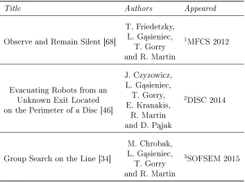
Table 2.1: The author's publications and co-authors throughout the duration of the author's PhD studies.

Title Authors Appeared

Observe and Remain Silent [68]

T. Friedetzky, L. G¡sieniec,

T. Gorry and R. Martin

1_{MFCS 2012}

Evacuating Robots from an Unknown Exit Located on the Perimeter of a Disc [46]

J. Czyzowicz, L. G¡sieniec,

T. Gorry, E. Kranakis,

R. Martin and D. P¡jak

2_{DISC 2014}

Group Search on the Line [34]

M. Chrobak, L. G¡sieniec,

T. Gorry and R. Martin

3_{SOFSEM 2015}

4_{MFCS 2012: The 37th International Symposium on Mathematical Foundations}

of Computer Science, 2012

5_{DISC 2014: The 28th International Symposium on Distributed Computing, 2014.}

6_{SOFSEM 2015: 41st International Conference on Current Trends in Theory and}

(36)

(37)

Chapter 3 Location Discovery

3.1 Introduction

This chapter is based heavily on results published in [68] at The 37th Interna-tional Symposium on Mathematical Foundations of Computer Science in 2012 (MFCS'12). There is also work presented in this chapter concerning improvements to the location discovery problem presented in [68] that have been discussed

be-tween the author and their supervisors but at the time of writing have still yet to be published. Furthermore, it should be noted here that the initial idea for this problem and the beginnings of the initial solution are already part of the author's Master's Dissertation, [75], but have been included here as they provide the foun-dations for what eventually became the paper we published that was mentioned at the start of this paragraph, [68].

In this chapter we study a randomised distributed communication-less coordina-tion mechanism for n uniform anonymous robots located on a circle with unit

cir-cumference. We assume the robots are located at arbitrary but distinct positions, unknown to other robots. The robots perform actions in synchronised rounds. At the start of each round a robot chooses the direction of its movement (clockwise

oranti−clockwise) and moves at unit speed during this round. Robots are not

al-lowed to overpass,i.ewhen a robot collides with another it instantly starts moving

with the same speed in the opposite direction. Robots cannot leave marks on the ring, have zero vision and cannot exchange messages. However, on the conclusion of each round each robot has access to, some (not necessarily all), information

(38)

Chapter 3. Location Discovery 20

regarding its trajectory during this round. This information can be processed and stored by the robot for further analysis.

The location discovery task to be performed by each robot is to determine the initial position of every other robot and eventually to stop at its initial position, or proceed to another task, in a fully synchronised manner. Our primary motiva-tion is to study distributed systems where robots collect the minimum amount of information that is necessary to accomplish this location discovery task.

Our original result for this problem, [68], was a fully distributed randomised (Las Vegas type, [16]) algorithm solving the location discovery problem w.h.p. in O(nlog2n) rounds (assuming the robots collect sucient information). Note

that our result also holds if initially the robots do not know the value ofnand they

have no coherent sense of direction. However, this chapter also presents another fully distributed randomised, Las Vegas type, algorithm that can achieve success w.h.p. signicantly faster in n+O(log2n) rounds.

3.1.1 Overview

(39)

this instance. Numerous algorithms have been developed in the literature for a variety of control problems for robot swarms, see [15, 37, 63, 64, 84, 112]. Most of these algorithmic solutions, with certain exceptions, e.g., [39], impose on the participating robots access to the global picture, in other words the ability to monitor performance of all robots. While there is a large volume of robot network exploration algorithms, they mainly focus on network topology discovery either in graph-based networks [27, 32, 41, 67] or in geometric setting [43, 52, 78, 115]. As mentioned earlier here the focus is on the network model similar to [15] in which communication is limited to a bare minimum. In such networks, the communica-tion deciency of a robot is compensated by an astute observacommunica-tion and analysis of its own movement. The trajectory of a robot's movement in a given round is represented as a continuous, rectiable curve, that connects the start and the end points of the route adopted by the robot. While moving along their trajectories, robots collide with their immediate neighbours, and information on the exact lo-cation of those collisions might be recorded and further processed. When robots are located on a circle, thanks to its closed topology, each robot may eventually conclude on the relative location of all robots' initial positions, even given only limited information about its trajectory. This procedure, in turn, enables other distributed mechanisms based on full synchronisation including equidistant distri-bution along the circumference and optimal boundary patrolling scheme. Most of the models adopted in the literature on swarms assume that the robots are either almost or entirely oblivious, i.e., throughout the computation process the robots follow a very simple, rarely amendable, routine of actions. Oblivious algorithms have many advantages including striking simplicity and self-stabilisation [57] prop-erties.

3.1.2 The Model

In this chapter geometric network model, i.e., a circle with circumference one is adopted, along which a number of robots move and interact in fully synchronised rounds (each of which lasts one unit of time). The robots are uniform and anony-mous to one another. Moreover, the robots do not necessarily share the same sense of direction, i.e., while each robot distinguishes between its own clockwise (C) and anticlockwise (A) directions, robots may not have a coherent view on

(40)

chooses a direction of its move from {A, C_} and moves at unit speed. It is

as-sumed that robots are not allowed to pass over each other along the circle. In particular, when a robot collides with another (robot) it instantly starts moving with the same speed but in the opposite direction. The robots cannot leave marks on the ring, they have zero visibility and cannot exchange messages. Instead, on the conclusion of each round every robot learns a specic information concerning its recent trajectory. In particular, for odd n we assume that a robot is informed

about the relative distance between its location at the start and the end of this round. For evenn,however, the robots must also learn about the exact time

(loca-tion) of their rst collisions during this round. This information can be processed or stored for further analysis. The aim of a robot is to discover the initial posi-tions of all other robots. Our main motivation for [68] was to study distributed systems where robots collect the minimum amount of information necessary to accomplish the location discovery task, and the novelty comes from considering the situation where robots operate with a very limited amount of information col-lected during the discovery procedure. One might consider, for example, that a robot spends energy to determine its current location, and wants to minimize its energy expenditure.

Since the robots never pass over one another it can be assumed that the robots are arranged in an implicit (i.e., never disclosed to the robots) periodic order s.t

robots are located at random intervals along the circumference of the ring from a0 toan−1. The original positions of ai, are denoted by pi for all i∈[n]1. Note that, due to the periodic order of robots, all calculations on implicit labels of robots that follow are performed modulo n.

Note however, that the circumference of the circle has to be known in advance. Otherwise, a participating robot might not be able to tell the dierence between

n= 1 and n >1. In particular, if the robot imposed a limit on the traversal time

until the rst collision, the adversary would always choose the circumference to be large enough to accommodate distant locations between the robots preventing them from ever getting close enough. On the other hand, if the robot continues its search indenitely, the adversary could choose n = 1 and the location

dis-covery process would never end. Thus, it is important to know either n or the

circumference of the circle.

(41)

3.1.3 Results

We assume that n mobile robots are initially located on a circle at arbitrary,

distinct and undisclosed positions. As stated previously, the task of each robot is to determine the initial position of every other robot. On the conclusion of the algorithm robots either synchronously stop at their initial positions or may proceed with another task. For the clarity of presentation, we rst provide a solution to the distributed location discovery under the assumption that the robots have a coherent sense of direction, i.e. they all have the same understanding of what direction clockwise and anti-clockwise is, and the value n is known in advance

to all robots. Later, in Sections 3.3.3 and 3.3.4 we provide further evidence on how these two assumptions can be dropped. Finally, we briey describe how the location-discovery mechanism can be used to coordinate actions of robots in distributed boundary patrolling on circles, see Section 3.3.5. This last part should be seen as a natural continuation of [42] devoted to ecient centralised patrolling mechanisms designed for robots with distinct maximum speeds. We believe that our work in [68] is the rst attempt to solve the distributed boundary patrolling problem in the geometric ring (circle) model. Our work in this chapter shows that we can accomplish this task inO(nlog2n) rounds w.h.p.. However, we

can introduce the concept of a Stationary choice of movement where that robot

initially chooses not to move but instead remains at its starting location until a collision with another robot. Using this we also show in this chapter that with the added inclusion of a Stationary choice of movement at the start of a round

robots are able to accomplish the task w.h.p. signicantly faster in n+O(log2n)

rounds..

All of the bounds in this chapter hold with high probability2 _{(w.h.p.) for} _n _large

enough. However, one can easily modify the solutions such that by periodically repeating actions of robots, they can solve the task with the required level of condence even for smaller, e.g., constant values of n.

3.2 Rotation mechanism

The location-discovery algorithm is formed of a number of stages. Each stage is a sequence of at most n consecutive rounds, each of unit duration. Recalling from

(42)

earlier, a round lasts exactly one unit of time. Given that the ring is one of unit circumference this would be exactly enough time for the robot to walk the entire circumference and arrive back at its original starting location if it experienced no collisions along the way, i.e. if the robot was the only one in the system. At the beginning of the rst round of each stage a robot ai randomly chooses

the direction (clockwise or anticlockwise) of its movement, and moves with unit speed throughout the entire stage. Later throughout the same stage, the exact location and the movement direction ofai depends solely on the collisions with its

neighbours ai−1 and ai+1. We show that on conclusion of each round the robots always reside at the initial positions p0, . . . , pn−1, where there is a k ∈ [n], equal for all robots, such that the current location of robot ai corresponds to pi+k. It

should be noted here that depending on the initial choices of all the robots in terms of their direction of movement then pi+k could also be pi−k. Also note that

this observation allows robots to visit (and record) the initial positions of other robots. Thus, part of the limited amount of information that a robot obtains is its position, relative to its initial starting location, at the end of each round. A stage concludes at the end of a round when each robot ai arrives at its original

starting position pi. We show that w.h.p. robots requireO(log2n) stages to learn

the locations of their counterparts. Since each stage is formed of at mostnrounds,

the total complexity of our algorithms is bounded by O(nlog2n).

Throughout the discovery procedure, robots move with uniform speed one. Recall when two robots collide, they instantly bounce back without changing their uni-form unit speed. While observing two indistinguishable colliding robots, one could wrongly conclude that the two robots overpass each other. We assume that at the beginning of each stage of our algorithm every robotaiholds a unique virtual baton bi. During the rst collision with eitherai−1 orai+1 this baton gets exchanged for a baton currently held by the respective robot. In due course, further exchanges of batons take place. We emphasize that the concept of batons is solely a proof device in what follows, that they do not actually exist as far as the robots are concerned, and that no actual communication (or exchange of any object) takes place between the robots when they collide.

Lemma 3.1. At the start of each round baton bi resides at position pi, for all i_∈[n].

Proof. At the start of the location discovery procedure, bi resides at pi for all i.

(43)

(being exchanged as appropriate during collisions), so bi must arrive at pi on the

conclusion of this rst round. Inductively, at the end of each round (i.e. start of the next round) of the procedure, bi will reside at position pi.

Using Lemma 3.1 it can be concluded that at the start of each round the robots populate initial locations p0, . . . , pn−1. In fact, one can state a more accurate lemma.

Lemma 3.2. There is a k _∈ [n] s.t. at the start of each round, for all i _∈ [n],

robot ai resides at position pi+k.

Proof. At the start of the location discovery procedure, all initial positions are populated by the robots, each carrying a (virtual) baton. From Lemma 3.1, bi

begins (and ends) each round at position pi. Since some robot must always be

carryingbi, there is a robot occupying the locationpi at the beginning of a round,

and some (possibly dierent) robot occupying pi (and holding bi) at the end of

the round. The same argument holds for each i, hence all n initial locations are

occupied at the end (start) of each round. Recall that the robots never overpass, i.e., robot ai always has the same neighbours ai−1 and ai+1. Thus, ifai resides at positionpi+k for somek, then ai−1 andai+1 must reside at the respective locations

pi+k−1 and pi+k+1.

Using the observation from Lemma 3.2, consider the respective locations pj+k1

and pj+k2 of robot ai at the start of two consecutive rounds. One can conclude

that during one round all robots rotated along the initial positions by a rotation index of r=k2−k1, i.e. each robot experiences the same shift by r places (either clockwise or anticlockwise) between the beginning and the end of one round.

Lemma 3.3. During one stage the rotation index r remains unchanged.

(44)

of the batons during the entire stage, i.e. if robot ai chooses clockwise, then

baton bi will move clockwise during that entire stage. Since at the beginning of

each round, the virtual batons reside in their original positions (Lemma 3.1), and they don't change their directions during the entire stage, this means the pattern of movement and collisions (swaps of batons) of the robot beginning a round atpi

will be identical that of ai during the rst round of the stage. Hence, the rotation

index remains unchanged during an entire stage.

Following on from this it can now be shown that the rotation index r depends

on the initial choice of random directions adopted by the robots. Consider the rst round of any stage. Let setsBC andBAcontain the virtual batons that move

during this round in the clockwise and anticlockwise directions, respectively, where

|BC| = nc, |BA| = na, and nc+na = n. We say that during this stage virtual

batons form a (nc, na)-conguration.

Lemma 3.4. In a stage with a (nc, na)-conguration, the rotation index

r=nc₋na.

Proof. By Lemma 3.2 it is enough to prove the premise of the lemma for one robot. Without loss of generality, assume that batonbi is inBC. At the beginning of any

round baton bi is aligned with position pi, and assume that at the beginning of

the considered round bi is carried by robot aj.

First note that bi can only be exchanged with batons from BA since all batons in BC move with the same speed in the clockwise direction. Moreover, during any

round every baton fromBC is exchanged with every baton fromBA exactly twice

at certain antipodal points of the ring. Why is this? Suppose bk _∈BA, and let d

denote the distance (along the circumference) betweenbi and bk, measured in the

clockwise direction. Note thatd <1since robots start at distinct locations. Then

bi and bj meet (are exchanged by colliding robots) at time d/2. After additional

time 1/2 (since d/2 + 1/2 < 1), bi and bk meet again at the antipodal point of

their rst collision before returning to their respective positions atpi and pk.

Thus, during any round baton bi is exchanged between colliding robots exactly

2na times. Also, since bi moves in the clockwise direction during each exchange,

(45)

Focusing on batons from BA, one can use an analogous argument to prove the

rotation factor r = 2nc. Now since nc+na = n it follows that ₋na =nc(mod n)

and nally−2na= 2nc(mod n) admitting the uniform rotation index r across all

robots.

Finally, na+nc (that has value 0 modulo n) is added to ₋2na and the rotation

index r =nc₋na is obtained.

3.3 The Location Discovery Algorithm

Using the premise from Lemma 3.4, one can observe that if the rotation factor

nc₋na is relatively prime withn, denotedgcd(nc₋na, n) = 1,a single stage with

an(nc, na)-conguration will last exactlyn rounds. Moreover, during such a stage

every robot will visit the original positions of all other robots. For example, if

n > 2 is a prime number, one stage withnc, na 6= 0 would be enough to discover

the original positions of all robots. However, the situation complicates when n is

a composite number. For example, whennis even, the dierencenc₋na is always

even, meaning that n and nc₋na cannot be relatively prime. This means that

the mechanism described above will allow robots to discover at most half of the original positions.

In what follows this work rst presents the discovery algorithm for odd values ofn.

Following on from this it is shown how this algorithm can be amended to perform discovery also for even values ofn.

3.3.1 Algorithm for odd values of

n

As mentioned earlier, the algorithm works in stages concluded by robots' arrival to their initial positions. It is further assumed that the robots know n and they

have a coherent sense of direction.

(46)

or the anti-clockwise (A) direction of movement. On the conclusion of the round

the procedure returns two parameters: new-dir, i.e., the direction of the robot to

move in the new round; and a real value new-loc, a relative distance (positive or

negative) that describes the position relative to its starting point at the beginning of the round. (This allows the robot to compute its relative distance from its starting point at the beginning of the stage, or the entire discovery procedure as the model assumes that the robot has access to unlimited memory and processing power, as well as GPS information about itself.) Recalling the discussion at the beginning of this section, the set of new-loc data collected during the procedure

is sucient to accomplish the location discovery task if n is odd, if the robots are

in an (nc, na)-conguration with gcd(nc−na, n) = 1.

The main (randomised) control mechanism of the procedure Discover is pre-sented in Algorithm 1. Initially, the list of known points is empty. At the end of each round the content of the list is updated. Note that in step (3) the ini-tial directions are chosen uniformly at random as this clearly is the only sensible choice.

Algorithm 1: The location-discovery procedure of a robot.

the-list _{← ∅}

repeat

pick direction dir from{C, A} uniformly in random

set loc= 0

repeat

(new-dir,new-loc)← Single-round(loc, dir) the-list_←the-list_{∪ {}new-loc_}

dir←new-dir;loc←loc+new-loc

until loc = 0 until |the-list_|=n

return the-list

Here a stage is dened as successful when gcd(nc₋na, n) = 1, i.e., when every

robot visits all initial positions of other robots.

Lemma 3.5. For any oddn >0,a successful stage occurs within the rstO(log2n)

stages, w.h.p.

Proof. The denition of a successful stage earlier clearly indicates that there is a desire to target a distribution of directions with gcd(nc₋na, n) = 1. To simplify

(47)

|nc₋na_|<√n. Note that the probability that during a stage the value _|nc₋na_|

is obtained is 2_·_nn

c

/2n_{. Using Stirling's factorial approximation one can prove}

that this probability is Ω(1/√n), for all |nc−na|<√n.

It is also known [94] that for a large enough integer m (>15,985) them-th prime

number is not larger than m(logm + log logm). This can be also interpreted

that for m large enough there are Ω(m/logm) prime numbers smaller than m.

In particular, it can be conculded that there are Ω(√n/logn) primes between 0

and √n. Note, however that not all of these prime numbers need to be relatively

prime to n. However, n can have at most O(logn) prime divisors. So there are Ω(

√

n

logn−logn) primes between 0and √

n that are also relatively prime to n.

This leads to the conclusion that the probability that any one stage is successful is Ω((

√

n

logn −logn)·

1

√

n) = Ω(

1

logn). In other words, there exists a constant co >0

such that a stage is successful with probability at least co/logn.

Finally, the performance of Discovery can be described by a Bernoulli process where the probability of success is co/logn in each stage. It is a well-known fact

that after cologn stages of such a process, the probability of reaching a successful

stage is constant, and after colog2n stages this probability is high.

Since each stage is composed of at most nrounds, the following can be concluded.

Theorem 3.6. For any large enough odd n, the number of rounds required to

perform full discovery of the robots' initial positions is O(nlog2n) w.h.p.

Proof. Each stage is formed of at most n rounds. Since w.h.p. the algorithm

accomplishes the discovery task in O(log2n) stages, the time complexity of

Discovery is O(nlog2n).

3.3.2 Amendment for even

n

For the case whennis even it should be noted that for anync+na=nwe have that nc−nais also even. Thus, one cannot simply await a stage withgcd(_nc−na, n) = 1.

(48)

3.3.2.1 More information during a round

The rst option available to us to be able to circumnavigate this issue is to target stages with gcd(nc−na, n) = 2, and in particular when _|nc−na| is a double of

a prime. Using a similar argument as in Lemma 3.5, one can prove that such a successful stage (where gcd(nc−na, n) = 2) occurs with probability Ω(1/logn).

In a successful stage, the robots form a bipartition Xeven∪Xodd, where Xeven =

{a0, a2, . . . , an−2} and Xodd ={a1, a3, . . . , an−1}, and each robot learns the initial positions of all other robots in the same partition.

So can we solve the full location discovery problem in this case? Well, we can, provided a robot receives the same data about its new location at the end of each round as before, as well as the time until (or location of) its rst collision in each round. We show that this very limited additional information suces to allow the robots to solve the discovery problem. Note that this amendment is not changing the model as dened in the introduction of this chapter, but merely changing the amount (and type) of information a robot receives during execution of the procedure.

Recall that the calculations here are all done modulo n. With this in mind now

consider a successful stage where gcd(nc₋na, n) = 2. During this stage any robot

ai _∈Xevenwill visit all initial positionsp0, p2, . . . , pn−2 and anyai ∈Xodd will visit all initial positions p1, p3, . . . , pn−1. More formally this can be written as for any

i= 0, . . . , n₋1 and j = 0, . . . ,n

2 −1, robot ai+2j (respectively,ai+2j+1) also visits the initial position pi (resp. pi+1) of ai (resp. ai+1). Note that if at the beginning of this stage robot ai picks direction C and robot ai+1 (from the other partition) picks directionA, the two robots meet halfway betweenpi andpi+1after traversing distance min-dist =_|pi₋pi+1|/2. When this happens, the robots can retrieve the original positions of one another, i.e. robotaiconcludes thatpi+1 =pi+2·min-dist and robotai+1 concludes that pi =pi+1−2·min-dist.

(49)

ai _∈Xodd. These estimates use the rst collision information that a robot receives in each round, and the calculations described above (i.e. the rst collision distance is used to estimate min-dist to the left or right neighbour). This record is updated, as appropriate, throughout the discovery procedure to build up a complete picture of the starting locations of the robots in the other partition.

Observe that if in the rst round of a stageai (respectively,ai+1) learnspi+1 (resp.

pi), then in the next n

2 − 1 rounds of this stage every other robot ai+2j (resp.

ai+2j+1) learns pi+1 (resp. pi) since the directions of the batons bi and bi+1 remain unchanged throughout the entire stage.

This leads us to conclusion that to solve the location-discovery problem for even

n we need to run procedure Discovery until, for each i = 0, . . . , n−1, there is

some successful stage in which robots ai and ai+1 start moving during the rst round in directions C and A, respectively. We show that O(log2n) stages of

procedure Discovery (modied so that a robot also collects the distance until its rst collision in each round) still guarantee a solution to the discovery problem (w.h.p.) for even n.

Lemma 3.7. For any even n > 0, each robot learns the positions of the others

within the rst O(log2n) stages w.h.p. when using the approach of having access

to more information during a round.

Proof. In order to simplify the proof we focus on two sets of pairs of initial posi-tions: P0 = {(p2j, p2j+1) : j ∈ [n₂ −1]} and P1 = {(p2j+1, p2j+2)) : j ∈ [n₂ −1]}. Within each set, each pair contains distinct robots' initial positions, and every such position belongs to some pair.

We split consecutive successful stages (with gcd(nc ₋na, n) = 2) of procedure

Discovery into two alternating sequencesS0 and S1, where in stages from S0 we consider pairs from P0 and in stages from S1 we consider pairs fromP1.

Without loss of generality, consider the sequence S0. Recall that in these stages every robot visits every second initial position on the circle. Thus if, e.g., in the beginning of the rst round of this stage robota2j moves in directionC and robot a2j+1 moves in directionA,after the rst stage these two robots learn their relative positions, and in the remaining n

2−1rounds of this stage all other robots inXeven learnp2j+1 and all other robots inXoddlearnp2j.Thus we need to consider enough

(50)

robot a2j starts moving in direction C and robota2j+1 starts moving in direction

A.

We rst assume that |nc−na|<√n, which occurs w.h.p. Under this assumption,

during each stage in S0, we randomly populate the n₂ pairs in P0 with pairs of directions, (A, A),(A, C),(C, A) and (C, C). Since our primary interest is in the

pair(C, A), we rst estimate from below the expected number of(C, A)generated

during each successful stage in S0. We generate pairs sequentially at random assuming that initially the number of As and Cs is at least n

2 −

√

n

2 . We generate these pairs until either the remaining number of As or the remaining number of Cs is smaller than n

4 −

√

n

2 . This means that we generate at least

n/4 2 =

n

8 pairs. One can now show that the probability of picking a mixed pair (C, A) is at least 1/5.

Recall the Coupon Collector's Problem (CCP) from Denition 1.13 in which one player must collect m coupons. In this case one can conclude that it is enough to

run α_· m

` logm stages to collect all coupons with high probability 1−1/m α−1. We note here that random generation and further distribution of (C, A)s in

suc-cessful stages can be also seen as a version of coupon collection executed in stages. The n

2 pairs of positions inP0 correspond to coupons in our version of CCP. Dur-ing a sDur-ingle attempt in a successful stage (that occurs with probability ce/logn)

a pair (C, A)is drawn with probability1/5and allocated at random to one of the

n/2 pairs inP0.Thus, in a successful stage, in a single attempt each coupon (pair inP0 with allocated(C, A)) is drawn with probability 2/(5n).

Compare now a single stage in standard CCP with a successful stage in our ver-sion of CCP. If in CCP a specic coupon is drawn more than once, the second and further attempts are void. In other words, these multiple attempts are wasted. In a valid stage of version of CCP (based on Discovery), however, if an attempt results in a coupon (pair in P0 with allocated (C, A)) that has been already col-lected in this stage, the attempt is continued until a not yet colcol-lected coupon is found. In other words, during a valid stage we may in fact generate more (but certainly not fewer) coupons compared to the respective stage in standard CCP.

Recall that during a successful stage at least n/8 sequential attempts are made,

where each coupon out of n/2 is drawn with the probability 2/(5n). Since the

(51)

obtain our version of CCP run in stages with m = 5n/2 coupons and stages of

length`= n₈. Recall also that in our version of CCPα_·m

` logmstages are required

to collect all coupons w.h.p. 1₋_mα1−1. Since the length of each stage is `= n

8 and

m= 5₂n, one can conclude that α· 5n/n/82log( 5n

2 ) = 20α·(log( 5

2) + logn)<25αlogn stages of Discovery are needed to generate (C, A) for each pair in P0, with probability 1₋1/(5₂ _·n)α−1. This gives a high probability of success for _{α >}₂_. Similarly, one can analyse the generation of(C, A)s for all pairs inP1.Thus w.h.p., all robots can learn the position of all other robots with O(log2n) stages of

Dis-covery.

3.3.2.2 More movement choices

The second option available to us is the introduction of a Stationary choice of

movement at the start of each round. In this approach we say that the robots still are not aware of when their collisions occur but instead are able to now choose from three movements. Now in addition to the choices of clockwise (C) or the

anti-clockwise (A) each robot is allowed to make the decision to remain stationary

(S). What this means exactly is that at the start of that round any robot that

chose (S) will not move in any direction. The only time a robot will move during

a round after choosing this case will be when another robot that has made the choice to travel in a direction collides with the stationary robot. At this time the stationary robot would adopt the direction of the colliding robot and that robot becomes stationary. The decision is now made by each robot in the following way. They will still each decide randomly and independently their initial movement. S

is chosen with a constant probability P and then with 1

2(1−P) either C or A is chosen.

So, why does this help? Well if we take the case that n = even and we apply

these new settings it could happen that the number of robots actually moving, and therefore aecting the rotation discussed in Lemma 3.2, becomes odd. Thus leaving us with the same problem as before and allowing us to still use the same algorithm and assumptions about the model as when n=odd.

Lemma 3.8. For any even n > 0, each robot learns the positions of the others

within the rst O(log2n) stages w.h.p. when using the approach of having more

Navigation problems for autonomous robots in distributed environments

The University of Liverpool

Doctoral Thesis