Four loop wave function renormalization in the non-abelian Thirring model

arXiv:hep-th/0104207v1 24 Apr 2001

Four loop wave function renormalization in the non-abelian

Thirring model

D.B. Ali & J.A. Gracey, Theoretical Physics Division, Department of Mathematical Sciences,

University of Liverpool, Peach Street,

Liverpool, L69 7ZF, United Kingdom.

Abstract. We compute the anomalous dimension of the fermion field with Nf flavours in the fundamental representation of a general Lie colour group in the non-abelian Thirring model at four loops. The implications on the renormalization of the two point Green’s function through the loss of multiplicative renormalizability of the model in dimensional regularization due to the appearance of evanescent four fermi operators are considered at length. We observe the appearance of one new colour group Casimir,dabcd

F dabcdF , in the final four loop result and discuss its consequences for the relation of the Knizhnik-Zamolodchikov critical exponents in the Wess Zumino Witten Novikov model to the non-abelian Thirring model. Renormalization scheme changes are also considered to ensure that the underlying Fierz symmetry broken by dimensional regularization is restored.

1

Introduction.

The non-abelian Thirring model, (NATM), is a two dimensional renormalizable fermionic quan-tum field theory with a variety of interesting properties, [1]. For instance, it is asymptotically free, [1], and being two dimensional its bosonized version is related to the Wess Zumino Witten Novikov, (WZWN), model which is a bosonic nonlinear σ model with a topological term or equivalently a torsion potential, [2]. Indeed its connection with the WZWN model has played a fundamental role in understanding two dimensional conformal field theories following the early study by Dashen and Frishman, [1], of examining the conformal properties of the NATM and its fixed point structure. An interesting and elegant feature to emerge from the conformal ap-proach to solving the NATM or equivalently the WZWN model was in the work of Knizhnik and Zamolodchikov, [3], where the critical exponents of the fields and parameters of the theory were written down exactly. These all orders results depended in a simple fashion on the group Casimirs of the underlying non-abelian symmetry of the model. In particular the elementary CasimirsT(R),C2(R) andC2(G) were involved as well asNf the number of flavours if the fields had an additional internal symmetry. These exact results of Knizhnik and Zamolodchikov have been checked in a variety of ways. For instance, in [4, 5] the perturbative renormalization group functions were computed in the nonlinear σ model on the group manifold with a Wess Zumino term to several orders in perturbation theory. Then evaluating the expressions at the non-trivial fixed point the results were compared with the Knizhnik-Zamolodchikov exponents when these were expanded to the equivalent order in perturbation theory. In expressing the essence of such a check in this condensed way it is important to recognise the technical difficulties in perform-ing the renormalization of a theory with a topological term. For example, in [4, 5] the use of dimensional regularization led to the problem of loss of multiplicative renormalizability due to the appearance of an evanescent (kinetic) operator. Such operators only exist in d-dimensions and when restricted to two dimensions collapse or evaporate to zero. However, their presence in a dimensionally regularized renormalization is fundamental to ensuring the model can be ren-dered finite and they affect the determination of the true renormalization group functions in a subtle way. Ignoring their presence and effect would mean that agreement between perturbative expressions and the Knizhnik-Zamolodchikov results would not be possible as emphasised in [4, 5].

es-tablished one can place properties of QCD perturbation theory in the context of the NATM as well as the WZWN model. For instance, the four loop β-function of QCD has been computed in MS in [12]. One novel feature of this result was the appearance of new colour group Casimirs beyond the elementary ones already mentioned. They also arise in the quark mass anomalous dimension, [11], and must be present in the quark anomalous dimension at four loops. However, whilst this latter quantity has been calculated in QCD in [13], it was only for the colour group

SU(Nc). One cannot explicitly deduce the result for an arbitrary Lie group from this result since there is nouniqueconstruction of the new general Casimirs from theNc dependent information. However, by examining the topology of Feynman diagrams it is clear that the new Casimirs can be present. Therefore, having recalled these connections and group theory one issue which arises is to do with the structure of the four loop anomalous dimension in the NATM. On the one hand the connection with QCD and the Feynman diagram topologies indicates that the new Casimirs ought to be present. However, the relation of the WZWN model and the Knizhnik-Zamolodchikov critical exponents suggests that when the renormalization group functions are evaluated at criticality either the new Casimir structures somehow cancel or they are not present in the first instance. Therefore, this is the main problem we address in this paper where we will compute the four loop fermion anomalous dimension in the NATM to ascertain the group structures which will appear. This extends the earlier two and three loop calculations of re-spectively [14] and [15]. However, it is far from a straightforward renormalization since we will use dimensional regularization and like the treatment of the WZWN model the NATM ceases being multiplicatively renormalizable. This was recognised in [16, 17, 18, 19] and the necessary formalism was introduced to handle the contributions from the new evanescent four fermi op-erators which result in the renormalization based on [20]. In [15] the dimensionally regularized two loop β-function calculation of [14] was extended to three loops and the terms beyond that originally computed in the cutoff regularized calculation of Destri, [14], were produced. Whilst the result for a general colour group was quoted for the three loop β-function that calculation exploited the fact that to this loop order one could in fact compute in the case when the colour group was SU(Nc) and still construct the general result uniquely at the end. This was done to speed intermediate aspects of the computation. As already indicated since such a procedure would fail to address the Casimir problem at four loops, we choose here to consider a general (classical) Lie group and not specify to anSU(Nc) group in contrast to [15]. Whilst this will lead to a longer calculation it will reveal a rich group structure at various stages. Moreover, we will address the evanescent operator issue in the general group case and establish the renormaliza-tion group funcrenormaliza-tions akin to those which underpinned the check of the Knizhnik-Zamolodchikov exponents in the WZWN model. Given the nature of the NATM being a four fermi interaction our calculation is intimately connected with the O(N) Gross Neveu model, [21], whose four loop anomalous dimension is known in MS, [22], which extended the lower order calculations of [23, 24]. This will provide an important cross-check on our integration routines which have been implemented in a symbolic manipulation package called Form_{, [25]. By ensuring that}

there-fore in need of a finite renormalization to restore its equivalence. Whilst this additional finite renormalization may at first sight appear to be technical, it is in fact a standard way of dealing with the limitations of dimensional regularization. In other words it does not preserve certain symmetries of the theory, such as chiral symmetry, in four dimensional gauge theories. The main benefits of using a dimensional regularization, which far outweigh other approaches, is the ability to calculate tohigh loop order.

The paper is organised as follows. In section 2 we recall the basic properties of the NATM necessary for the four loop renormalization including the relevant lower order renormalization constants. Those for the four fermi evanescent operators have been rederived for the case of a general colour group. Section 3 is devoted to the technical details of the full four loop renormalization including how certain two loop subgraph Feynman integrals are evaluated by the Gram determinant method of [26] and how the evanescent operators are handled in the higher order corrections. The results of the full calculation are discussed in section 4 where a study of one general set of scheme changes that can be performed is given. Our conclusions are given in section 5 and an appendix is devoted to the derivation and general aspects of the Gram determinant method.

2

Background.

The Lagrangian for the strictly two dimensional (massless) non-abelian Thirring model is

Lnatm = iψ¯iI∂/ψiI + g 2

¯

ψiIγµT_IJa ψiJ2 (2.1)

whereψiI is a Dirac fermion with flavour and colour indicesiandI respectively with 1≤i≤Nf and 1≤I ≤N_fund. Here we denote by N_fund the dimension of the fundamental representation of the colour groupG whose group generators areTa_{, 1≤a≤N}

A, andNA is the dimension of the adjoint representation. The generators obey the usual Lie algebra

[Ta, Tb] = ifabcTc (2.2)

wherefabcare the structure constants. We have chosen the sign of the coupling constant gin a non-standard way. This is in order to make extensive use of the results of [15] from the point of view of renormalization constants but it is elementary to setg=−λwhereλis the conventional coupling constant at the end of the calculations to ensure the model is asymptotically free, [1]. Unlike [15], however, we will not specify the colour group to beSU(Nc) since we will be concerned with determining the rich Casimir structure of the anomalous dimension at four loops. The advantage of restricting attention toSU(Nc) in determining the three loopβ-function was that the final result could only depend on the elementary group Casimirs C2(R) and C2(G) as well

asT(R)Nf whereTaTa =C2(R),facdfbcd=C2(G)δab and Tr(TaTb) =T(R)δab. Therefore, by

working with T(R) = 1

2, C2(R) = (N

2

c −1)/(2Nc) andC2(G) = Nc for SU(Nc) it was possible to uniquely determine the result for general G from the SU(Nc) value of the β-function. The potential appearance of new Casimirs at four loops means this avenue is closed to us here. Therefore, we are forced to work with a general Lie group. For definiteness the (three) new Casimirs are products of the symmetric tensors, [12, 27],

dabcd_F = TrTaT(bTcTd) , dabcd_A = TrAaA(bAcAd) , (2.3)

where (Aa)bc=−ifabcis the adjoint representation of the Lie algebra. In particular forSU(Nc), [12],

dabcd_F dabcd_F NA

= (N

4

c −6Nc2+ 18) 96N2

c

, d

abcd A dabcdF

NA

= Nc(N

2

c + 6)

Whilst we have to adopt a different strategy to deal with the group theory of (2.1) the approach to compute the anomalous dimension of ψiI _{remains the same as [15, 16, 17, 18, 19].} In [14] the two loop calculation was performed in strictly two dimensions using a momentum cutoff and a version of (2.1) which involves an auxiliary spin-1 field, which ind-dimensions would correspond to the gluon of QCD at the large Nf non-trivial fixed point, [6]. Indeed this is the reason for choosingψiI to be in the fundamental representation ofG. However, using a cutoff to regularize the integrals is not a feasible approach beyond two loops despite the advantages that exist from maintaining aγ-algebra which is strictly two dimensional. Instead it is better to use dimensional regularization retaining the MS scheme since it allows one to compute the massless Feynman integrals more easily. The major difficulty in this is the loss of the finite dimensional

γ-algebra. See, for example, [28]. In two dimensions, for instance, the identity

γµγνγµ = 0 (2.5)

reduces the structure of the numerator of an integral substantially given the nature of the interaction of (2.1). In d-dimensions one must use

γµγνγµ = − (d−2)γν (2.6) so that extra terms will emerge. However, there is a deeper subtlety involved and that is that two dimensional four fermi theories cease to be multiplicatively renormalizable ind-dimensions. For the NATM the breakdown is at one loop and was pointed out in [16, 17]. Latterly for the Gross Neveu model it has been shown in [29] that this model is also not multiplicatively renormalizable in dimensional regularization with the first occurence being at three loops. This has been verified in [15]. This feature is evidenced in the appearance of evanescent operators in the renormalization of the four point function. In other words new four point operators are generated under the renormalization which do not have the structure of the original interaction term and have the evanescent property that they do not exist in the two dimensional limit. This may suggest that these extra operators play no role in the construction of the strictly two dimensional renormalization group functions. However, if we focus on the NATM beyond one loop one has to include these new operators in the higher loop Green’s functions and more importantly account for their effect and contribution in the renormalization group functions ind-dimensions prior to restricting the MS results to two dimensions. We recall that when one calculates theβ-function in a theory (without evanescent operators) one works with renormalization constants, Z, which depend on ǫ where d= 2 −ǫ and a coupling constant which is dimensionless ind-dimensions. In deducingβ(g) correctly the dimensionality of the coupling constant ind-dimensions is crucial in restoring terms which are of the formǫ/ǫ. Therefore when evanescent operators are present they in fact subtlely contribute to the renormalization group function in such a way that na¨ıvely following the usual procedure described above, their presence remains in such renormalization group functions. Hence one would obtain incorrect results for the strictly two dimensional functions. Indeed this point can best be appreciated if one calculates the two loopβ-function of the NATM using the na¨ıve approach. In [17] a result emerges for thisβ-function which does not agree with the two loop result of [14]. It is obvious that the d-dimensional calculation cannot be correct since for a single coupling theory the two loop β-function is scheme independent.

evanescent operator inserted in the appropriate Green’s function but evaluated after operator insertion renormalization in strictly two dimensions, accounts for the overcounting in the na¨ıve renormalization group functions. The alternative approach which we will use here and in [15] is to examine the renormalization group equation, which involves the true renormalization group functions, acting on the finite renormalized Green’s function. As this is a purely two dimen-sional object the presence of the evanescent operators is effectively washed out and hence one can deduce the renormalization group functions by ensuring the renormalization group equation is valid to the order in perturbation theory one is interested in. However, for this approach to be successful one has to evaluate all the Feynman integrals at that loop order to the finite part inclusively. Ordinarily when renormalizing a theory at high loop order determining the finite part is a difficult aspect of the calculation. However, in using this strategy here it will turn out that it is possible to determine all the necessary parts of the four loop Feynman graphs to achieve this aim. Moreover, we have checked our final answers explicitly for the case G =

SU(Nc) by using the projection formula of [20] as an independent verification.

Having reviewed the issue of evanescent operators in the d-dimensional extension of the NATM in relation to the construction of the renormalization group functions, we will now introduce their explicit forms for the calculation. First, we need to define the basis for the

γ-algebra in d-dimensions which has been introduced in [16, 18, 30, 31]. In d-dimensions the Clifford algebra

{γµ, γν} = 2ηµν (2.7) remains central to all γ-matrix manipulations except that the Lorentz indices now run over 1 ≤ µ ≤ d where d is non-integer. This latter property means that, for example, the anti-symmetrized product of five or moreγ-matrices is non-zero ind-dimensions whereas they would clearly vanish in four dimensions. Therefore, this set of this combination ofγ-matrices is infinite dimensional in d-dimensions and can be used to span the space occupied by the d-dimensional

γ-matrices. For compactness we introduce the objects Γµ1...µn

(n) which are anti-symmetric in the

Lorentz indices and defined by

Γµ1...µn

(n) = γ [µ1

. . . γµn] _(2.8)

as the basis for theγ-matrices when we treat (2.1) ind-dimensions. Before considering a general groupGit is instructive to recall the structure of evanescent operators for the caseG=SU(Nc) as it will also illustrate other issues such as the restoration of multiplicative renormalizability. ForSU(Nc) the group generators satisfy∗

T_IJa T_KLa = 1 2

δILδKJ − 1

Nc

δIJδKL

. (2.9)

This means that when performing loop calculations based on the interaction of (2.1) any string of group generators involving an even number of Ta_{’s can be written in terms of the SU(N}

c) tensor basis of (2.9) which is I⊗I and Ta⊗Ta. Therefore, one can immediately write down the most general Lagrangian in d-dimensions which contains (2.1) in two dimensions. We have, [15, 18, 19],

Lnatm = iψ¯iI∂/ψiI + g 2

¯

ψiIγµT_IJa ψiJ2 + 1 2

∞

X

k=0

gk0

¯

ψiIΓ(k)δIJψiJ 2

+ 1 2

∞

X

k=0,k6=1

gk1

¯

ψiIΓ_(k)T_IJa ψiJ2 (2.10)

where all quantities are bare and the Roman letterklabels evanescent contributions in the same notation as [15]. As in [18, 19, 15] we have introduced a coupling constant for each evanescent

operator which thereby ensures (2.10) is now multiplicatively renormalizable in d-dimensions. Ordinarily one would use (2.10) to determine the true renormalization group functions but from the point of view of calculability (2.10) is unpractical. To see this one need only consider the fact that at one loop each operator needs to be renormalized and given the nature of the one loop diagrams there will be mixing between all the operators so that proceeding to higher orders becomes a huge exercise. For instance, the vertex ( ¯ψTaγµψ)2 generates the additional vertices ( ¯ψIΓ(3)ψ)2 and ( ¯ψTaΓ(3)ψ)2 at one loop, [17, 15]. However, to achieve the aim of determining

the two dimensional renormalization group functions this is not necessary since in the limit to two dimensions the new operators will be absent or equivalently one can set the new evanescent couplings to zero. In this case new operators will be generated under renormalization with a coupling which is the effective renormalization constant. As there will be a finite number of these at each new loop order it is much easier to calculate their effect and renormalization compared to an infinite set. Their full presence in the na¨ıve renormalization group equations are then accounted for by the formalism of [20, 17], discussed earlier. Having recalled the structure for the case G = SU(Nc) the general group situation is only complicated by the absence of a general identity (2.9). In other words the complete set of operators analogous to those of (2.10) in SU(Nc) will still involve the Γ(n)-matrices but the group theory content has to be replaced

by general functions of the group generators which are a basis for the group space. Whilst we do not know how to determine this to all orders in general we instead define the d-dimensional Lagrangian with evanescent four fermi operators as

Lnatm = iψ¯iI∂/ψiI + g 2

¯

ψiIγµT_IJa ψiJ2 +

∞

X

k=0

X

{α}

X

{β}

gk αβOαβk (2.11)

where

Oαβ_k = 1

2

¯

ψiIΓ_(k)TIJαψiJ ψ¯jKΓ(k)TKLβ ψjL

. (2.12)

HereT_IJα are functions of the group generators and the indicesαandβrepresent sets of free colour group indices A. If one knew the full basis explicitly it would be possible to relate theSU(Nc) evanescent couplingsgk αβ to those of the general case. As we will work with nullified evanescent couplings some insight into the possible form of the group basis can be gained by examining the renormalization of the four point function, [15]. This is in fact necessary here because we need to know which operators are generated as they have to be included in the subsequent order of the two point function diagrams and their contribution to the na¨ıve wave function renormalization accounted for. In [17] the new operators generated in the one loop four point function were calculated for general G and incorporated into the two loop calculation. However, the new operators generated at that order were not recorded. Whilst they were determined in [15] at two and three loops forSU(Nc) these results were expressed in the{I⊗I, Ta⊗Ta}basis which also cannot be uniquely generalized to arbitrary G. Therefore, we have recalculated the full two loop 4-point function renormalization for generalG. This involved computing the graphs of figure 1 which generated the evanescent operatorO32 = 12

¯

ψiIΓ₍₃₎T_IJ(ab)ψiJ2 at one loop where the operator is labelled according to the respective number of γ-matrices and group generators present. In figure 1 the vertex corresponds to the original vertex of (2.1) whilst for the full two loop calculation the additional graphs of figure 2 must be included where the symbol ⊗ at a vertex there represents the insertion of the operator O32. We find that the full renormalized

Lagrangian to two loops is

Lnatm = iZψψ¯iI∂/ψiI +

g

2µ˜ ǫ_Z

gZψ2

¯

ψiIγµ˜T_IJa ψiJ2

+ g 2µ˜

ǫ_Z

32Zψ2

¯

ψiIΓ(3)TIJ(ab)ψiJ 2

+ g 2µ˜

ǫ_Z

13Zψ2

¯

Figure 1: One and two loop corrections to the 4-point function.

+ g 2µ˜

ǫ_Z

31Zψ2

¯

ψiIΓ(3)TIJa ψiJ 2

+ g 2µ˜

ǫ_Z

33Zψ2

¯

ψiIΓ(3)TIJ[abc]ψiJ 2

+ g 2µ˜

ǫ_Z

51Zψ2

¯

ψiIΓ₍₅₎T_IJa ψiJ2 + g 2µ˜

ǫ_Z

53Zψ2

¯

ψiIΓ₍₅₎T_IJ(abc)ψiJ2 (2.13)

where ˜µ is the scale introduced to ensure that the coupling constant remains dimensionless in

d-dimensions† and we note that the evanescent operators all involve the symmetric product of group generators except Z33. Here the fields and the coupling constant g are regarded as the

N[O₃₂] N[O₃₂]

Figure 2: Single evanescent operator contributions to the 2 loop 4-point function.

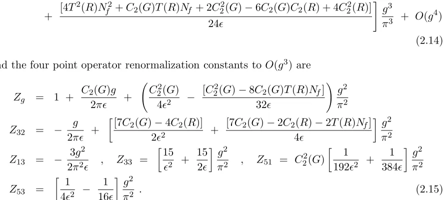
renormalized ones as opposed to those in (2.1) and (2.10) which were assumed to be bare. We find the wave function renormalization constant is

Zψ = 1 −

C2(R)T(R)Nfg2

4π2_ǫ − C2(R)

_C

2(G)T(R)Nf 12ǫ2

+ [4T

2_(R)N2

f +C2(G)T(R)Nf + 2C22(G)−6C2(G)C2(R) + 4C22(R)]

24ǫ

#

g3

π3 + O(g 4₎

(2.14)

and the four point operator renormalization constants to O(g3_{) are}

Zg = 1 +

C2(G)g

2πǫ + C2

2(G)

4ǫ2 −

[C2

2(G)−8C2(G)T(R)Nf] 32ǫ

!

g2

π2

Z32 = −

g

2πǫ +

_[7C

2(G)−4C2(R)]

2ǫ2 +

[7C2(G)−2C2(R)−2T(R)Nf] 4ǫ

_g2

π2

Z13 = −

3g2

2π2_ǫ , Z33 =

₁₅

ǫ2 +

15 2ǫ

_g2

π2 , Z51 = C 2 2(G)

₁

192ǫ2 +

1 384ǫ

_g2

π2

Z53 =

₁

4ǫ2 −

1 16ǫ

_g2

π2 . (2.15)

These values reduce to those quoted in [15] for the caseG=SU(Nc). Although to two loops we have managed to write the generated operators in terms of anti-symmetric or symmetric products of strings of group generators, it is not clear to us whether this should persist to all orders. For example, it may be the case that at a very large loop order the Lie algebra manipulations we used to obtain this Lagrangian do not allow us to reduce the generator products to pure Ta-strings

†_{We use ˜µas the renormalization scale throughout instead of the conventional µsince the latter will}

in that one or more structure functions may remain or three or more traces of generators. A systematic study which goes beyond the symmetric traces of group generators for general Gof [27] would be needed. However, to the order we will be computing the wave function anomalous dimension, (2.13) is all that will be necessary if one considers the topologies of the diagrams which will arise and the operators which can be inserted at various vertices.

We close this section by recalling the relationship of the NATM with other models. As is already well established the abelian Thirring model for Nf = 1 is trivially equivalent to the single flavour Gross Neveu model due to the Fierz identity for the Dirac fermions we are using which is

( ¯ψγµψ)2 = − 2( ¯ψψ)2 . (2.16) Therefore, the renormalization group functions for both models in this limit must agree. How-ever, when one examines the MS renormalization group function in each case it transpires that beyond the leading order there is disagreement which arises because (2.16), which is established using the properties of the strictly two dimensional γ-algebra, is not valid in d-dimensions. Indeed one can use a d-dimensional Fierz lemma, [33, 34], to discover that an infinite set of additional operators emerge on the right side of (2.16) in this case. Therefore, to restore the clear equivalence between the renormalization group functions in both models one needs to make a finite scheme change in the NATM results. Introducing a finite renormalization to ensure a symmetry principle is preserved in the quantum theory is not novel to the NATM. For example, the renormalization of the flavour singlet axial vector current in QCD in MS ceases to preserve the chiral anomaly and one ensures full consistency by a finite renormalization, [35, 36]. Whilst it may appear here that the problem is not related to theγ5 _{issue of the QCD axial anomaly, it}

is in fact implicit in the computation since thed-dimensional object Γµν₍₂₎ would be the projector of the two dimensional γ5. Therefore, as in [15] it will be the case that having established an MS result for the four loop anomalous dimension we will need to determine the constraints on a class of possible scheme changes to preserve the Gross Neveu equivalence. In [17] another equiv-alence was mentioned between the Nf = 3 Gross Neveu model and theNf = 1 SU(4) NATM. Whilst the implications of this were discussed for the three loop NATMβ-function, [15], we will not impose it or discuss it here primarily because it is not clear if a full rigorous proof of the relationship has been established. If one does exist it will be a trivial exercise to determine its consequences for the anomalous dimension. For later use and to illustrate these remarks we now quote the relevant renormalization group functions in MS in both models to the orders they are known. For the Gross Neveu model the anomalous dimension in our notation is [22, 23, 24],

γ(g) = − (2Nf −1)g

2

8π2 +

(2Nf −1)(Nf −1)g3 16π3

− (2Nf −1)(4N

2

f −14Nf + 7)g4

128π4 + O(g

5_{) (2.17)}

and theβ-function is, [21, 23, 24, 37, 38],

β(g) = − (Nf −1)g

2

π +

(Nf −1)g3 2π2 +

(2Nf−7)(Nf −1)g4

16π3 + O(g

5_{) (2.18)}

where we note that the Gross Neveu Lagrangian is, [21],

LGN = iψ¯i∂/ψi + g 2

¯

ψiψi2 . (2.19)

For the NATM the anomalous dimension is, [14, 15, 18, 19],

γ(g) = − C2(R)T(R)Nfg

2

+ h2C2(G)C2(R)−C22(G)−2C2(G)T(R)Nf −8T2(R)Nf2

iC₂(R)g3

16π3 + O(g 4₎

(2.20)

and theβ-function is, [1, 14, 17, 15],

β(g) = C2(G)g

2

2π +

T(R)NfC2(G)g3

2π2

+C2(G)

₅

8T

2_(R)N2

f + 39 16C

2 2(R) −

67

32C2(R)C2(G) + 31 64C

2 2(G)

_g4

π3 + O(g 5_{) .}

(2.21)

We also note that several all orders results are available in the Thirring model, though it is not clear if they are in an MS scheme. In the abelian case, [39],

γ(g) = − Nfg

2

2π2₁₋ Nfg

π

, β(g) = 0. (2.22)

For the NATM, Kutasov has written down an expression for β(g) which has a similar form to (2.22), [40]. In the current notation of this paper it is

β(g) = C2(G)g

2

2π1−T(R)Nfg

2π

2 . (2.23)

This expression was established through a connection the two dimensional theory has with string and conformal field theory but was in fact only valid whenNf is large. More recently, however, by using current algebra Ward identities this result has been argued to be exact at all orders in a particular scheme, [41]. This is an important point since it only contains the elementary Casimirs of G and not the higher order ones which we are concerned with here. Whilst (2.23) would put additional constraints on potential scheme changes needed for theβ-function we will not need to consider these here as they will not play a role in the analysis of the anomalous dimension.

3

Four loop calculations.

We are now in a position to carry out the four loop renormalization of the wave function in (2.1) using the d-dimensional evanescent Lagrangian of (2.13). First, we redo the three loop calculation of [15, 17, 18, 19] but for the case of a general Lie group. Unlike [15] we will use the massless propagator

ip/

p2 (3.1)

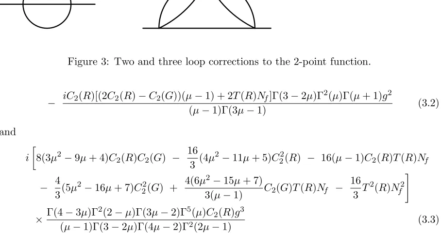
spurious infrared infinities ought not to arise at the order we are working to since, for instance, neither external momentum is nullified. Therefore, in all our calculations we use (3.1) without an infrared mass regularization and this allows us in fact to calculate all the necessary integrals exactly to four loops or at least to the finite part in ǫ. This latter property is important since we will be considering scheme changes later and it is necessary to have the renormalized Green’s function in order to extract the renormalization group function in various schemes. Further, by choosing a massless propagator the Feynman diagrams with tadpoles‡ are absent since by Lorentz invariance the tadpole subintegral is zero. Therefore to three loops the only two basic topologies which are relevant for the wave function renormalization are those given in figure 3. They can be evaluated exactly as a function of d= 2µand we find that they are respectively

Figure 3: Two and three loop corrections to the 2-point function.

− iC2(R)[(2C2(R)−C2(G))(µ−1) + 2T(R)Nf]Γ(3−2µ)Γ

2_{(µ)Γ(µ+ 1)g}2

(µ−1)Γ(3µ−1) (3.2) and

i

8(3µ2−9µ+ 4)C2(R)C2(G) −

16 3 (4µ

2_{−11µ+ 5)C}2

2(R) − 16(µ−1)C2(R)T(R)Nf

− 4

3(5µ

2_{−16µ+ 7)C}2 2(G) +

4(6µ2−15µ+ 7)

3(µ−1) C2(G)T(R)Nf − 16

3 T

2_(R)N2

f #

× Γ(4−3µ)Γ

2_{(2−µ)Γ(3µ−2)Γ}5_(µ)C 2(R)g3

(µ−1)Γ(3−2µ)Γ(4µ−2)Γ2_(2µ−1) (3.3)

where we have omitted here and in later values of Feynman graphs, the overall power of the momentum and renormalization scale ˜µ, which can be restored on dimensional grounds,p/, where

p is the external momentum, and factors of (4π)d/2. Also the coupling constant g which will appear in the values is bare. However, for the full three loop anomalous dimension to be deduced correctly we need to take account of the contribution from the generated evanescent operator

O32 which is represented by the Feynman diagrams of figure 4. In these graphs the γ-algebra

now involves the Γ₍₃₎-matrix sandwiched between ordinary γ-matrices. To handle this in the

Figure 4: Single evanescent operator contributions to the 3 loop 2-point function.

computation we decompose Γ(3) into its six terms, multiply the γ-string by p/ and take the

trace as well as dividing by the normalization of 2p2. To cope with the algebra generated and the mundane massless integration in this and other graphs we have made use of the symbolic

manipulation programme Form_{, [25]. Moreover, to ensure that the integration routines are}

properly constructed we have repeated the full four loop anomalous dimension calculation of [22] in the SU(N) Gross Neveu model and reproduced the result of [22]. Having verified the programmes reproduce the correct results for this model it is then elementary to re-run them where the input Lagrangian is replaced by the NATM. Whilst evanescent operators will not be present in the four loop Gross Neveu calculation the integration routines were still valid for the NATM since we evaluated systematically all the basic scalar integrals which could arise in any of the topologies. Although the decomposition of Γ₍₃₎ for the graph of figure 3 was relatively efficient, for higher order Γ(n)’s or for diagrams with more than one evanescent operator insertion,

it was much more appropriate to make use of the general properties of the Γ(n)’s in these cases.

For example, the lemma, [17, 18, 31],

Γµ1...µn

(n) Γ

ν1...νm

(m) Γ (n)

µ1...µn = f(n, m)Γ

ν1...νm

(m) (3.4)

where

f(n, m) = (−1)nm(−1)n(n−1)/2 ∂ n

∂un h

(1 +u)d−m(1−u)mi

u=0

(3.5)

led to the other graphs being determined relatively quickly. Hence, we record the value of the graphs of figure 4 are

iC2(R)[3C2(G)−4C2(R)][C2(G)−2C2(R)](2µ−1)(µ−3)µΓ(3−2µ)Γ3(µ)g3

Γ(3µ−1) . (3.6)

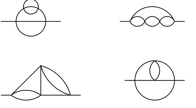
We now turn to the details of the four loop calculation. The basic topologies are given in figure 5 and fall into two classes. The upper two Feynman diagrams correspond to elementary

Figure 5: Four loop corrections to the 2-point function.

massless chain integrals and can therefore be computed straightforwardly. We find their d -dimensional values are respectively

3iC₂2(R)

2C2(G)C2(R) − 2C22(R) −

4C2(R)T(R)Nf (µ−1) −

1 2C

2 2(G)

+ 2C2(G)T(R)Nf (µ−1) −

2T2_(R)N2

f (µ−1)2

#

µ2_{Γ(5−4µ)Γ}5_(µ)g4

and

i

"

12(32µ4_−213µ3_{+ 581µ}2_{−514µ+ 144)C}

2(G)C23(R)

(µ−1)

− 4(56µ

4_−301µ3_{+ 701µ}2_{−586µ+ 160)C}4 2(R)

(µ−1)

− 96(3µ−2)(µ−1)C₂3(R)T(R)Nf + 32(3µ−2)C2(G)C2(R)T2(R)Nf2

− (232µ

4_−1903µ3_{+ 5791µ}2_{−5294µ+ 1504)C}2

2(G)C22(R)

(µ−1)

+ 96(3µ−2)(µ−1)C2(G)C22(R)T(R)Nf −

16(3µ−2)C2(R)T3(R)Nf3 (µ−1)

+ (296µ

4_−2903µ3_{+ 9479µ}2_{−8830µ+ 2528)C}3

2(G)C2(R)

6(µ−1)

− (432µ

5_−2004µ4_{+ 3863µ}3_−3693µ2_{+ 1734µ−320)C}2

2(G)C2(R)T(R)Nf 6(µ−1)3

− 4(8µ

4_−125µ3_{+ 461µ}2_{−442µ+ 128)d}abcd A dabcdF (µ−1)N_fund

− 2(12µ

4_{+ 119µ}3_−237µ2_{+ 150µ−32)d}abcd

F dabcdF Nf (µ−1)3_N

fund

− 64(3µ−2)C₂2(R)T2(R)N_f2i Γ(5−4µ)Γ(4µ−3)Γ

3_(2−µ)Γ7_(µ)g4

(2µ−1)2_{Γ(5µ−3)Γ(4−3µ)Γ}3_(2µ−1) . (3.8)

Although these are elementary to derive we draw attention to the group theory structure of each result. The former since it has a propagator correction involves the usual products of Casimirs which arise at lower order. By contrast the embedded chain diagram involves the two new Casimirs constructed from the tensors dF and dA. It is instructive to consider how these arise. Clearly the term dabcd_F dabcd_F arises from two strings of group generators where one of the

TafromTa⊗Tatensor structure is located in one string with the other in the second string. On the other hand the second new combination arises from manipulating particular strings of eight generators. They are all related to TrTaTbTcTdTaTbTcTd. Using the Lie algebra, (2.2), it is elementary to deduce

TrTaTbTcTdTaTbTcTd = " ₃

Y

r=0

C2(R)−

r

2C2(G)

− 1

8C

3

2(G)C2(R)

#

N_fund

+fapqfbqrfcrsfdspTrTaTbTcTd . (3.9)

Examining the last term reveals that the combination of structure constants is equivalent to TrAaAbAcAd whereAa is the adjoint representation of the generators and hence this string can be related to the dabcd

F dabcdA term. One can also consider the group theory of this diagram from the point of view of the connection with QCD. In (2.1) it is possible to write the four point interaction in terms of a spin-1 auxiliary field which in d-dimensions is related to the gluon of QCD. In such a reformulation the second diagram of figure 5 would correspond to the first graph of figure 6 where the spring line is the auxiliary field. Clearly one can identify the dabcd_F dabcd_F structure that is contained in the topology. However, it is not evident how the

Figure 6: Four loop self-energy corrections in QCD containing dabcd_F dabcd_F and dabcd_F dabcd_A respec-tively.

that there is a potential inconsistency in our evaluation. However, as will become apparent later this issue will be satisfactorily resolved. For the remaining two diagrams of figure 5 we expect

dabcd_F dabcd_F anddabcd_F dabcd_A terms to be present after considering the routing of the group generator strings in the graphs.

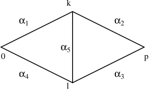
The main point concerning these two diagrams is that their evaluation rests in the fact that unlike the previous graphs discussed so far they do not reduce to simple chain integrals. Instead upon taking the spinor trace and evaluating two elementary loop integrations one is left with a set of two loop integrals which need to be evaluated. These have the general form of figure 7 where we use coordinate space representation where the internal momenta k and l

α4 α1

α5

α3 α2

0

l k

p

Figure 7: General two loop self energy topology whose value is denoted by hα1, α2, α3, α4, α5i.

are integrated over. The αi beside a line denotes the power to which that scalar propagator is raised to. The graphs either involve tensor numerators or are purely scalar. For the former case given the large symmetry of the diagram one can always rewrite such numerator scalar products in terms of denominator factors which then reduce the exponent of that line by unity. After this procedure one is left with diagrams which are either chains or purely scalar two loop graphs. For each of the graphs of figure 5 this remaining topology has the same pattern of exponents. For the third graph we find {αi} = {1, α,1, β,1} and for the final graph {αi} =

{1,1,1,1, α} whereα and β here are functions of d and therefore non-integer whend= 2 −ǫ. By integration by parts rules and recurrence relations based on the uniqueness rule of [42, 43] one can reduce this set of graphs either to chain diagrams or to two respective d-dimensional basis scalar integrals given byh1,1−µ,1,1−µ,1iand h1,1,1,1,1−µiwhere we have again set

chain integrals. In [26] the Gram method was applied to a particular choice of the{αi}. In the appendix we briefly recall the arguments and record the general expression for the relation. In, for example, the application of the rule of (A.4) to the set of the form h1,1,1,1, αi the ninth and tenth terms of (A.4) correspond to the same original topology. The actual combination of exponents can be restored by the recurrence relations of [44]. Having related these two basic integrals to ones in (4−ǫ)-dimensions, the ǫ expansion of the higher dimensional integral is determined from the results of [45, 46]. Whilst theǫ-expansion is known for the general integral to O(ǫ4_{), [45], only the first term is relevant to our two dimensional calculation as the factors of}

(µ−1) ensure the leading term appears in the finite part. It might be thought that the group theory and symmetry arguments used in [45, 46] to deduce the ǫ-expansion of the problematic two dimensional integrals could be used directly on them. However, these arguments seem to rely in part on the fact that in four dimensions the diagram is finite with respect to ǫ and the leading term of the expansion is independent of {αi} for {αi} of O(ǫ) from unity. In two dimensions the diagram is singular inǫand as the residue of the pole depends on the parameters it does not appear possible for the group theory arguments of [45, 46] to proceed. Given these remarks we record the value of the third graph of figure 5 is

ih8(49µ4 −336µ3+ 794µ2−832µ+ 283)C2(G)C23(R)

− 8(27µ4−174µ3+ 392µ2−394µ+ 131)C₂4(R)

− 8(µ−1)(18µ2−59µ+ 32)C₂3(R)T(R)Nf − 4(6µ2−15µ+ 8)C22(R)T2(R)Nf2

− 4(59µ4−430µ3+ 1072µ2−1178µ+ 411)C₂2(G)C₂2(R) + 4(µ−1)(42µ2−161µ+ 88)C2(G)C22(R)T(R)Nf + 4

3(36µ

4_−281µ3_{+ 747µ}2_{−867µ+ 311)C}3

2(G)C2(R)

− (576µ

4_−3604µ3_{+ 6853µ}2_{−5159µ+ 1346)C}2

2(G)C2(R)T(R)Nf 12(µ−1)

+ 2(6µ2−29µ+ 16)C2(G)C2(R)T2(R)Nf2

− 8(3µ

4_−38µ3_{+ 144µ}2_{−210µ+ 83)d}abcd A dabcdF

N_fund

− 2(4µ

3_−37µ2_{+ 23µ−2)d}abcd

F dabcdF Nf (µ−1)N_fund

!

Γ2(3−2µ)Γ6(µ)

(µ−1)2_{(2µ−1)(5µ−4)Γ}2_(3µ−2)

+ 384(77µ5−605µ4+ 1743µ3−2395µ2+ 1498µ−346)(µ−1)C2(G)C23(R)

− 384(41µ5−304µ4+ 842µ3−1124µ2 + 691µ−158)(µ−1)C₂4(R)

− 768(12µ3−47µ2+ 49µ−16)(µ−1)2C₂3(R)T(R)Nf

− 192(97µ5−804µ4+ 2414µ3−3424µ2+ 2183µ−510)(µ−1)C₂2(G)C₂2(R) + 1536(7µ3−32µ2+ 34µ−11)(µ−1)2C2(G)C22(R)T(R)Nf

− 1536(µ−1)4C₂2(R)T2(R)N_f2

+ 32(126µ5−1103µ4+ 3467µ3−5093µ2+ 3315µ−784)(µ−1)C₂3(G)C2(R)

− 8(384µ5−2713µ4+ 6378µ3−6806µ2+ 3431µ−670)C₂2(G)C2(R)T(R)Nf + 192(4µ3−23µ2+ 25µ−8)(µ−1)C2(G)C2(R)T2(R)Nf2

− 384(9µ5−100µ4+ 382µ3−640µ2+ 447µ−110)(µ−1)d abcd A dabcdF

N_fund

− 192(µ4−18µ3+ 14µ2+µ−2)d

abcd

F dabcdF Nf

N_fund

!

Γ2_(2−µ)Γ4_(µ)

× h1,2−µ,1,2−µ,1i

_µ+1

+ 4(19µ

4_−126µ3_{+ 294µ}2_{−304µ+ 105)C}4 2(R)

(µ−1) + 16(3µ

2 _{−10µ+ 6)C}3

2(R)T(R)Nf

− 4(35µ

4_−247µ3_{+ 603µ}2_{−647µ+ 228)C}

2(G)C23(R)

(µ−1) + 2(43µ

4_−322µ3_{+ 826µ}2_{−924µ+ 333)C}2

2(G)C22(R)

(µ−1)

− 4(14µ2−55µ+ 33)C2(G)C22(R)T(R)Nf + 4(2µ−3)C22(R)T2(R)Nf2

− (54µ

4_−431µ3_{+ 1171µ}2_{−1373µ+ 507)C}3

2(G)C2(R)

3(µ−1) + (192µ

4_−1225µ3_{+ 2387µ}2_{−1854µ+ 504)C}2

2(G)C2(R)T(R)Nf 12(µ−1)2

− 4(µ

2_{−5µ+ 3)C}

2(G)C2(R)T2(R)Nf2 (µ−1)

+ 4(3µ

4_−34µ3_{+ 122µ}2_{−172µ+ 69)d}abcd A dabcdF (µ−1)N_fund

+ 2µ(µ

2_{−11µ+ 6)d}abcd

F dabcdF Nf (µ−1)2_N

fund

!

Γ(5−4µ)Γ5_(µ)

(µ−1)(2µ−1)Γ(5µ−3) #

g4 . (3.10)

The term h1,2−µ,1,2−µ,1i

µ+1corresponds to the higher dimensional integral derived in the

Gram determinant method where the restriction denotes a 2(µ+ 1)-dimensional measure. Space prevents us from recording the exact value of the remaining graph since it is of a comparable size to (3.10) though we note it has a similar form.

To complete the full four loop calculation the contributions from the evanescent operators need to be included. One can divide these into the diagrams which involve the operator generated at one loop in the four point function and those arising from the two loop ones. For the latter, the relevant topologies are those of figure 2. We record the respective values of the graphs and include the appropriate renormalization constant to aid identification. They are, in addition to (3.6) which involves Z32,

iZ13

9C2(G)C23(R) − 4C24(R) −

20 3 C

2

2(G)C22(R) +

5 3C

3

2(G)C2(R)

− 2d

abcd A dabcdF

N_fund −

4dabcd_F dabcd_F Nf (µ−1)N_fund

#

µΓ(3−2µ)Γ3(µ)g2

Γ(3µ−1) (3.11)

4iZ31C2(R)[2C2(R)−C2(G)]

µ(2µ−1)(µ−3)Γ(3−2µ)Γ3(µ)g2

Γ(3µ−1) (3.12)

iZ33

₂

3C2(G)C

3 2(R) −

2 3C

2

2(G)C22(R) +

1 9C

3

2(G)C2(R)

+ 4d abcd A dabcdF 3N_fund

#

µ(2µ−1)(µ−3)Γ(3−2µ)Γ3(µ)g2

Γ(3µ−1) (3.13)

8iZ51C2(R)[2C2(R)−C2(G)]µ(2µ−1)(µ−2)(µ−5)

Γ(4−2µ)Γ3(µ)g2

and

iZ53

18C2(G)C23(R) − 8C24(R) −

40 3 C

2

2(G)C22(R) +

10 3 C

3

2(G)C2(R)

− 4d

abcd A dabcdF

N_fund

#

µ(2µ−1)(µ−5)Γ(5−2µ)Γ3(µ)g2

Γ(3µ−1) . (3.15)

These explicit values illustrate that even though they are two loop topologies some do contain the new Casimir structures that appear at four loops. This is because unlike the original interaction these operator insertions have more than one pair of group generators. Hence the strings of

Figure 8: Double evanescent operator correction to the 4 loop 2-point function.

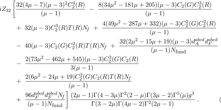
group generators can contain one set of eight Ta’s. The remaining set of contributions come from the insertion of O32 in the topologies illustrated in figures 8 and 9. For the three loop

Figure 9: Single evanescent operator correction to the 4 loop 2-point function.

topologies their values are

iZ32

"

32(4µ−7)(µ−3)2C₂4(R) (µ−1) −

8(34µ2−181µ+ 205)(µ−3)C2(G)C23(R)

(µ−1)

+ 32(µ−3)C₂3(R)T(R)Nf +

4(49µ2−287µ+ 332)(µ−3)C₂2(G)C₂2(R) (µ−1)

− 40(µ−3)C2(G)C22(R)T(R)Nf +

32(2µ2−15µ+ 19)(µ−3)dabcd_A dabcd_F

(µ−1)N_fund

− 2(73µ

2_{−462µ+ 545)(µ−3)C}3

2(G)C2(R)

3(µ−1) + 2(6µ

2_{−24µ+ 19)C}2

2(G)C2(R)T(R)Nf (µ−1)

+ 96d abcd

F dabcdF Nf (µ−1)N_fund

#

(2µ−1)Γ(4−3µ)Γ2(2−µ)Γ(3µ−2)Γ5(µ)g3

Γ(3−2µ)Γ(4µ−2)Γ2_(2µ−1) . (3.16)

Whilst the diagram with a double operator insertion has the value

iZ₃₂2 h20(2µ2−15µ+ 19)(µ−3)C2(G)C23(R) − 8(2µ2−15µ+ 19)(µ−3)C24(R)

− 33(2µ

2_{−15µ+ 19)(µ−3)C}2

2(G)C22(R)

2 −

+ 55(2µ

2_{−15µ+ 19)(µ−3)C}3

2(G)C2(R)

12 −

8(2µ2−15µ+ 19)(µ−3)dabcd_A dabcd_F N_fund

− 24d

abcd

F dabcdF Nf

N_fund

#

µ(2µ−1)Γ(3−2µ)Γ3(µ)g2

Γ(3µ−1) . (3.17)

This diagram contributes when one considers the powers of the coupling constant which are present. This completes the evaluation of all the diagrams relevant for the renormalization of the two point function at four loops.

4

Four loop anomalous dimension.

Having determined all the contributions to the two point function including those from evanes-cent operator insertions it is a relatively straightforward task to determine the four loop correc-tion to the wave funccorrec-tion renormalizacorrec-tion. We find

Z_ψMS = 1 − C2(R)T(R)Nfg

2

4π2_ǫ − C2(R)

_C

2(G)T(R)Nf 12ǫ2

+ [4T2(R)N_f2+C2(G)T(R)Nf + 2C22(G)−6C2(R)C2(G) + 4C22(R)]

1 24ǫ

_g3

π3

−

"

T(R)NfC2(R)C22(G)

32ǫ3 + 192

dabcd_A dabcd_F N_fund −48

NfdabcdF dabcdF

N_fund −96C

3

2(G)C2(R)

+ 352C₂2(G)C₂2(R) + 3C₂2(G)C2(R)T(R)Nf −448C2(G)C23(R)

+ 32C2(G)C2(R)T2(R)Nf2+ 192C24(R)−8C22(R)T2(R)Nf2

₁

256ǫ2

+ 772C₂3(G)C2(R)−1536

dabcd_A dabcd_F N_fund −624

dabcd_F dabcd_F Nf

N_fund

−2808C₂2(G)C₂2(R) + 299C₂2(G)C2(R)T(R)Nf + 3552C2(G)C23(R)

−864C2(G)C22(R)T(R)Nf −1536C24(R) + 576C23(R)T(R)Nf + 192C2(R)T3(R)Nf3

₁

1536ǫ

_g4

π4 + O(g

5_{) . (4.1)}

Ordinarily one does not quote this value but merely gives the corresponding anomalous dimen-sion. We have done so here to illustrate an important feature of renormalizing a model with evanescent operators. For ordinary (single coupling) theories where this is not an issue the poles of the MS renormalization constants are related in a particular way. For example, the residues of the non-simple poles are determined by the simple pole residues at lower orders, [47]. How-ever, examining (4.1) one can see that this is not the case since at four loops the new Casimir contributions occur in the residue of the double pole inǫ. Usually this would indicate an error in the renormalization since these new Casimirs cannot arise before four loops and so they should only appear in the simple pole inǫ. In this instance, however, the choice (4.1) correctly renders the two point function finite but the anomalous dimension derived from it corresponds to the na¨ıve renormalization group function and not the true one in relation to the discussion of section 2. To obtain the true anomalous dimension there are two possible procedures to follow. One is to extend the projection technique developed in [20, 17] and applied to the SU(Nc) NATM

true renormalization group function. The alternative approach which produces the equivalent result is to ensure that the finite renormalized two point function in two dimensions satisfies the renormalization group equation

˜

µ∂

∂µ˜ + β(g)

∂ ∂g +

n

2γ(g)

Γ(n)(p,µ, g˜ ) = 0 (4.2)

where Γ(n)_{(p,µ, g˜ ) is the renormalized n-point Green’s function. To ensure this condition can}

be used one must be careful in retaining the finite parts of all the integrals in the construction of the Green’s function before renormalization. This is the reason why we have been careful to compute the integrals exactly in most cases and to sufficient powers in ǫin the other cases and means we will follow the latter course here. After renormalization the two point function is

Γ(2)(p,µ, g˜ ) = "

1 + C2(R) 4T(R)Nf +C2(G)−2C2(R)−4T(R)Nfln

p2

ˆ

µ2

!!

g2

16π2

+ 12T(R)Nf(C2(G)−4T(R)Nf) ln

p2

ˆ

µ2

!

−12C2(G)T(R)Nfln2

p2

ˆ

µ2

!

− 19C₂2(G) + 66C2(G)C2(R) + 16C2(G)T(R)Nf − 56C22(R)

− 48C2(R)T(R)Nf + 64T2(R)Nf2

C₂(R)g3 192π3

+ 2112d abcd A dabcdF

N_fund − 48C

2

2(G)C2(R)T(R)Nfln3

p2

ˆ

µ2

!

+ 243C₂2(G)−20C2(G)T(R)Nf + 4C2(R)T(R)Nf

×C2(R)T(R)Nfln2

p2

ˆ

µ2

!

+ 96C₂3(R)T(R)Nf − 44C22(G)C2(R)T(R)Nf − 192C22(R)T2(R)Nf2

− 240C2(G)C22(R)T(R)Nf + 1152C2(G)C2(R)T2(R)Nf2

− 768C2(R)T3(R)Nf3 + 2496

dabcd_F dabcd_F Nf

N_fund ! ln p 2 ˆ µ2 !

− 1147C₂3(G)C2(R) + 4452C22(G)C22(R) + 1152C2(R)T3(R)Nf3

− 870C₂2(G)C2(R)T(R)Nf − 6096C2(G)C23(R)

+ 3408C2(G)C22(R)T(R)Nf − 624C2(G)C2(R)T2(R)Nf2 + 2856C₂4(R) − 2688C₂3(R)T(R)Nf − 1056C22(R)T2(R)Nf2

+ (576ζ(3)−3312)d abcd

F dabcdF Nf

N_fund

!

g4

3072π4

#

ip/ + O(g5) (4.3)

where ˜µ2 = 4πe−γµˆ2 and γ is the Euler-Mascheroni constant. Hence, using the three loop MS

β-function of [15] we find that for a general colour group the MS result is

γMS(g) = −C2(R)T(R)Nf

g2

2π2

+ h2C2(G)C2(R)−C22(G)−2C2(G)T(R)Nf −8T2(R)Nf2

iC₂(R)g3 16π3

+ "

624Nfd abcd F dabcdF

N_fund + 57C

3

2(G)C2(R)−198C22(G)C22(R)

−192C2(R)T3(R)Nf3 i g4

384π4 + O(g

5_{). (4.4)}

As a check on this value we have in fact applied the projection formalism to the case when

G=SU(Nc) and verified that both are in agreement. One interesting feature of the expression (4.4) is that the new Casimir dabcd

A dabcdF has cancelled in the final expression leaving only a term involving dabcd_F dabcd_F . This cancellation appears to be consistent with our earlier discussion on the nature of the graphs in the two point function when regarded from a QCD point of view and also reflects the contribution from the relevant evanescent operators. Though we do not regard this observation as a hard check on the final result. More importantly from the point of view of our original motivation a new Casimir does appear in the (MS) anomalous dimension of the fermion.

Whilst we have produced the MS anomalous dimension at four loops there remains one final task to perform which has been discussed in related work. This rests in the nature of the dimen-sional regularization. In two dimensions one has various equivalences between certain models such as the abelian Thirring model being the same as the Gross Neveu model forNf = 1. This is established through an elementary two dimensional Fierz transformation. Ind-dimensions, how-ever, such relations cannot be preserved. In the first instance, the Fierz transformation becomes infinite dimensional as one has to decomposeI⊗I into the full basis of tensor products of Γ_(n), [33, 34]. Secondly, the relation that one can establish depends on the evanescent operators which are generated in the four point interaction but not in a way which the direct relationship can be determined. Therefore the situation is such that in renormalizing the NATM, the resulting MS renormalization group functions do not preserve the specific equivalences. In other words taking the abelian limit of (4.4) does not recover the four loop result of [22] for theNf = 1 Gross Neveu model. To ensure that this property is preserved in the renormalization having been broken by the regularization, we need to make a finite scheme change. Such changes were considered inall previous work in this area, [16, 17, 18, 19], and we proceed along similar lines to [15] here.

As the choice of possible scheme changes is infinite we restrict our study to the class intro-duced in [15]. There the scheme was changed from MS to one where the finite part was also absorbed into the renormalization constants. In order to examine the equivalences the finite part is parametrised and constraints placed on the parameters by ensuring agreement of the renormalization group functions in the various limits. Whilst this may introduce a large degree of redundancy it allows for choices in future applications of the results. Here as we are dealing with a general group G we use the usual Casimirs as the basis for the parametrization of the finite part. In particular we choose the finite part of Zψ to be

C2(R) [w21C2(R) +w22C2(G) +w23T(R)Nf]

g2 π2

+C2(R)

h

w31C22(R) +w32C22(G) +w33T2(R)Nf2+w34C2(G)C2(R)

+w35C2(R)T(R)Nf +w36C2(G)T(R)Nf _g3

π3 + O(g

4_{) (4.5)}

anomalous dimension is

γgen(¯g) = −C2(R)T(R)Nf ¯

g2

2π2

−C2(R)

h

b11+12

T2(R)N_f2+b13C2(R)T(R)Nf + w23+b12+18

C2(G)T(R)Nf

+ w21−18

C2(G)C2(R) + w22+161

C₂2(G)i g¯

3

π3

− h1

2

b2₁₁+ 3b11+ 2b21+ 1

C2(R)T3(R)Nf3

+ b23−2w23+32b13+b11b13

C₂2(R)T2(R)N_f2

+ b11b12+ 38b11+ 3

2b12+b22+w23+ 3 2w33

C2(G)C2(R)T2(R)Nf2

+b26−2w21+12b

2 13

C₂3(R)T(R)Nf

− 2w22−32w35+

3

8−w21−b25− 3

8b13−b12b13+ 3 8b11

C2(G)C22(R)T(R)Nf

+3 2w36+

83

576 +w22+b24+ 1 2b

2 12+

3 8b12+

3 16b11

C₂2(G)C2(R)T(R)Nf

+ 3 2w31−

7 16−

3 8b13

C2(G)C23(R) +

3 2w34+

33 64 +

3 16b13−

3 8b12

C₂2(G)C₂2(R)

+ 3 2w32−

19 128+

3 16b12

C₂3(G)C2(R)−

13dabcd_F dabcd_F Nf 8N_fund

# ¯

g4

π4 + O(¯g

5_{) (4.6)}

where ¯g denotes the coupling constant of the new scheme and we have taken the finite part of the renormalization constant Z_ψ2Zg to be

[b11T(R)Nf +b12C2(G) +b13C2(R)]

g π

+ hb21T2(R)Nf2+b22T(R)NfC2(G) +b23C2(R)T(R)Nf

+b24C22(G) +b25C2(R)C2(G) +b26C22(R)

ig2

π2 + O(g

3_{) . (4.7)}

Whilst we have discussed the constraints on the three loop parameters in [15] we will redo that calculation here. This is partly to do with the fact that there were restrictions from two equivalences and for reasons already discussed we will only consider the one relating the abelian Thirring model and the Gross Neveu model. For this we recall that the abelian limit of the Casimirs is

C2(R) → 1 , C2(G) → 0 , T(R) → 1 , dabcdF dabcdF → 1 . (4.8) Therefore, we find the constraints

b11 + b13 = −

1 2

b21 + b23 + b26 − 2w21 − 2w23 =

11

8 (4.9)

Whilst these do not restrict the values of the parameters substantially any (numerical) choice must satisfy these equations for the two dimensional symmetry broken in d-dimensions to be established. The first equation of (4.9) agrees with that of [15] when the parameters are converted to the case of G=SU(Nc).

5

Discussion.

in QCD. Whilst one of the two potential new Casimirs is absent in (4.4) the one involving the fundamental representation remains. Therefore if the connection between the WZWN model and the NATM critical exponents is valid then the problem of how such a term cancels in the final critical exponent when approached from the renormalization group equation point of view is still open. One possibility is that of choosing a renormalization scheme in such a way that this new term is absent from (4.4). Although this would appear to resolve the issue it has implications for the other renormalization group functions as this scheme choice impinges on how one renormalizes their associated Green’s function. In particular this will impact upon the

β-function and it is possible they will be transformed into it. Even if this were not the case, the computation ofβ(g) itself at four loops in the NATM will produce these new Casimirs as well, which can be seen from examining the group theory of the Feynman diagrams of the fermion four point function. This would appear to contradict the recent exact β-function of [41]. However, in that case it seems that the use of conformal symmetry has somehow excluded the higher order Casimirs. A similar feature occurs in four dimensional gauge theories at four loops. If one examines the four loop MSβ-function of QCD, [12], for an arbitrary colour group the terms involving dF and dA will vanish in certain cases. For instance, when the quark is in the adjoint representation andNf = 12 then the resultingβ-function contains no higher order Casimirs. This is, of course, the result of the theory possessing a new symmetry which isN = 1 supersymmetry. Thus, in the NATM it may be that a similar mechanism such as the two dimensional conformal symmetry used in the construction of [41] is responsible and powerful enough to exclude the

dabcd

F dabcdF term in the NATM β-function to all orders in a particular renormalization scheme. Though it is not clear in this approach what form the all orders fermion anomalous dimension would take. Alternatively from the critical exponent point of view since β(g) will contain information on the non-trivial fixed point, gc, at which the renormalization group functions are evaluated at to obtain the critical exponents, to examine the mechanics of the Casimir cancellation further would require the explicit form of the four loop NATMβ-function in order to carry out a test of this point of view at this order of approximation. The complexity of such a calculation is on a footing equal to the renormalization of the two point function atfiveloops. Moreover, the four loop β-function of the usual simple Gross Neveu model, which would serve as a preliminary to a similar calculation in the NATM, has yet to be performed. Therefore, to understand this further would require a substantial amount of new calculations beyond those performed here.

Acknowledgements. This work was carried out with the support of PPARC _{through a}

Postgraduate Studentship (DBA) and an Advanced Fellowship (JAG). The calculations were performed with the help of the computer algebra and symbolic manipulation programmesForm_,

[25], andReduce_{, [48].}

A

Gram determinant.

In this appendix we briefly recall the application of the Gram determinant method of [26] to relate a two loop self energy integral in (d+2)-dimensions to a set ofd-dimensional integrals. The method relies on several properties. First, thed-dimensional measure of a (massless) Feynman integral can be related through

dd+2x = 2πx

2

d d

Next the Gram determinant of three Lorentz vectors, x,y and z, is defined by

Gr(x, y, z) = det 

 

x2 _{xy xz}

yx y2 yz zx zy z2





 (A.2)

and through considering the Lorentz invariance of each integration, one can show that, [22],

Z

ddx

Z

ddy

Z

ddz Gr(x, y, z)F(b1x2+b2y2+b3z2)

= d(d−1)(d−2) (2π)3

Z

dd+2x

Z

dd+2y

Z

dd+2z F(b1x2+b2y2+b3z2) (A.3)

where F(x) is a general function. In our case it represents the Feynman parametized two loop self energy graph of figure 7 when converted into a vacuum diagram. For this topology one can always write the integral as a linear combination of the three Lorentz invariants x2,y2 and

z2 where y and z represent the internal k and l momentum integrations and x corresponds to an integration over the endpoint to produce the three loop vacuum bubble. Since the Gram determinant is invariant under the change of variables used to produce the form of the argument ofF(x) in (A.3) one can undo this transformation and replaceF(x) by the two loop topology of figure 7. As the finalx-integration is then the same for both sides one can relate thevaluesof the integrals on both sides quite straightforwardly. Indeed, expanding out the Gram determinant and expressing all the scalar products in terms of factors which appear in the denominator, one obtains the general result which is implicit in [22]. We have

hα1, α2, α3, α4, α5i

_µ+1

=

[−1,0,0,0,−1] − [−1,−1,0,0,0] + [−1,0,−1,0,0] + [0,0,0,−1,−1] + [0,−1,0,−1,0] − [0,0,−1,−1,0] + [0,−1,0,0,−1] + [0,0,−1,0,−1] − [0,0,0,0,−2]

− [0,0,0,0,−1]− − [−1,0,0,−1,−1]+ + [−1,−1,0,−1,0]+

+ [−1,0,−1,−1,0]+ + [−1,0,−1,0,−1]+ + [−1,−1,−1,0,0]+

− [−1,0,−2,0,0]+ − [−2,0,−1,0,0]+ + [0,−1,0,−1,−1]+

+ [0,−1,−1,−1,0]+ − [0,−2,0,−1,0]+ − [0,−1,0,−2,0]+

− [0,−1,−1,0,−1]+

₁

2(µ−1)(2µ−1) (A.4) where

[n1, n2, n3, n5, n5]n6 = hα1+n1, α2+n2, α3+n3, α4+n4, α5+n5i

1

(x2₎n6 (A.5)

References.

[1] R. Dashen & Y. Frishman, Phys. Lett. B46 (1973), 439; Phys. Rev. D11(1975), 2781.

[2] E. Witten, Commun. Math. Phys. 92(1984), 455.

[3] V.G. Knizhnik & A.B. Zamolodchikov, Nucl. Phys. B257 (1984), 83.

[4] M. Bos, Phys. Lett. B189 (1987), 435; Ann. Phys.181 (1988), 177.

[5] Z-M. Xi, Phys. Lett. B214 (1988), 204; Nucl. Phys.B314 (1989), 112.

[6] A. Hasenfratz & P. Hasenfratz, Phys. Lett.B297 (1992), 166.

[7] J.A. Gracey, Phys. Lett.B373 (1996), 178.

[8] J.A. Gracey, Phys. Lett.B322(1994), 141; J.F. Bennett & J.A. Gracey, Nucl. Phys.B517

(1998), 241.

[9] M. Ciuchini, S.´E. Derkachov, J.A. Gracey & A.N. Manashov, Nucl. Phys.B579 (2000), 56.

[10] K.G. Chetyrkin, Phys. Lett.B404 (1997), 161.

[11] J.A.M. Vermaseren, S.A. Larin & T. van Ritbergen, Phys. Lett.B405 (1997), 327.

[12] T. van Ritbergen, J.A.M. Vermaseren & S.A. Larin, Phys. Lett.B400 (1997), 379.

[13] K.G. Chetyrkin & A. R´etey, Nucl. Phys.B583 (2000), 3.

[14] C. Destri, Phys. Lett.B210 (1988), 173; Phys. Lett. B213 (1988), 565(E).

[15] J.F. Bennett & J.A. Gracey, Nucl. Phys.B563 (1999), 390.

[16] A. Bondi, G. Curci, G. Paffuti & P. Rossi, Phys. Lett. B216 (1989), 349.

[17] A. Bondi, G. Curci, G. Paffuti & P. Rossi, Ann. Phys.199 (1990), 268.

[18] A.N. Vasil’ev, M.I. Vyazovskii, S.´E. Derkachov & N.A. Kivel, Theor. Math. Phys. 107

(1996), 27.

[19] A.N. Vasil’ev, M.I. Vyazovskii, S.´E. Derkachov & N.A. Kivel, Theor. Math. Phys. 107

(1996), 359.

[20] G. Curci & G. Paffuti, Nucl. Phys. B286 (1987), 399.

[21] D. Gross & A. Neveu, Phys. Rev.D10 (1974), 3235.

[22] N.A. Kivel, A.S. Stepanenko & A.N. Vasil’ev, Nucl. Phys. B424 (1994), 619.

[23] W. Wetzel, Phys. Lett. B153 (1985), 297.

[24] J.A. Gracey, Nucl. Phys.B341 (1990), 403.

[25] J.A.M. Vermaseren,Form version 2.2c, (CAN publication, Amsterdam, 1992).

[26] S.´E. Derkachov, J. Honkonen & Yu.M. Pis’mak, J. Phys. A23 (1990), 5563.

[28] J.C. Collins, Renormalization (Cambridge University Press, 1984).

[29] A.N. Vasil’ev & M.I. Vyazovsky, Theor. Math. Phys. 113(1997), 1277.

[30] A.D. Kennedy, J. Math. Phys. 22(1981), 1330.

[31] A.N. Vasil’ev, S.´E. Derkachov & N.A. Kivel, Theor. Math. Phys.103 (1995), 179.

[32] P. Cvitanovic, Phys. Rev.D14 (1976), 1536.

[33] M. Blatter, Helv. Phys. Acta65 (1992), 1011.

[34] L.V. Avdeev, Theor. Math. Phys.58(1984), 203.

[35] T.L. Trueman, Phys. Lett. B88(1979), 331.

[36] J. Kodaira, Nucl. Phys.B165 (1980), 129; S.A. Larin, Phys. Lett.B303 (1993), 113.

[37] C. Luperini & P. Rossi, Ann. Phys. 212(1991), 371.

[38] J.A. Gracey, Nucl. Phys.B367 (1991), 657.

[39] C.R. Hagen, Nuovo Cim. 51B (1967), 169; Nuovo Cim. 51A (1967), 1033; A.H. Mueller & T.L. Trueman, Phys. Rev.D4 (1971), 1635; M. Gomes & J.H. Lowenstein, Nucl. Phys.

B45 (1972), 252; Y. Taguchi, A. Tanaka & K. Yamamoto, Prog. Theor. Phys. 52(1974), 1042; S. Hikami & T. Muta, Prog. Theor. Phys.57(1977), 785.

[40] D. Kutasov, Phys. Lett.B227 (1989), 68.

[41] B. Gerganov, A. LeClair & M. Moriconi, hep-th/0011189.

[42] M. d’Eramo, L. Peliti & G. Parisi, Lett. Nuovo Cim. 2(1971), 878.

[43] A.N. Vasil’ev, Yu.M. Pis’mak & J.R. Honkonen, Theor. Math. Phys.46(1981), 157; Theor. Math. Phys.47(1981), 291.

[44] J.A. Gracey, Nucl. Phys.B414 (1994), 614.

[45] D.I. Kazakov, Phys. Lett. B133 (1983), 406; Theor. Math. Phys.58(1984), 343.

[46] D.J. Broadhurst, Z. Phys.C32 (1986), 249; Z. Phys. C41 (1988), 81.

[47] G. ’t Hooft, Nucl. Phys.B61 (1973), 455; S. Weinberg, Phys. Rev.D8 (1973), 3497.