Predictive Trend Mining for Social Network Analysis
Thesis submitted in accordance with the requirements of the University of Liverpool for the degree of Doctor of Philosophy
by
Puteri N. E. Nohuddin
Dedication
To my beloved sons,
Abstract
This thesis describes research work within the theme of trend mining as applied to social
network data. Trend mining is a type of temporal data mining that provides observation
into how information changes over time. In the context of the work described in this
thesis the focus is on how information contained in social networks changes with time.
The work described proposes a number of data mining based techniques directed at
mechanisms to not only detect change, but also support the analysis of change, with
respect to social network data. To this end a trend mining framework is proposed
to act as a vehicle for evaluating the ideas presented in this thesis. The framework
is called the Predictive Trend Mining Framework (PTMF). It is designed to support
“end-to-end” social network trend mining and analysis. The work described in this
thesis is divided into two elements: Frequent Pattern Trend Analysis (FPTA) and
Prediction Modeling (PM). For evaluation purposes three social network datasets have
been considered: Great Britain Cattle Movement, Deeside Insurance and Malaysian
Armed Forces Logistic Cargo. The evaluation indicates that a sound mechanism for
identifying and analysing trends, and for using this trend knowledge for prediction
Contents
Dedication i
Abstract ii
Contents vii
List of Figures xii
List of Tables xiv
Acknowledgement xv
1 Introduction 1
1.1 Research Motivation . . . 3
1.2 Research Issues and Question . . . 3
1.3 Research Methodology . . . 4
1.4 Evaluation Criteria . . . 5
1.5 Research Contributions . . . 7
1.6 Structure of Thesis . . . 7
1.7 Published Work . . . 8
1.8 Summary . . . 11
2 Literature Review 12 2.1 Knowledge Discovery in Databases and Data Mining . . . 12
2.1.1 The Concept of Knowledge Discovery in Databases . . . 13
2.1.2 The KDD Process . . . 14
2.1.3 Data Mining . . . 14
2.2 Association Rules and Frequent Pattern Mining . . . 15
2.2.1 Association Rules . . . 15
2.2.2 Frequent Pattern Mining . . . 16
2.2.3 Alternative FPM algorithms . . . 23
2.2.4 Applications of FPM and Concerns . . . 25
2.3.1 Temporal Data Mining . . . 26
2.3.2 Spatial Data Mining . . . 27
2.3.3 Temporal-Spatial Data Mining . . . 27
2.4 Trend Mining . . . 28
2.4.1 Example of Types of Trend Mining . . . 29
2.4.2 Trend Analysis . . . 30
2.5 Clustering techniques . . . 31
2.5.1 Clustering Trends using Self Organizing Maps . . . 33
2.5.2 Cluster Analysis . . . 35
2.6 Social Network Analysis and Social Network Mining . . . 36
2.6.1 Social Network Analysis . . . 37
2.6.2 Social Network Mining . . . 39
2.7 Prediction Modeling . . . 39
2.7.1 Prediction and Data Mining . . . 40
2.7.2 Prediction Modeling in Social Network . . . 40
2.8 Visualisation . . . 41
2.8.1 Visualisation in DM . . . 41
2.8.2 VISUSET . . . 42
2.9 Summary . . . 43
3 Social Network Datasets 44 3.1 GB Cattle Movement Database . . . 45
3.2 Deeside Insurance Database . . . 46
3.3 Malaysian Armed Forces (MAF) Logistic Cargo Distribution Database . 47 3.4 Discretisation and Normalisation . . . 47
3.5 Summary . . . 48
4 The Frequent Pattern Trend Analysis 51 4.1 Formalism and Definitions . . . 52
4.2 Frequent Pattern Trend Analysis Modules . . . 53
4.3 Trend Identification . . . 54
4.3.1 Trend Mining-TFP Algorithm . . . 55
4.4 Trend Grouping . . . 59
4.4.1 Trend Clustering using Self Organizing Maps . . . 61
4.4.2 Discussion on SOM node configuration . . . 64
4.5 Pattern Migration Clustering . . . 65
4.5.1 Pattern Migration . . . 65
4.5.2 Pattern Migration Hierarchical Clustering . . . 66
4.5.3 Worked Example of Hierarchical Clustering Using Newman . . . 67
4.6.1 Visualisation of Pattern Migration . . . 69
4.6.2 Animation of Pattern Migration . . . 71
4.6.3 Worked Example of C-value Calculation . . . 71
4.7 Discussions and Assumptions . . . 72
4.8 Summary . . . 73
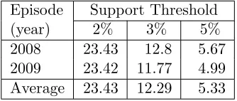
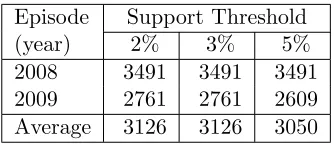
5 Evaluation of The Frequent Pattern Trend Analysis Mechanism 81 5.1 Experimental Analysis of The Trend Identification Module . . . 82
5.1.1 GB Cattle Movement Trend Identification . . . 82
5.1.2 Deeside Insurance Quotation Trend Identification . . . 85
5.1.3 MAF Logistic Cargo Distribution Trend Identification . . . 86
5.1.4 Experimental Analysis of Trend Identification with Constraints . 88 5.1.5 Trend Identification Summary . . . 91
5.2 Experimental Analysis of The Trend Grouping Module . . . 92
5.2.1 GB Cattle Movement Trend Grouping . . . 92
5.2.2 Deeside Insurance Quotation Trend Grouping . . . 97
5.2.3 MAF Logistic Cargo Distribution Trend Grouping . . . 101
5.2.4 Experimental Analysis of Trend Grouping with Constraints . . . 103
5.2.5 Trend Grouping Summary . . . 106
5.3 Experimental Analysis of The Pattern Migration Clustering Module . . 106
5.3.1 GB Cattle Movement Pattern Migration . . . 110
5.3.2 Deeside Insurance Quotation Pattern Migration . . . 112
5.3.3 MAF Logistic Cargo Distribution Pattern Migration . . . 113
5.3.4 Experimental Analysis of Pattern Migration with Constraints . . 113
5.3.5 Pattern Migration Clustering Summary . . . 114
5.4 Experimental Analysis of The Pattern Migration Visualisation Module . 115 5.4.1 GB Cattle Movement Pattern Migration Visualisation and Ani-mation . . . 116
5.4.2 Deeside Insurance Quotation Pattern Migration Visualisation and Animation . . . 120
5.4.3 MAF Logistic Cargo Distribution Pattern Migration Visualisa-tion and AnimaVisualisa-tion . . . 120
5.4.4 Pattern Migration Visualisation Summary . . . 122
5.5 Summary . . . 123
6 Prediction Modeling 124 6.1 Background . . . 125
6.1.1 CTS Frequent Patterns and Trends . . . 125
6.1.2 Prediction Modeling overview . . . 127
6.2.1 Filtering The Frequent Patterns . . . 129
6.2.2 Probability and Percolation Matrices . . . 129
6.3 Visualisation Module . . . 131
6.3.1 The Visuset Prediction Map Tool . . . 131
6.3.2 The Geographical Map tool . . . 132
6.4 Drilling Down . . . 133
6.5 Experimental Analysis of The Prediction Modeling . . . 133
6.5.1 Frequent Patterns Selection . . . 134
6.5.2 Percolation Matrix . . . 134
6.5.3 Visualisation of Prediction Modeling . . . 136
6.5.4 Evaluation of the “Drill-down” Process With Respect To Specific Areas . . . 143
6.6 Summary . . . 146
7 Conclusion 155 7.1 Summary . . . 155
7.2 Main Findings . . . 156
7.3 Research Contributions . . . 159
7.4 Research Future Direction . . . 159
A Probability Maps for CTS Type 1 Combination Patterns between
June and December 2003 161
B Probability Maps for CTS Type 1 Combination Patterns between
February and December 2004 165
C Probability Maps for CTS Type 1 Combination Patterns between
February and December 2005 171
D Probability Maps for CTS Type 1 Combination Patterns between
February and December 2006 177
E Probability Maps for CTS Type 2 Combination Patterns between
June and December 2003 183
F Probability Maps for CTS Type 2 Combination Patterns between
February and December 2004 187
G Probability Maps for CTS Type 2 Combination Patterns between
H Probability Maps for CTS Type 2 Combination Patterns between
February and December 2006 199
List of Figures
1.1 The Conceptual Model of the Proposed Predictive Trend Mining
Frame-work . . . 6
2.1 P-tree generation . . . 22
2.2 Internal representation of P-tree generated in Figure 2.1 . . . 23
2.3 T-tree generation . . . 24
2.4 Types of trends . . . 30
2.5 Significant Change Points in a Trend. . . 31
2.6 A view of 4×4 nodes with nweights . . . 34
2.7 Comparison of Facebook and MySpace growth [86] . . . 37
3.1 (Styalised) Simple Star Network . . . 45
3.2 (Stylaised) Complex Star Network . . . 45
3.3 Discretisation and normalisation CTS attributes . . . 49
3.4 Discretisation and normalisation Deeside Insurance quotation attributes 49 3.5 Discretisation and normalisation MAF Logistic Cargo distribution at-tributes . . . 50
4.1 Schematic illustrating the operation of the FPTA . . . 54
4.2 Structure of TM-tree . . . 56
4.3 A worked example of the operation of the TM-TFP Algorithm . . . 60
4.4 An example of the diagnostic output from the TM-TFP algorithm com-prising a list of frequent patterns and 12 months of trend values . . . 61
4.5 SOM Prototype and Trend lines maps . . . 63
4.6 Prototype map with 7×7 map nodes . . . 74
4.7 Prototype map with 10×10 map nodes . . . 75
4.8 Prototype map with 12×12 map nodes . . . 76
4.9 Trend line map with 7×7 map nodes . . . 77
4.10 Trend line map with 10×10 map nodes . . . 78
4.11 Trend line map with 12×12 map nodes . . . 79
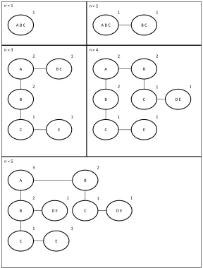
4.12 Four Node Example Network . . . 80
4.14 Three Node Example Network Showing Pattern Migrations fromT1 toT2 80
4.15 Three Node Example Network with Irrelevant links Removed . . . 80
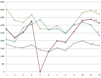
5.1 Trend lines for the CTS Frequent Patterns given in Table 5.3 . . . 85
5.2 Trend lines for the Deeside Insurance Frequent Patterns given in Table 5.6 88 5.3 Trend lines for the MAF Logistic Cargo Frequent Patterns given in Table 5.6 . . . 90
5.4 Trend Grouping module run time (minutes) for the CTS, Deeside Insur-ance and MAF Logistic Cargo networks . . . 93
5.5 CTS network prototype map generated using 2003 episode . . . 94
5.6 CTS network Trend line Map for 2003 episode . . . 95
5.7 CTS network Trend line Map for 2004 episode . . . 96
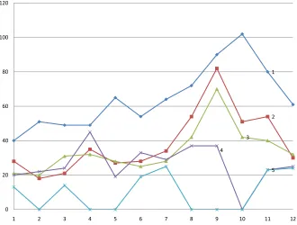
5.8 CTS network number of trends per SOM node per episode . . . 97
5.9 Deeside Insurance network prototype map generated using 2008 episode 98 5.10 Deeside Insurance network Trend line Map for 2008 episode . . . 99
5.11 Deeside Insurance network Trend line Map for 2009 episode . . . 100
5.12 Deeside Insurance network number of trends per SOM node per episode 101 5.13 MAF Logistic Cargo network prototype map generated using 2008 episode102 5.14 MAF Logistic Cargo network Trend line Map for 2008 episode . . . 104
5.15 MAF Logistic Cargo network Trend line Map for 2009 episode . . . 105
5.16 MAF Logistic Cargo network number of trends per SOM node per episode106 5.17 CTS network prototype map with Constraint1 . . . 107
5.18 Deeside Insurance network prototype map for trends with Constraint1 . 108 5.19 Pattern Migration Clustering module run time (seconds) for the CTS, Deeside Insurance and MAF Logistic Cargo networks . . . 109
5.20 Pattern Migration Visualisation module run time (seconds) for the CTS, Deeside Insurance and MAF Logistic Cargo networks . . . 116
5.21 Visusetvisualisation (map) indicating migration of CTS patterns from episode 2003 to episode 2004 . . . 117
5.22 Visusetvisualisation (map) indicating migration of CTS patterns from episode 2004 to episode 2005 . . . 118
5.23 Visusetvisualisation (map) indicating migration of CTS patterns from episode 2005 to episode 2006 . . . 119
5.24 Visusetvisualisation (map) indicating migration of Deeside Insurance patterns from episode 2008 to episode 2009 . . . 121
5.25 Visusetvisualisation (map) indicating migration of MAF Logistic Cargo patterns from episode 2008 to episode 2009 . . . 122
6.1 Simplified view of a map presenting 25 grid square locations . . . 127
6.3 Conceptual Example of the Percolation of Information and Events in a
network fragment . . . 128
6.4 An example of a Probability Map using the network fragment given in Figure 6.3 . . . 131
6.5 The Percolation Matrix run time values (seconds) comparison . . . 135
6.6 January 2003 Type 1 Combination Patterns Probability Map . . . 138
6.7 February 2003 Type 1 Combination Patterns Probability Map . . . 139
6.8 March 2003 Type 3 Combination Patterns Probability Map . . . 140
6.9 April 2003 Type 1 Combination Patterns Probability Map . . . 141
6.10 May 2003 Type 1 Combination Patterns Probability Map . . . 142
6.11 January 2003 Type 2 Combination Patterns Probability Map . . . 143
6.12 February 2003 Type 2 Combination Patterns Probability Map . . . 143
6.13 March 2003 Type 2 Combination Patterns Probability Map . . . 144
6.14 April 2003 Type 2 Combination Patterns Probability Map . . . 144
6.15 May 2003 Type 2 Combination Patterns Probability Map . . . 145
6.16 January 2003 Type 3 Combination Patterns Probability Map . . . 145
6.17 February 2003 Type 3 Combination Patterns Probability Map . . . 145
6.18 March 2003 Type 3 Combination Patterns Probability Map . . . 146
6.19 April 2003 Type 3 Combination Patterns Probability Map . . . 146
6.20 Location areas of January-February 2003 Type 1 Combination Patterns of Cattle Movement . . . 147
6.21 January 2004 Type 1 Combination Patterns Probability Map . . . 148
6.22 January 2005 Type 1 Combination Patterns Probability Map . . . 149
6.23 January 2006 Type 1 Combination Patterns Probability Map . . . 150
6.24 January 2004 Type 2 Combination Patterns Probability Map . . . 151
6.25 January 2005 Type 2 Combination Patterns Probability Map . . . 152
6.26 January 2006 Type 2 Combination Patterns Probability Map . . . 152
6.27 “Drill-down” version of January 2005 Type 1 Combination Patterns Probability Map . . . 153
6.28 “Drill-down” version of February 2005 Type 1 Combination Patterns Probability Map . . . 154
A.1 June 2003 Type 1 Combination Patterns Probability Map . . . 161
A.2 July 2003 Type 1 Combination Patterns Probability Map . . . 162
A.3 August 2003 Type 1 Combination Patterns Probability Map . . . 162
A.4 September 2003 Type 1 Combination Patterns Probability Map . . . 163
A.5 October 2003 Type 1 Combination Patterns Probability Map . . . 163
A.6 November 2003 Type 1 Combination Patterns Probability Map . . . 164
B.1 February 2004 Type 1 Combination Patterns Probability Map . . . 165
B.2 March 2004 Type 1 Combination Patterns Probability Map . . . 166
B.3 April 2004 Type 1 Combination Patterns Probability Map . . . 166
B.4 May 2004 Type 1 Combination Patterns Probability Map . . . 167
B.5 June 2004 Type 1 Combination Patterns Probability Map . . . 167
B.6 July 2004 Type 1 Combination Patterns Probability Map . . . 168
B.7 August 2004 Type 1 Combination Patterns Probability Map . . . 168
B.8 September 2004 Type 1 Combination Patterns Probability Map . . . 169
B.9 October 2004 Type 1 Combination Patterns Probability Map . . . 169
B.10 November 2004 Type 1 Combination Patterns Probability Map . . . 170
B.11 December 2004 Type 1 Combination Patterns Probability Map . . . 170
C.1 February 2005 Type 1 Combination Patterns Probability Map . . . 171
C.2 March 2005 Type 1 Combination Patterns Probability Map . . . 172
C.3 April 2005 Type 1 Combination Patterns Probability Map . . . 172
C.4 May 2005 Type 1 Combination Patterns Probability Map . . . 173
C.5 June 2005 Type 1 Combination Patterns Probability Map . . . 173
C.6 July 2005 Type 1 Combination Patterns Probability Map . . . 174
C.7 August 2005 Type 1 Combination Patterns Probability Map . . . 174
C.8 September 2005 Type 1 Combination Patterns Probability Map . . . 175
C.9 October 2005 Type 1 Combination Patterns Probability Map . . . 175
C.10 November 2005 Type 1 Combination Patterns Probability Map . . . 176
C.11 December 2005 Type 1 Combination Patterns Probability Map . . . 176
D.1 February 2006 Type 1 Combination Patterns Probability Map . . . 177
D.2 March 2006 Type 1 Combination Patterns Probability Map . . . 178
D.3 April 2006 Type 1 Combination Patterns Probability Map . . . 178
D.4 May 2006 Type 1 Combination Patterns Probability Map . . . 179
D.5 June 2006 Type 1 Combination Patterns Probability Map . . . 179
D.6 July 2006 Type 1 Combination Patterns Probability Map . . . 180
D.7 August 2006 Type 1 Combination Patterns Probability Map . . . 180
D.8 September 2006 Type 1 Combination Patterns Probability Map . . . 181
D.9 October 2006 Type 1 Combination Patterns Probability Map . . . 181
D.10 November 2006 Type 1 Combination Patterns Probability Map . . . 182
D.11 December 2006 Type 1 Combination Patterns Probability Map . . . 182
E.1 June 2003 Type 2 Combination Patterns Probability Map . . . 183
E.2 July 2003 Type 2 Combination Patterns Probability Map . . . 184
E.3 August 2003 Type 2 Combination Patterns Probability Map . . . 184
E.5 October 2003 Type 2 Combination Patterns Probability Map . . . 185
E.6 November 2003 Type 2 Combination Patterns Probability Map . . . 186
E.7 December 2003 Type 2 Combination Patterns Probability Map . . . 186
F.1 February 2004 Type 2 Combination Patterns Probability Map . . . 187
F.2 March 2004 Type 2 Combination Patterns Probability Map . . . 188
F.3 April 2004 Type 2 Combination Patterns Probability Map . . . 188
F.4 May 2004 Type 2 Combination Patterns Probability Map . . . 189
F.5 June 2004 Type 2 Combination Patterns Probability Map . . . 189
F.6 July 2004 Type 2 Combination Patterns Probability Map . . . 190
F.7 August 2004 Type 2 Combination Patterns Probability Map . . . 190
F.8 September 2004 Type 2 Combination Patterns Probability Map . . . 191
F.9 October 2004 Type 2 Combination Patterns Probability Map . . . 191
F.10 November 2004 Type 2 Combination Patterns Probability Map . . . 192
F.11 December 2004 Type 2 Combination Patterns Probability Map . . . 192
G.1 February 2005 Type 2 Combination Patterns Probability Map . . . 193
G.2 March 2005 Type 2 Combination Patterns Probability Map . . . 194
G.3 April 2005 Type 2 Combination Patterns Probability Map . . . 194
G.4 May 2005 Type 2 Combination Patterns Probability Map . . . 195
G.5 June 2005 Type 2 Combination Patterns Probability Map . . . 195
G.6 July 2005 Type 2 Combination Patterns Probability Map . . . 196
G.7 August 2005 Type 2 Combination Patterns Probability Map . . . 196
G.8 September 2005 Type 2 Combination Patterns Probability Map . . . 197
G.9 October 2005 Type 2 Combination Patterns Probability Map . . . 197
G.10 November 2005 Type 2 Combination Patterns Probability Map . . . 198
G.11 December 2005 Type 2 Combination Patterns Probability Map . . . 198
H.1 February 2006 Type 2 Combination Patterns Probability Map . . . 199
H.2 March 2006 Type 2 Combination Patterns Probability Map . . . 200
H.3 April 2006 Type 2 Combination Patterns Probability Map . . . 200
H.4 May 2006 Type 2 Combination Patterns Probability Map . . . 201
H.5 June 2006 Type 2 Combination Patterns Probability Map . . . 201
H.6 July 2006 Type 2 Combination Patterns Probability Map . . . 202
H.7 August 2006 Type 2 Combination Patterns Probability Map . . . 202
H.8 September 2006 Type 2 Combination Patterns Probability Map . . . 203
H.9 October 2006 Type 2 Combination Patterns Probability Map . . . 203
H.10 November 2006 Type 2 Combination Patterns Probability Map . . . 204
List of Tables
2.1 A possible classification of spatial temporal DM tasks and techniques [141] 29
3.1 Examples of discretisation and normalisation of data attributes . . . 48
4.1 Number of trends identified using TM-TFP for a sequence of four GB
Cattle Movement network episodes and a range of support thresholds . 61
4.2 Start Condition . . . 68
4.3 First Iteration . . . 68
4.4 Second Iteration . . . 68
4.5 Pattern Migration Summary for Example Network Given in Figure 4.14 71
4.6 C-value (Correlation Coefficient) Calculation for Example Network Given
in Figure 4.14 . . . 72
5.1 Number of trends identified using TM-TFP for a sequence of four CTS
network episodes and a range of support thresholds . . . 83
5.2 The TM-TFP algorithm run time values (seconds) using the CTS social
network episodes . . . 83
5.3 Example frequent patterns and associated trends obtained from the 2003
CTS network using a 0.5% minimum support threshold . . . 84
5.4 Number of frequent pattern trends identified using the Deeside Insurance
network and a range of support thresholds . . . 86
5.5 The TM-TFP algorithm run time values (seconds) using the Deeside
Insurance social network . . . 86
5.6 Example frequent patterns and associated trends obtained from the 2008
Deeside Insurance network using a 5% minimum support threshold . . . 87
5.7 Number of frequent pattern trends identified using the MAF Logistic
Cargo network and a range of support thresholds . . . 87
5.8 The TM-TFP algorithm run time values (seconds) using the MAF
Lo-gistic Cargo network network . . . 87
5.9 Example frequent patterns and associated trends obtained from the 2008
MAF Logistic Cargo network using a 5% minimum support threshold . 89
5.11 Number of identified trends using Deeside Insurance network . . . 91
5.12 Format of a Migration Matrix . . . 110
5.13 Example of migrating CTS Frequent Patterns trends . . . 111
5.14 Fragment of the pattern Migration Matrix fromM2003 node (cluster) to M2004 for the CTS network dataset . . . 111
5.15 Example of migrating Deeside Insurance Frequent Patterns trends . . . 112
5.16 Fragment of the pattern Migration Matrix from M2008 toM2009 for the
Deeside Insurance network dataset . . . 113
5.17 Example of migrating MAF Logistic Cargo Frequent Patterns trends . . 114
5.18 Fragment of pattern Migration Matrix fromM2008 toM2009 for the MAF
Logistic Cargo network dataset . . . 114
5.19 Examples of migrating CTS trends with constraints (Dist = distance
value) . . . 115
5.20 Examples of migrating Deeside Insurance trends with constraints (Dist
= distance value) . . . 115
6.1 An example of a Percolation Matrix using the network fragment given
in Figure 6.3 . . . 130
6.2 Sample of 2003 CTS Type 2 combination pattern Monthly Probabilities 135
6.3 Sample of 2004 CTS Type 2 combination pattern Monthly Probabilities 136
6.4 Definition of Example Location Area Grid IDs in Terms of Eastings and
Northings . . . 136
6.5 January 2004 Type 2 Percolation Matrix indicating the probability of an
Acknowledgement
First and foremost, my greatest debt of gratitude must go to my first supervisor, Dr.
Frans Coenen. He patiently provided the supervision, encouragement, constructive
criticism, research ideas and advice to proceed through the PhD program and
com-plete my thesis. I also would like to express my appreciation to my second supervisor,
Dr. Rob Christley, for his support, suggestions and valuable comments.
I am also thankful to Christian Setzkorn. Christian has been helpful in providing
advice many times during my research work. I also would like to extend great
appre-ciation to Dr. Wataru Sunayama for his valuable collaboration.
I also extend my gratitude to the Ministry of Higher Education and Universiti
Per-tahanan Nasional Malaysia for the financial support that has given me the opportunity
to undergo the PhD program.
The best and worst moments of my doctoral journey have been shared with many
people. It has been a great privilege to spend several years in the Department of
Com-puter Science at University of Liverpool, and its staff members will always remain dear
to me. My colleagues and friends, Ayu, Zurina, Zuraini, Rina, Stephanie, Santhana,
Hanafi, Matt and the rest, thank you for the support and suggestions.
I wish to thank my parents and family especially my beloved sons, Megat Daniel
Arif and Megat Ilhan Arif. Their love provided my inspiration and was my driving
force to complete my PhD. My sister, Puteri Nor Alaina, thanks to her for all her love,
Chapter 1
Introduction
Data Mining (DM) is a generic term used to describe processes used to achieve the
automated analysis (by computer) of data with the aim of discovering hidden knowledge
[51]. DM is an element in the Knowledge Discovery in Data (KDD) process. KDD
encompasses a set of techniques that include, for example, data warehousing, data
pre-processing and post-processing; as well as DM. DM has many applications such as:
1. Bank and financial industry data analysis, where it is used to minimize fraud
and identify high risk or bad customers [5, 20], and to attempt to forecast stock
market movement [124].
2. Medical research, where it is used to monitor (for example) the growth of cancer
cell patterns in patients [35].
3. Retail industry support, where it is used to develop marketing and stock
replen-ishment strategies based on customer behaviour and purchasing patterns [15].
4. Telecommunication and computer network analysis, where it is used to identify
the loyalty of (say) mobile subscribers in terms of churn rate [47, 104], and to
detect network intrusions or irregular behaviour with respect to network users
[17, 37].
DM encompasses a variety of techniques such as classification, clustering and
pat-tern discovery. The work described in this thesis is predominantly directed at the latter.
In pattern discovery the patterns of interest may take many forms, such as frequently
occurring word groups that may exist across a document collection or frequently
oc-curring sub-graphs in graph data. More commonly the frequent patterns of interest are
simply frequently occurring sub-sets of attribute values that occur together in tabular
datasets. The extraction of frequent patterns from data is typically computationally
expensive because, given any reasonably sized dataset, there tends to be a large number
of potential frequent patterns. Given nbinary valued attributes there are potentially
The amount of data available for the application of data mining has increased
rapidly over recent years. Reasons for this include the availability of inexpensive storage
and increases in the capabilities of computer hardware. In parallel to the increase in the
amount of data collected there has been a corresponding increase in the desire to apply
data mining techniques to this data. There is also an increasing interest in studying
the spatiality and temporality of the data as this may provide further interesting and
useful insights. One element of the latter is trend mining, where we wish to identify
how patterns change with time (or do not change).
In the work described in this thesis a trend is conceptualized as a time series
com-prising a sequence of “occurrence” values plotted against time. More specifically the
author is interested in identifying temporal trends in networks such as social and
distri-bution networks. Social networks represent the interaction among individuals in some
social setting; the nodes in the network typically represent the individuals and the links
the interactions. In distribution networks the nodes describe locations (which might be
individuals) and the links the “traffic” between locations. Networks, although typically
conceived of in terms of graphs, can also be represented in a tabular format such that
each record represents a time stamped “interaction” between two nodes. As such
tab-ular pattern mining techniques can be used to identify patterns in a tabulated “snap
shot” of a network. If we then take a sequence of snap shots we can mine trends in the
data by identifying changes in the patterns over time. Given that, as noted above,
fre-quent pattern mining typically results in a large number of patterns a significant issue
in such trend analysis is the large number of frequent patterns and trends that may
be discovered. To address this issue this thesis describes an overall frequent pattern
trend mining and analysis mechanism. The proposed framework is designed to identify
frequent pattern trends and also provide mechanisms to group and analyse large
num-ber of frequent pattern trends. The proposed trend analysis is directed at detecting
changes in a sequence of identified frequent pattern trends. This thesis also considers
additional analytical techniques, including visualisation and prediction techniques. The
visualisation technique provides assistance for users to interpret trend analysis results.
Finally the prediction technique uses knowledge of trends to support the investigation
of the movement of patterns within social networks.
The rest of this introductory chapter is organized as follows. In Section 1.1 the
motivation for the research is discussed. Section 1.2 presents the research question and
associated issues. In Section 1.3 the programme of work is outlined. Then Section 1.4
discusses the criteria used to evaluate the research outcomes (the “criteria for success”)
followed in Section 1.5 with detail of the “contribution” of the research. Section 1.6,
then presents an outline of the structure of the remainder of the thesis, followed in
Section 1.7 with details of published work produced as a result of the described research.
1.1
Research Motivation
Trends provide useful information for decision and policy makers. For example
knowl-edge of seasonal trends in customer buying patterns, trends describing change in the
behaviour of social networking site users, and trends on how some disease or condition
might spread in a given geographical area, are all potentially useful to decision makers.
The discovery of interesting trends helps us to detect dynamic changes in data that can
lead to actions being taken and/or policy or regulation amendments.
The motivation for the research described in this thesis can thus be broadly
iden-tified as the desire to realise the advantages that frequent pattern trend mining can
offer to support decision makers. More specifically, in this thesis a number of
spe-cific applications are considered in detail: (i) The cattle movement tracking system in
operation in Great Britain (GB), (ii) an online insurance quote system operated by
Deeside Insurance Ltd and (iii) the logistics network operated by the Malaysian Armed
Forces. It is suggested that analysis of the GB cattle movement network provides trend
knowledge useful for policy and decision makers who wish to monitor and address
is-sues such the spread of cattle disease. Similarly the analysis of the Deeside Insurance
dataset provides useful knowledge with respect to customer behaviour to support
mar-keting initiatives. Trend interpretation within the Malaysian Armed Forces Logistic
Cargo network provides for logistic item stock management and distribution pattern
monitoring over time. Further details of these datasets are presented later in this thesis.
1.2
Research Issues and Question
Given the above the key aim of the work described in this thesis is to research and
investigate effective mechanisms to: (i) discover temporal frequent patterns and trends
in network data, and (ii) facilitate the analysis of these trends and patterns to predict
behaviour across networks. Realisation of this aim requires the solution of a number of
research issues:
1. Frequent Patterns and Trends: How can we represent frequent patterns and trends so as to facilitate the desired trend mining? How do we transform the raw
datasets to support the mining process? Given a large quantity of temporal data,
how do we handle the granularity of the time stamps? How do we represent and
highlight the trends as a time series result?
2. Change Detection: How can we detect changes in the identified trends? How do we define the types of changes that we are interested in? How do we measure
the degree of these changes?
patterns and trends? How do we measure the interestingness of these patterns and
trends? Can we apply constraints to the data to anticipate interesting, desirable
and useful patterns and trends?
4. Interpretation of Patterns and Trends: How do we interpret types of fre-quent pattern trends to the users? How do we annotate the changes occurred in
frequent pattern trends in the mining and analysis process?
5. Prediction: How can we predict the “percolation” of information within a net-work? Can we use the discovered patterns and trends to predict the probability
of any activity or event in the network? If prediction is possible, what methods
are best to manipulate the patterns and trends?
6. Visualization: How can we visualize the findings to enhance user understand-ing? What are the suitable interfaces/features for projecting the results? What
methods are best suited to illustrating the temporality of patterns, and trend
changes and predictions? If spatial patterns are involved, how can we best relate
these patterns to the actual geographical locations?
The overriding research question is thus: “What are the most appropriate mecha-nism for identifying, analyzing and displaying trends in network data; and how might those trends usefully be employed for prediction purposes?” The following section pro-vides a description of the broad research methodology adopted to address this research
question.
1.3
Research Methodology
To act as a focus for the work a social network extracted from the GB cattle movement
database was used. This was selected because: (i) this provided a substantial network,
(ii) it featured time stamps and (iii) analysis of the network would provide an exemplar
of the kind of application where the results of the research could be usefully employed.
As the research progressed two additional datasets were considered: Deeside Insurance
and Malaysian Armed Forces Logistic Cargo. The following programme of work was
adopted:
Representation: Investigation of: (i) mechanisms whereby network data could be represented as tabular data, and (ii) mechanisms for conducting the necessary
preprocessing with respect to the target datasets.
Frequent Pattern Trend Mining: Investigation into mechanisms to identify the de-sired trends. The intention here was to build a frequent pattern trend mining
system that could be analysed and evaluated, and which could then be used as
Trend Clustering: The identification of some mechanism whereby the anticipated large number of identified trends could be grouped so as to facilitate
understand-ing. The intention here was to use some form of SOM to achieve the desired
clustering.
Change Detection: The investigation of techniques whereby changes in trends (or the absence of changes) could be identified. The fundamental idea here was to
research mechanisms whereby a sequence of self organizing maps could be related
and thus trend movements from one cluster to another identified.
Visualisation: Having identified changes in pattern trends it was felt to be desirable to have some mechanism for displaying this to end users. An investigation into
a strategy whereby pattern changes could be visualized was therefore deemed
desirable.
Prediction: Given knowledge of the pattern trends that exist within a network data collection the final phase in the programme of work was concerned with an
in-vestigation of how this knowledge might be used to predict the progress of some
event across the network.
It was deemed desirable to incorporate the above elements into some forms of
inte-grated framework, a particular artifact resulting from the proposed programme of work
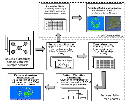
is therefore the Predictive Trend Mining Framework (PTMF). Figure 1.1 illustrates the
conceptual model of the PTMF which consists of two parts: (i) Frequent Pattern Trend
Analysis and (ii) Prediction Modeling. The Frequent Pattern Trend Analysis part has
four modules to identify and analyse the frequent patterns and trends that may be
con-tained within a network dataset. The Prediction Modeling part comprises two modules
to determine and predict the probability of future activities in a social network.
1.4
Evaluation Criteria
This section discusses the evaluation criteria used to measure the quality of the research
undertaken in the context of the above programme of work. The aim was to develop
criteria that could be usefully employed to determine the effectiveness of techniques
proposed to address the various identified research issues. The following requirements
were therefore considered:
1. Genericity. Any proposed technique was required to be generic so that it would have general applicability, thus allowing for the analysis of different forms of social
network data, from www usage data to business community data. Genericity was
demonstrated by applying proposed techniques to a variety of social network data
Percolation Matrix
Calculating probability of information movement between network nodes.
1 2 3 4 5 6 1 0.00 0.00 0.00 0.01 0.00 0.00 2 0.00 0.00 0.00 0.01 0.00 0.00 3 0.00 0.01 0.00 0.00 0.00 0.00 4 0.00 0.00 0.01 0.01 0.00 0.00 5 0.00 0.00 0.00 0.04 0.00 0.00 6 0.00 0.00 0.00 0.01 0.03 0.00
Prediction Modeling Visualisation
Visualisation of Prediction Modeling in Social Network
Data input, describing collection of n time stamped networks
Prediction Modeling
[image:22.612.115.545.67.404.2]Frequent Pattern Trend Analysis
Figure 1.1: The Conceptual Model of the Proposed Predictive Trend Mining Framework
2. Computational time and memory. Most frequent pattern mining algorithms are computationally expensive. As the size of the dataset increases, the
computa-tional and memory resource required increases significantly. Any potential trend
mining and analysis technique should therefore be able to process large
num-bers of records in reasonable time. Run time and memory usage measurements
were therefore used as a mechanism for determining the effectiveness of proposed
techniques.
3. Flexibility and Reusability. Regardless of their specific nature trend mining and analysis mechanisms should be able to adapt to accommodate different types
of datasets. For example any proposed algorithm should be able to accommodate
further features. It also should be able to accept data attribute selections and
data constraints to reflect individual user interests. Users should also be able to
conduct the desired trend mining with different levels of granularity; for example
weekly, monthly and yearly. Flexibility and reusability was tested using different
4. Scalability. Any proposed technique, to be considered genuinely useful, should be scalable, i.e. it should be able to operate with large datasets. Thus datasets
featuring substantial numbers of records and/or attributes were used to evaluate
the proposed techniques.
5. Accuracy. Clearly the proposed technique should also discover the correct pat-terns and trends. This was established, using the cattle movement database,
through consultation with domain experts.
As already noted, for evaluation purposes several real world and diverse network
datasets were used: (i) GB cattle movement, (ii) Deeside Insurance quotes and (iii)
Malaysian Armed Forces logistic cargo distribution.
1.5
Research Contributions
The main contributions of the research work considered in this thesis can be summarized
as follows:
1. A mechanism for efficiently generating temporal spatial frequent patterns and
trends, that may exist within networks, in terms of episodes or epochs (this will
be explained in further detail later in this thesis).
2. A mechanism for clustering groups of trends, using a SOM technique, so as to
assist in the further analysis of the identified trends.
3. A trend cluster analysis mechanism to support the detection of changes in trends
and frequent pattern migrations.
4. A visualization of pattern movement (traffic) from one trend cluster to another
over a period of time, again to facilitate and support trend analysis.
5. A prediction modeling and visualisation technique that can be applied to network
data, which illustrates the manner in which information (events) might travel
across a (social) network.
1.6
Structure of Thesis
The rest of this thesis is organized as follows:
Chapter 2 presents a literature review of the related research on data mining and KDD, frequent pattern and temporal mining, social network and trend analysis,
Chapter 3 presents a brief description of the selected network datasets. As already noted three network datasets were used for the experiments: (i) the GB cattle
movement data, (ii) Deeside Insurance quotation data and (iii) Malaysian Armed
Forces (MAF) logistic cargo distribution data. The GB cattle movement data
has been used as the main dataset for the experiments, the latter two were used
to confirm the genericity, flexibility and reusability of the proposed algorithms.
Chapter 4 presents the proposed modules for the Frequent Pattern Trend Analysis which is the first part of the PTMF. This includes mechanisms to generate
fre-quent patterns and trends, cluster similar groups of trends and detect changes
in frequent patterns and trends over a period of time. This part of the
frame-work consists of four modules (Figure 1.1), (i) the Trend Identification module
to mine frequent patterns and trends using the Trend Mining-Total From Partial
algorithm, (ii) the Trend Grouping module to group large numbers of discovered
trends to ease the process of trend analysis, (iii) the Pattern Migration
Cluster-ing module to analyse the temporal pattern movement from one trend cluster to
another and to identify communities of clusters of pattern migrations, and (iv)
the Pattern Migration Visualisation module designed to provide a mechanism for
illustrating trend changes and pattern migrations to end users.
Chapter 5 presents an evaluation of the proposed modules for the Frequent Pattern Trend Analysis which were introduced in Chapter 4, from pattern and trend
iden-tification to the visualisation of pattern migrations. The evaluation was conducted
with respect to the criteria identified in Sub-section 1.4 above.
Chapter 6 introduces the Prediction Modeling technique. The technique comprises several elements to predict the “percolation” of information and events in a
net-work given specific frequent patterns. The framenet-work also includes a visualization
tool to provide an animation of the percolation. In this case the experiments were
performed using the frequent patterns generated using the GB cattle movement
data only. A series of experiments were undertaken to demonstrate how the
percolation of information and events in a social network can be predicted. A
mechanism to support the “drilling down” into trend data is also considered.
Chapter 7 concludes the thesis and presents a summary of the work presented and the main findings in terms of the identified research question and issues. The
chapter also includes a discussion on possible directions for a future work.
1.7
Published Work
Some of the work described in this thesis has been the subject of number of refereed
1. Journal Papers
(a) Nohuddin, P.N.E., Coenen, F., Christley, R., Setzkorn, C., Patel, Y. and Williams, S. Finding “Interesting” Trends in Social Networks Using Fre-quent Pattern Mining and Self Organizing Maps. Knowledge Based System Journal 2011. Journal article comprising an extended, updated and re-vised version of conference paper (f) below, which described parts of the
experimental analyses using the GB cattle movement and Deeside Insurance
databases presented in Sections 5.1, 5.2 and 5.3 included in Chapter 5 of
this thesis. Frans Coenen is the main supervisor and Rob Christley is the
co-supervisor who is also the domain expert with respect to the GB cattle
movement database. Yogesh Patel and Shane Williams are the advisors from
the Deeside Insurance Ltd. Christian Setzkorn provided additional advise
on the processing of the data.
(b) Nohuddin, P.N.E., Sunayama, W., Coenen, F., Christley, R. and Setzkorn, C. Trend Mining in Social Networks: From Trend Identification to Visuali-sation. It has been submitted to Expert Systems: the Journal of Knowledge Engineering 2012. This is an extended version of conference paper(g) be-low that summarised the proposed modules for the Frequent Pattern Trend
Analysis process described in Sub-sections 4.3, 4.4, 4.5 and 4.6 included in
Chapter 4 of this thesis. The journal also included details of the GB
cat-tle movement pattern trend analysis addressed in Sub-sections 5.1.1, 5.2.1,
5.3.1 and 5.4.1 of Chapter 5. Wataru Sunayama is the Visuset advisor from
Hiroshima City University.
2. Conference Papers
(c) Nohuddin, P.N.E., Coenen, F., Christley, R. and Setzkorn, C. Trend Min-ing in Social Networks: A Study UsMin-ing A Large Cattle Movement Database. ICDM, Springer-Verlag Berlin, Heidelberg (2010). Conference paper report-ing on some initial work on trend minreport-ing that proposed a trend minreport-ing
mech-anism, founded on frequent pattern mining (the TFP-TM algorithm) and
clustering (Sections 5.1 and 5.2 of Chapter 4 of this thesis cover this aspect of
the work), to identify temporal spatial trends in social networks. The work
was illustrated using the GB cattle movement database (see Sub-sections 5.1.1
and 5.2.1 of Chapter 5).
built on work described in (c) and included additional work to detect cluster
changes in social networks. The GB cattle movement database (described in
Section 3.1 in Chapter 3) was again used in the evaluation section. Trend
analysis was done using a distance function to highlight temporal cluster
change (described in Sub-sections 5.1.1, 5.2.1 and 5.3.1 of Chapter 5).
(e) Nohuddin, P.N.E., Coenen, F., Christley, R., Setzkorn, C., Patel, Y. and William, S. Frequent Pattern Trend Analysis in Social Networks. ADMA’10 Proceedings of the 6th International Conference on Advanced data mining and applications: Part I, Springer-Verlag Berlin, Heidelberg (2010). The paper described an extension of work described in (d) whereby constraints were
applied to the mining process so as to enhance the trend analysis results.
The evaluation section reported on experiments using the Deeside Insurance
quotation database as well as the GB cattle movement database used
previ-ously. The material covered in this paper has been included and extended in
Sub-sections 5.1.4, 5.2.4 and 5.3.4 of Chapter 5.
(f) Nohuddin, P.N.E., Coenen, F., Christley, R., Setzkorn, C., Patel, Y. and Williams, S. Social Network Trend Analysis Using Frequent Pattern Mining and Self Organizing Maps. AI-2010: SGAI International Conference. pp 311-324 (2010). The paper reported on a technique for identifying, grouping and analyzing trends in social networks using a cluster analysis strategy to
identify “interesting” trends (similar work is presented in Sections 5.1, 5.2 and
5.3 of Chapter 5). The study focused on two types of network, star networks
and complex star networks, exemplified by two real applications: the GB
cattle movement and the Deeside Insurance quotation databases which are
described in Sections 3.1 and 3.2 of Chapter 3.
(g) Nohuddin, P.N.E., Sunayama, W., Coenen, F., Christley, R. and Setzkorn, C. Trend Mining and Visualisation in Social Networks. AI 2011: SGAI Inter-national Conference on Artificial Intelligence. Conference paper describing an updated trend mining framework to that published previously, the IGCV
(Identification, Grouping, Clustering and Visualisation) framework that
in-troduced the proposed visualisation mechanism (Sub-sections 4.3, 4.4, 4.5
and 4.6 of Chapter 4). Evaluation of its operation was reported using the GB
cattle movement network; the evaluation is reported in an extended manner
in Sub-sections 5.1.1, 5.2.1, 5.3.1 and 5.4.1 of Chapter 5. This paper won the
prize for the Best Student Paper award.
2012: The Pacific Rim International Conference on Artificial Intelligence (PRICAI). Conference paper that described the Pattern Migration Identifi-cation and Visualisation (PMIV) framework which was designed to operate
using trend clusters, extracted from large network data using a Self
Organ-ising Map technique. The PMIV framework was also used to facilitate the
detection of changes in the characteristics of trends over time, and
“commu-nities” of trend clusters. The content of this paper has been used to form
the foundation of the material presented in Sections 4.5 and 4.6 included in
Chapter 4 of this thesis. Evaluation of its operation was reported using the
GB cattle movement network (similar evaluation is presented in Sub-sections
5.3.1 and 5.4.1 of Chapter 5).
1.8
Summary
In summary, this chapter has provided an overview and background for the research
described in the remainder of this thesis, including details concerning the motivation for
the work and the research question and issues. It has also provided a brief description
of the programme of work, the research evaluation criteria and the contribution of the
work. In the following chapter a literature review, intended to provide much more detail
Chapter 2
Literature Review
As noted in Chapter 1, the research described in this thesis seeks to establish an effective
mechanism to identify and group trends found in social network data, and also to
facilitate the analysis of these trends with respect to network activity. In addition,
the research is directed towards the presentation of the analysis using some form of
visualisation. This chapter reviews the relevant previous work on which the proposed
framework to realise the desired thesis aims is founded.
This chapter is organized into eight sub-topics as follows: (i) Knowledge Discovery
in Databases (KDD) and Data Mining, (ii) Association Rules and Frequent Pattern
Mining, (iii) Temporal and Spatial Data Mining, (iv) Trend Mining, (v) Clustering
Techniques, (vi) Social Network Analysis and Mining, (vii) Prediction Modeling and
(viii) Visualization. Each sub-topic is considered in a separate Section. Section 2.1
elaborates on the concept and process of KDD and distinguishes between KDD and
Data Mining. Section 2.2 describes the concept of Association Rules and Frequent
Pattern Mining (FPM) and reviews several established FPM algorithms. Sections 2.3
and 2.4 focus on mining techniques using temporal spatial data and trend mining;
Section 2.4 also considers trend analysis. Section 2.5 describes the concept of Clustering,
especially in the context of using Self Organising Maps as a clustering technique, and
reviews some related work on cluster analysis. Section 2.6 discusses the concept of social
networks, and techniques in social network analysis and mining. Section 2.7 evaluates
the concept of prediction modeling in social networks and also considers techniques
which have been introduced to predict events or movement of information (and other
activities) in a network. Section 2.8 then describes related work on visualization in
data mining. Finally Section 2.9 presents a summary of this chapter.
2.1
Knowledge Discovery in Databases and Data Mining
Using current ICT the amount of stored data has accumulated rapidly. Given this
amount of data the assumption is that there is valuable hidden knowledge within this
makers and stakeholders. For example, historical customer bank transaction data may
be used to rank and assess customers. Banks have employed such procedures for many
years as a means of deciding whether or not to approve loans and credit cards.
Com-panies and institutions of all kinds have used similar methods to identify their most
valuable customers.
A variety of tools and methods have been proposed to store data to support business
applications [39, 58, 113]. Many database and data administrators use Structured
Query Language (SQL) and similar tools to maintain and manipulate stored data.
However, such database tools are not able to discover non-trivial hidden information
or knowledge in data, such as relationships and/or causal data attribute patterns.
The identification of such knowledge requires alternative tools; this is the domain of
Knowledge Discover in Data (KDD).
In the research described in this thesis the author focuses on KDD techniques,
specifically data mining tools, directed at data that has been extracted from social
network information. The assumption is that the mining process is done using historical
data which has been transferred from some operational database to a data warehouse.
In this section the concept of KDD is discussed further in Sub-section 2.1.1 and the
KDD process in Sub-section 2.1.2. Data mining, a central element within then KDD
process, is then reviewed in Sub-section 2.1.3.
2.1.1 The Concept of Knowledge Discovery in Databases
The terms Knowledge Discovery in Databases (KDD) and Data Mining (DM) have
been used interchangeably to describe the process of extracting useful and meaningful
information from data. However in this thesis, and in line with many other authors,
KDD is defined as the whole process of discovering useful information and knowledge
within data, whereas DM is defined as the task within the KDD process where tools
and mechanism are applied to identify (mine) the knowledge of interest [39, 42, 43].
The application of KDD is widespread and includes revenue generation, medical and
diseases monitoring and the provision of support for “homeland security”. To give
three specific examples: [72] describes a health case management system to identify
and predict the possible causes whereby a patient may be considered to be a “high
risk” patient; [68] describe a KDD system, to support a social program for children,
founded on the application of KDD to street crime data in Ethiopia; and [138] apply
KDD to a Taiwanese airline passenger database to identify “valued customers”.
KDD incorporates a number of processes, from the preparation of raw data prior
to the application of DM to visualization of the final result. The following sub-section
2.1.2 The KDD Process
As noted above, the KDD process encompasses a number of stages. It is generally
acknowledged [29, 39, 135] that most KDD applications can be divided into five stages
as follows:
1. Problem understanding: During this first stage the scope and boundaries of the KDD problem to be addressed are defined. Discussion with end users and
decision makers is typically undertaken so as to establish the objectives of the
desired KDD. Data is usually collected from various data sources and combined
into a single data repository (data warehouse).
2. Pre-processing: The collected data typically includes anomalies that need to be corrected or removed to avoid inaccurate results. The pre-processing stage
includes the filtering of data records to remove null values, noise reduction and
sometimes the anonimisation of sensitive data.
3. Transformation: Some of the collected data may have different formats from one another, thus in stage three (where necessary) all data is converted to a
standard format.
4. Data Mining: In stage four the actual knowledge discovery takes places using some appropriate data mining technique (the data mining stage is considered in
further detail in the following sub-section).
5. Evaluation: The final stage of the KDD process comprises the analysis of the data mining results (this might include the use of visualisation techniques).
2.1.3 Data Mining
From the above DM can be claimed to be the central activity within the overall KDD
process. DM encompasses the use of tools and techniques to discover knowledge in data.
DM can result in the identification of patterns, associations and relationships of many
forms. Typical DM activities include Association Rule Mining (ARM), Classification,
Clustering, Sequencing and Forecasting [39, 52, 136]. Each is considered in some further
detail below:
1. Association Rule Mining (ARM): ARM is concerned with the discovery of relationships between data attributes. The frequently cited exemplar application
for ARM is supermarket basket analysis (customers who buy eggs are also likely
to buy bread).
2. Classification: Classification is concerned with decision making, the allocation of a current situation to a category (class). A frequently cited exemplar
play golf or not given the current weather conditions (the classes in this case are
“play” and “don’t play”). The classifiers used are generated using what are called
supervised learning methods in that they require pre-labeled training data.
3. Clustering: Clustering is directed at the process of partitioning data records into groups (clusters) that share similar characteristics. In this case the data groups
are not known before hand. Clustering techniques are therefore referred to as
unsupervised learning methods. It is interesting to note that once a set of clusters
have been derived the definition of the clusters can be used for classification
purposes.
4. Sequence Mining: Sequence mining refers to the process of determining the relationships between data attributes according to some ordering (normally a
temporal ordering). The mining process is usually performed using time stamped
data.
5. Forecasting: Forecasting is akin to classification however, it incorporates a tem-poral element. Generally, sequence data is used and some mechanism applied to
predicts future events.
The work described in this thesis incorporates elements of ARM, Clustering,
Se-quence Mining and Forecasting; of which ARM (or Frequent Pattern Mining) is the
most central. The following section therefore considers ARM in more detail.
2.2
Association Rules and Frequent Pattern Mining
This section describes the ideas behind Association Rules (ARs) and the more general
issues associated with Frequent Pattern Mining (FPM). In this thesis FPM is considered
to be distinct from ARM, although ARM incorporates FPM. This section is divided into
three sub-sections. The first, Section 2.2.1, considers the process of ARM. The second,
Section 2.2.2, considers frequent pattern mining and concentrates on the “classic” and
most popular FPM algorithms. The work in this thesis is in part an extension of the
Total From Partial (TFP) FPM algorithm, and thus the third sub-section considers
this algorithm in some detail. For completeness this section is concluded with a review
of some more unusual approaches to FPM in Sub-section 2.2.3 and some discussions
on applications and concerns of FPM in Sub-section 2.2.4.
2.2.1 Association Rules
ARM is an unsupervised data mining method. As noted above, the main concept of
ARM is to discover relations between data attributes that occur frequently together
of Agrawalet al. [7] which was originally applied to market-basket analysis. The aim was to provide marketing managers with information that correlated certain product
purchases so that this information could be used with respect to advertising, store
layout, and so on. The ARM problem can be formally defined as follows:
• I is a set ofj distinct items (attributes), I ={i1, i2, i3, i4, . . . , ij}.
• T is a transaction comprising some subset ofI (T ⊆I).
• Dis a transaction dataset comprisingntransactions,T ={T1, T2, T3, T4, . . . , Tn}.
An association rule (AR) is then a relationship A ⇒ B, where {A, B} are subsets
of I and A∩B = ∅. This should be read as every time a transaction T contains A
it will probably also contains B. The set A is referred to as the antecedent and B as the consequent of the rule. Note that ARs can not always be reversed, A ⇒ B does not necessarily implyB ⇒A. The support (frequency) andconfidence(accuracy) of a rule, are used as measures of the potential effectiveness of a rule. The support (supp)
of an AR is defined as the percentage of records that hold A∪B with respect to the
total number of records in the input data. An AR is said to befrequent orsupported if its support exceeds some user supplied minimum support thresholdσ. The confidence
(conf) of an AR is defined as the ratio of the support forA∪B to the support forA:
conf(A⇒B) = supp(A∪B)supp(A)
If the confidence value for an AR is 1 we have a very good AR. An AR is considered
to be “interesting” (valid) if its confidence value exceeds some user supplied confidence
value τ. ARs are thus typically generated by first identifying frequent itemsets and
then using the criteria of support and confidence to discover significant relationships.
Although the above discussion concentrates on the support-confidence ARM framework
it should be noted that this has its critics and that alternative ARM frameworks have
been proposed [103, 106]. However, the support-confidence ARM framework remains
the most popular.
Given the above, ARM can be typically thought of as a two stage processes: (i) FPM
and (ii) AR generation [45]. The first is the most computationally expensive because,
given any reasonably sized dataset, there tends to be a large number of potential
frequent patterns. Thus much research work on ARM has been directed at efficient
and effective techniques to achieve FPM. The domain of FPM is of particular interest
with respect to the work described in this thesis, FPM is therefore discussed in further
detail in the following sub-section.
2.2.2 Frequent Pattern Mining
As noted above FPM plays an essential role in ARM. On its own FPM is concerned
A variety of FPM algorithms have been proposed. With respect to tabular data the
majority of these have been integrated with ARM algorithms. Of these the best known,
and most frequently cited, is the Apriori algorithm [7]. There a great many variations of
Apriori, two variations of note are AprioriTid and AprioriHybrid. Another well known
FPM algorithm is FP-growth which is founded on a set enumeration tree structure
called the FP-tree. The Apriori, AprioriTid and AprioriHybrid algorithms are therefore
discussed further in Sub-section 2.2.2.1, and FP-growth in Sub-section 2.2.2.2. The
FPM algorithm adopted with respect to this thesis is the TFP [30, 31], this is therefore
discussed further in Sub-section 2.2.2.3.
2.2.2.1 The Apriori Algorithm
The Apriori algorithm operates in an iterative manner by first identifying frequent
1-itemsets and then using these to identify frequent 2-1-itemsets and so on in a “generate,
count-support and prune” loop. An important aspect of the Apriori algorithm (and
many other FPM algorithms) is the downward closure property of itemsets which is
used to limit the search space. This property states that an itemset cannot be frequent
if its subsets are not frequent. Some pseudo code describing the Apriori algorithm is
presented in Algorithm 2.1. GivenI, a set of itemsets in a transaction datasetD, the
algorithm commences by generating the candidate one itemsetsIk(wherek= 1); then,
for each itemsetaiinIk, the support for each itemset,ai.support, is obtained. For each
itemset ai where ai.support ≤ σ (where σ is some support threshold), the itemset is
pruned fromIk. What is left inIk are the frequentK = 1 itemsets. Now the itemsets
inIk are used to generate theIk+1 itemsets (thus using the downward closure property
of itemsets). The efficiency of Apriori (and similar algorithms) is significantly affected
when it is applied to very large datasets (that cannot be held in primary storage) as
multiple scans through the database will be required. Thus, many modifications to the
Apriori algorithm have been proposed, for example AprioriTid and AprioriHybrid [8],
to address this issue.
AprioriTid uses a “vertical” representation of the data where each single attribute
has a Transaction ID list (a TID list) associated with it. The support for single items
is then simply the length of the appropriate TID list. The support for the two itemsets
is obtained from a single intersection operations; and so on. Algorithm 2.2 desribes the
pseudo code for AprioriTid. The algorithm commences by using the same candidate
itemset generation algorithm as Apriori for producing the candidate sets Ik. The
al-gorithm again proceeds in an iterative manner. At each iteration the alal-gorithm scans
Ik and obtains the support of the itemsets using intersection operations. Each item in
Ik has a TID list associated with. The size of the intersection of the TID lists is then
the support for each item inIk. If the support is≤σ, then the itemset will be pruned
Algorithm 2.1: Apriori FPM algorithm
input :I, D and minimum support thresholdσ
output:F F={ };
1
k= 1;
2
Ck =I; 3
while Ck 6=∅ do 4
for ∀c∈Ck do 5
Count support for cwith reference toD;
6
end
7
for ∀c∈Ck do 8
if support c ≤σ then
9
Prune fromCk; 10
end
11
end
12
F =F∪Ck; 13
k++;
14
Ck = the set of candidatek-itemsets derived from Ck−1; 15
end
16
In terms of speed, performance and memory management, reported experiments
indicated that AprioriTid outperformed the original Apriori algorithm when generating
large k-itemsets [45, 81]. Apriori performs better than AprioriTid in the initial passes
but in the later passes AprioriTid had better performance than Apriori. For this reason
a combination algorithm was introduced, called AprioriHybrid, in which Apriori was
used in the initial passes and AprioriTid in the later passes.
2.2.2.2 The Frequent Pattern-Growth Algorithm
Another established FPM algorithm is the Frequent Pattern (FP)-growth algorithm.
While Apriori develops itemsets using a candidate generation method, FP-growth uses
a partitioning-based, divide-and-conquer method [19, 52]. In common with a number of other FPM algorithms, including TFP discussed in the following sub-section,
FP-growth uses a set enumeration tree structure, the FP-tree, in which to store itemset data. The pseudo code for FP-growth is shown in Algorithm 2.3. The algorithm starts
by calculating the support for each single item inI, unsupported items are pruned from
the dataset. The remaining items, in each transaction, are then ordered according to
their frequency and stored in FP-tree header table. The transactions are then stored
in FP-tree. What sets the FP-tree apart from other set enumeration tree structures
is that it includes additional links originating from the header table linking tree nodes
that feature the same label. The FP-growth algorithm proceeds in a depth first manner
starting with the least frequent item in the header table. For each entry the support
Algorithm 2.2: AprioriTid FPM algorithm
input :I, set of Tid lists, σ
output:F F={ };
1
k= 1;
2
Ck =I; 3
for ∀c∈Ck do 4
Support cthe length of corresponding TID list;
5
end
6
for ∀c∈Ck do 7
if support c ≤σ then
8
Prune from Ck; 9
end
10
end
11
F =F∪Ck; 12
k = 2;
13
Ck = the set of 2-itemsets derived fromCk−1; 14
while Ck 6=∅ do 15
for ∀c∈Ck do 16
Obtain support for c from the size of the intersection of the TID lists for
17
itemsets in c;
end
18
for ∀c∈Ck do 19
if support c ≤σ then
20
Prune fromCk; 21
end
22
end
23
F =F∪Ck; 24
k++;
25
Ck = the set of k-itemsets derived fromCk−1; 26
end
27
current item in the FP-tree. If the item is adequately supported, then for each leaf
node a set ofancestor labelsare produced each of which has a support equivalent to the sum of the leaf node items from which they originate. If the set of ancestor labels is not
null, a new FP-tree is generated with the set of ancestor labels as the dataset, and the
process repeated. A disadvantage of FP-growth, when finding long frequent patterns,
is that many FP-trees may be generated and processed thus introducing additional
efficiency overheads. The benefit provided by FP-growth is that the ordering of the
1-itemsets according to their support, and the pruning of unsupported 1-itemsets at the
beginning of the mining process, reduces the size of input dataset thus contributing to
the efficiency of the approach (although there is no reason why this expedient cannot