The application of variable speed limits to arterial roads for improved traffic flow

(1)

The Application of Variable Speed Limits to

Arterial Roads for Improved Traffic Flow

A dissertation submitted by

Hamdi Abdulkareem Mohammed Al-Nuaimi

B.Sc. Eng., M.Sc. Eng.

For the award of

Doctor of Philosophy

(2)

(3)

i

Traffic congestion problems continue to increase in large cities due to rapidly increasing travel demand and a lack of transport infrastructure. Congestion causes mobility and efficiency loss, safety reduction, increased fuel consumption and excessive air pollution. A number of traffic management strategies have been proposed and some are applied in cities, such as diverting traffic from peak periods to off-peak periods using congestion pricing, reduced speed limits, coordinated traffic signals along major arterial roads, or adding additional lanes where network expansion is feasible. Among the many solutions to traffic congestion, operational treatments for existing road networks provide more cost efficient traffic operation due to their relatively low cost. This research looks to improve efficiency through the application of Variable Speed Limits (VSLs). While VSLs have been used to improve traffic conditions on congested motorways in terms of mobility, safety and travel time, they are largely untested on signalized urban arterial roads.

Griffith Arterial Road (GAR) U20 was selected as the case study for the research. GAR is part of the Brisbane Urban Corridor (BUC), and is approximately 11.5 km long and lies between the Gateway Motorway and the Ipswich Motorway. The average daily traffic volume (ADT) is between 18,000 vehicles to 24,000 vehicles.The number of lanes at approaches to signalised intersection varies from 1 to 4.

In the context of this research, the study used STREAMS data and real world data collected using six high definition (HD) video cameras to develop a VISSIM model and to discern the effectiveness of applying VSL control. VISSIM is a time step and a psycho-physical car following model developed to model urban traffic and public transit operations. The VISSIM model was extensively calibrated and validated with the empirical data collected regarding measure of effectiveness such as traffic volumes, volume distribution, and saturated headway along the west bound (WB) and eastbound (EB) directions. The simulated model allowed the testing of different control strategies for VSL and Integrated Traffic Control System (ITCS) under different scenarios and circumstances. It helped to contrast the traffic flow parameters of invariant (no controlled speed) and VSL (controlled speed) conditions. Multiple simulation runs were considered in the calibration and evaluation process.

The measures of effectiveness used to characterise the operational quality of signalized intersections were delay, queue length, and number of stops. In addition, flow, speed and density parameters were used to characterise the changes in traffic performance for the arterial road.

(4)

(5)

iii

I certify that the thoughts, experimental work, numerical outcomes and conclusions reported in this dissertation are entirely my own efforts, except where otherwise acknowledged. To the best of my knowledge, I also certify that the work presented in this thesis is original, except where due references are made.

………. _{/ / 2014}

Signature of Candidature

Hamdi Abdulkareem Mohammed

Date

ENDORSEMENT

………

/ / 2014 Signature of Supervisor

Prof. Ron Ayers

Date

………...

Prof. Frank Bullen

Date

……….

Dr. Kathirgamalingam Somasundaraswaran

(6)

(7)

v

I would like to express my sincere gratefulness to Prof. Ron Ayers, my principal supervisor, for his guidance, encouragement, persistence, patience and expert advice. I would also like to thank my associated supervisor Prof. Frank Bullen for his expert advice and valuable input to my research. It is my luck and great honour to be their student. Without their guidance, I would not be able to complete this research. Also, I am very thankful to my associated supervisor Dr. Kathirgamalingam, who provided me with invaluable help and support.

I owe my deepest gratitude to the spirit of my father, who always in my heart and dreams and to my mother, who without her pray, I wouldn’t reach this stage.

My admiration and respect go to my wonderful wife, Enas, who without her support and encouragement I could not be able to finish my study. My thanks go to my smart son, Diyar, to my beautiful daughter, Dima, to my little gorgeous daughters Diane and Dania for their encouragement, patience and endless love during my PhD study.

Many thanks go to my brothers, sisters and relatives for their inspiration and pray. Great thanks and attitudes go to my brother, Husham Al-Nuaimi, for his infinite support and encouragement during all the period of my life.

I would like to extend my thanks to the University of Southern Queensland (USQ) and special thanks to Faculty of Civil Engineering and Surveying for their support throughout my academic studies. I would also like to acknowledge all the staff members of PTV vision in Brisbane and especially Dr. Julian Laufer and Dr. Mamun Rahman for their cooperation and support during the course of this research. Furthermore, great thanks go to the Department of Transport and Main Roads in Queensland for their help in providing and collecting traffic data for the Griffith Arterial Road.

(8)

(9)

vii

Al-Nuaimi, H, Ayers, R & Somasundaraswaran, K (2013), ‘Modelling interrupted flow conditions on an arterial road using VISSIM software’, proceeding paper presented to 14th Road Engineering Association of Asia and Australasia Conference (REAAA 2013): The Road Factor in Economic Transformation, 26-28 Mar 2013, Kuala Lumpur, Malaysia.

(10)

(11)

ix

List of Figures xiii

List of Tables xvii

List of Abbreviations xix

Chapter 1 Introduction

1.1 Background 1

1.2 Objectives of the study 1

1.3 Significance of the study 2

1.4 Study methodology 3

1.5 Thesis layout 4

Chapter 2 Literature Review

2.1 Introduction 5

2.2 The performance of signalised intersections 7

2.2.1 Delay 7

2.2.2 Vehicle queuing 10

2.2.3 Number of stops 13

2.3 Traffic control management strategies 15

2.3.1 Road pricing strategies 15

2.3.2 Constraint traffic flow strategy 17

2.3.3 Metering flow strategies 21

2.3.4 Variable speed limit Strategy (VSL) 25

2.4 The implementation of VSL on arterials 28

2.4.1 Coordination traffic system with no queued vehicles 28 2.4.2 Coordination traffic system with queued vehicles exist 29 2.4.3 Coordination traffic system with spill back exist 31 2.4.4 VSL and the performance of signalised intersection 33 2.4.5 VSL use when the queued vehicles consume the entire green interval 34

2.4.6 Applying VSL under spill back conditions 35

2.4.7 Using VSLs in urban areas 37

2.4.8 Mathematical approach of VSLs in urban areas 38

2.5 Summary 40

Chapter 3 Survey & Data Collection

3.1 Introduction 41

3.2 Selection of study area 42

3.3 Data Collection 45

(12)

x

3.4 Floating car test 65

3.5 Summary 67

Chapter 4 Modelling the Griffith Arterial Road using VISSIM software

4.1 Introduction 69

4.2 VISSIM an overview 69

4.3 Development of VISSIM modelling 72

4.3.1 Physical road network & traffic signal timing 72

4.3.2 Coding traffic Data 72

4.3.3 Driving behaviour 72

4.4 Calibration and validation processes 72

4.4.1 VISSIM calibration 72

4.4.2 Validation criteria 75

4.5 Calibration and validation implications 76

4.5.1 Calibration results of mainstream flow 76

4.5.2 The variability of simulated flow at peak hour 78

4.5.3 Calibration results of flow distribution 79

4.5.4 Calibration results of saturated headway 81

4.6 Summary 83

Chapter 5 Description of Local Traffic Situation at Griffith Arterial Road

5.1 Introduction 85

5.2 The study site 85

5.3 Traffic flow description 86

5.3.1 Description of traffic flow in WB direction 86

5.3.2 Description of traffic flow in EB direction 95

5.4 Summary 105

Chapter 6 Evaluation of VSL Application to the Griffith Arterial Road

6.1 Introduction 107

6.2 Speed Limits management 107

6.3 Evaluation of Scenario 1 on the performance of intersection 2 109

6.3.1 Evaluation of average queue length 109

6.3.2 Evaluation of average delay parameter 110

6.3.3 Evaluation of average stopped delay 114

6.3.4 Evaluation of average number of stops 115

6.4 Evaluation of Scenario 1 on the performance of the congested link 117

6.4.1 Evaluation of average traffic flow 117

(13)

xi

6.5.1 The influence of Scenario 2 on the intersection parameters 123 6.5.2 Evaluation of Scenario 2 on the performance of the congested link 126 6.6 Evaluation of Scenario 3 on the performance of intersection 2 129 6.6.1 The influence of Scenario 3 on the intersection parameters 129 6.6.2 Evaluation of Scenario 3 on the performance of the congested link 132 6.7 Evaluation of Scenario 4 on the performance of intersection 2 135 6.7.1 The influence of Scenario 4 on the intersection parameters 135 6.7.2 Evaluation of Scenario 4 on the performance of the congested link 138

6.8 Comparison and optimisation of VSL scenarios 141

6.8.1 Evaluation of effectiveness of VSL at busy Intersection 141

6.8.2 Evaluation of effectiveness of VSL on busy link 143

6.9 The influence of VSLs optimisation on the total travel time 145

6.10 Summary 146

Chapter 7 Evaluation of Signalised / VSL Integrated Traffic Control System

7.1 Introduction 149

7.2 Traffic scenario descriptions 149

7.2.1 Traffic Scenario 1 (ITCS 1) 149

7.2.2 Traffic Scenario 2 (ITCS 2) 150

7.3 The aim of ITCS 151

7.4 Evaluation procedure of ITCS 151

7.5 Results and discussions 152

7.5.1 Effect of ITCS 1 on the performance of Intersection 2 152 7.5.2 Evaluation of ITCS1 on the performance of macroscopic traffic flow

parameters 161

7.5.3 Evaluation of ITCS 2 on the performance of intersection 2 169 7.5.4 Evaluation of ITCS 2 on the performance of traffic flow parameters 179

7.6 Comparison of VSL applications and ITCS scenarios 187

7.7 Influence of ITCS on total travel time 191

7.8 Summary 192

Chapter 8 Summary and Conclusion

8.1 Main conclusions from this study 195

8.1.1 The impact of VSL and ITCS on intersection parameters 195 8.1.2 The impact of VSL and ITCS on macroscopic traffic characteristics 195

8.1.3 The impact of VSL and ITCS on TTT 196

8.2 The impact of VSL and ITCS on annual savings 196

8.3 Summary 197

(14)

xii

Appendix A

A.1 Development of VISSIM modelling 209

A.1.1 Physical road network & traffic signal timing 209

A.1.2 Coding traffic data 211

A.1.3 Driving behaviour 213

A.2 Calibration process 217

A.2.1 Identification of the measure of effectiveness (MOE) 217

A.2.2 Initial iteration run 218

A.2.3 Error messages 218

A.2.4 Visual evaluation 219

A.2.5 Determination of the minimum number of runs 220

Appendix B Evaluation of VSL Applications on Intersection 6

B.1 Preface 225

B.2 VSL control management 225

B.3 Evaluation of scenario 1 227

B.3.1 Evaluation of intersection parameters 227

B.3.2 Evaluation of macroscopic traffic characteristics 230

B.4 Evaluation of Scenario 2 233

B.7 Comparison and optimisation of VSL scenarios 251

(15)

xiii

Chapter 1 Figure title Page

Figure 1.1 Schematic illustration showing the scope of the current research 3

Figure 1.2 Study methodology 4

Chapter 2 Figure title Page

Figure 2.1 Delay components, Source: (TRB, 2000) 8

Figure 2.2 Traffic entering the restricted zone under electronic road pricing 16 Figure 2.3 Traffic entering the restricted zone under ERP, (1998) 17

Figure 2.4 The shape of MFD 20

Figure 2.5 Average vehicle travel time for different control modes 21

Figure 2.6 A general traffic network 22

Figure 2.7 Two cases: (a) without ramp metering control and (b) with ramp

metering control; grey areas indicate congestion zones 23 Figure 2.8 Spatial equity and mobility on Trunk Highway 169 24 Figure 2.9 Flow-density diagram versus VSLs. Where b=1, 0.8 and 0.6 26 Figure 2.10 (a) Potential VSL impact on under-critical mean speeds and (b) cross-

point of diagrams with and without VSL 27

Figure 2.11 Ideal offset 28

Figure 2.12 The effect of speed on the traffic operation 29 Figure 2.13 The effect of queued vehicles on the offset calculation 30 Figure 2.14 The operation of traffic flow under using normal offset 32

Figure 2.15 Equity offset process 32

Figure 2.16 VSL plan 33

Figure 2.17 Offset operation pre-speed limit initiation 34 Figure 2.18 Arrival flow under post- speed limit control 35 Figure 2.19 Schematic of using new spill back management 36 Figure 2.20 Bottleneck activation view of roadway without using VSLs 37 Figure 2.21 Schematic view of roadway traffic flow control using VSLs 37 Figure 2.22 Schematic view of traffic flow details 38

Figure 2.23 VSLs control algorithm 40

Chapter 3 Figure title Page

Figure 3.1 Survey design 42

Figure 3.2 U20 Griffith Arterial Road, Brisbane, Queensland (QLD), Australia 43

Figure 3.3 Study area layout 44

Figure 3.4 ADT for EB arterial links 46

Figure 3.5 Variation in traffic volumes at the EB direction 47 Figure 3.6 Variation in traffic volumes at the WB direction 47

Figure 3.7 Video camera locations 51

Figure 3.8 Snapshot photo for intersection 1 52

Figure 3.9 Virtual Dub snapshot for intersection 2 53 Figure 3.10 Traffic distribution at intersection 1 54

Figure 3.11 Variation of HV for intersection 1 55

Figure 3.12 Traffic variations at intersection 2 55

Figure 3.13 Variation of HV at intersection 2 56

(16)

xiv

Figure 3.24 Saturated headway at EB of intersection 2, first trial 62 Figure 3.25 Saturated headway at EB of intersection 2, second trial 62 Figure 3.26 Saturated headway at WB of intersection 2, first trial 62 Figure 3.27 Saturated headway at WB of intersection 2, second trial 63

Figure 3.28 Schematic of signal phases 65

Chapter 4 Figure title Page

Figure 4.1 Car following model by Wiedemann: Source PTV 2011 70

Figure 4.2 Calibration process 73

Figure 4.3 Coefficient of variation of simulated flow under high traffic volumes 79 Figure 4.4 Coefficient of variation of simulated flow versus field flow 79 Figure 4.5 Comparison of saturated headway for EB/TH 82 Figure 4.6 Comparison of saturated headway for EB/RT 82 Figure 4.7 Comparison of saturated headway for WB/TH 83

Chapter 5 Figure title Page

Figure 5.1 Study site 86

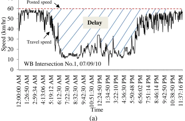
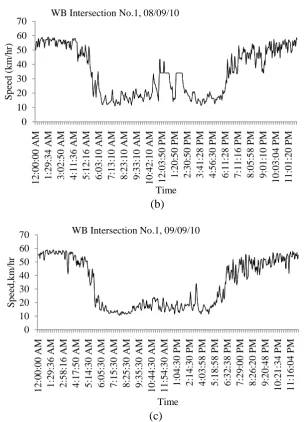
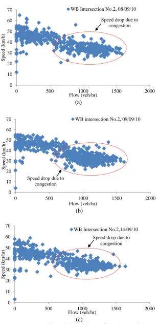
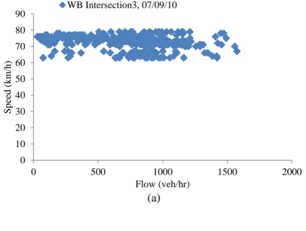
Figure 5.2 Speed-flow relationship for WB link of intersection 1 87 Figure 5.3 Speed variation for various survey days of STREAMS data 89 Figure 5.4 Speed-flow relationship for WB link at intersection 2 90 Figure 5.5 Speed variations for WB link at Intersection 2 92 Figure 5.6 Speed-flow relationship for WB link at intersection 3 93 Figure 5.7 Speed variations for the WB link at Intersection 3 94 Figure 5.8 Speed-flow relationships for the EB link at intersection 6 96 Figure 5.9 Speed variations for the EB link at Intersection 6 97 Figure 5.10 Speed-flow relationships for the EB link at intersection 5 98 Figure 5.11 Speed variations for the EB link at Intersection 5 100 Figure 5.12 Speed-flow relationships for the EB link at intersection 4 101 Figure 5.13 Speed variations for the EB link at Intersection 4 102 Figure 5.14 Speed-flow relationships for the EB link at intersection 3 104 Figure 5.15 Speed variations for the EB link at Intersection 3 105 Figure 5.16 Speed distributions in the WB and EB direction 106

Chapter 6 Figure title Page

(17)

xv

Figure 6.21 The efficiency of Scenario 2 in terms of traffic macroscopic aspect 128 Figure 6.22 The parameters of signalised intersection 2 before and after Scenario 3 130 Figure 6.23 The efficiency of Scenario 3 on the signalised parameters 132 Figure 6.24 The macroscopic characteristics before/after the application of

Scenario 3 133

Figure 6.25 The efficiency of Scenario 3 on the characteristics of congested link 134 Figure 6.26 Signalised intersection parameters under application of Scenario 4 136 Figure 6.27 The efficiency of Scenario 4 on the performance of intersection 2 138 Figure 6.28 The application of Scenario 4 on the link traffic characteristics 139 Figure 6.29 The efficiency of Scenario 4 on the link traffic parameters 141 Figure 6.30 Optimum efficiency of traffic scenarios regarding the intersection

characteristics 142

Figure 6.31 Annual delay time cost before and after applying VSL scenarios 143 Figure 6.32 Optimum efficiency of traffic scenarios regarding the link

characteristics 144

Figure 6.33 Annual vehicle accessibility after applying VSL scenarios 145 Figure 6.34 TTT comparison under control/non-control condition 145

Chapter 7 Figure title Page

Figure 7.1 Flow chart for traffic Scenario 1 (ITCS1) 150 Figure 7.2 Flow chart for traffic Scenario 2 (ITCS2) 151 Figure 7.3 Average queue length before and after applying ITCS1, SCL (a) 152 Figure 7.4 Average queue length before and after applying ITCS1, SCL (b) 153 Figure 7.5 Efficiency of ITCS 1, SCL (a) on average queue length 154 Figure 7.6 Efficiency of ITCS 1, SCL (b) on average queue length 154 Figure 7.7 Average delay before and after applying ITCS 1, SCL (a) 155 Figure 7.8 Average delay before and after applying ITCS 1, SCL (b) 155 Figure 7.9 Efficiency of ITCS 1, SCL (a) on average delay 156 Figure 7.10 Efficiency of ITCS 1, SCL (b) on average delay 156 Figure 7.11 Average stopped delay before and after applying Scenario1, SCL (a) 157 Figure 7.12 Average stopped delay before and after applying ITCS 1, SCL (b) 158 Figure 7.13 Efficiency of ITCS 1, SCL (a) on average stopped delay 158 Figure 7.14 Efficiency of ITCS 1, SCL (b) on average stopped delay 159 Figure 7.15 Average number of stops before and after applying Scenario1, SCL (a) 159 Figure 7.16 Average number of stops before and after applying Scenario1, SCL

(b) 160

(18)

xvi

Figure 7.36 Efficiency of ITCS 2, SCL (b) on average queue 172 Figure 7.37 Average delay before and after applying ITCS 2, SCL (a) 172 Figure 7.38 Average delay before and after applying ITCS 2, SCL (b) 173 Figure 7.39 Efficiency of ITCS 2, SCL (a) on average delay 173 Figure 7.40 Efficiency of ITCS 2, SCL (b) on average delay 174 Figure 7.41 Average stopped delay before and after applying ITCS 2, SCL (a) 175 Figure 7.42 Average stopped delay before and after applying ITCS 2, SCL (b) 176 Figure 7.43 Efficiency of ITCS 2, SCL (a) on average stopped delay 176 Figure 7.44 Efficiency of ITCS 2, SCL (b) on average stopped delay 177 Figure 7.45 Average number of stops before and after applying ITCS 2, SCL (a) 177 Figure 7.46 Average number of stops before and after applying ITCS 2, SCL (b) 178 Figure 7.47 Efficiency of ITCS 2, SCL (a) on average number of stops 178 Figure 7.48 Efficiency of ITCS 2, SCL (b) on average number of stops 179 Figure 7.49 Average speed before and after applying ITCS 2, SCL (a) 180 Figure 7.50 Average speed before and after applying ITCS 2, SCL (b) 180 Figure 7.51 Efficiency of ITCS 2, SCL (a) on average speed 181 Figure 7.52 Efficiency of ITCS 2, SCL (b) on average speed 181 Figure 7.53 Average flow before and after applying ITCS 2, SCL (a) 183 Figure 7.54 Average flow before and after applying ITCS 2, SCL (b) 184 Figure 7.55 Efficiency of ITCS 2, SCL (a) on average flow 184 Figure 7.56 Efficiency of ITCS 2, SCL (b) on average flow 185 Figure 7.57 Average density before and after applying ITCS 2, SCL (a) 185 Figure 7.58 Average density before and after applying ITCS 2, SCL (b) 186 Figure 7.59 Efficiency of ITCS 2, SCL (a) on average density 186 Figure 7.60 Efficiency of ITCS 2, SCL (b) on average density 187 Figure 7.61 Optimum efficiency of various traffic scenarios 188 Figure 7.62 Maximum improvement at the approach link of intersection 2 190 Figure 7.63 Comparison between traffic base and ITCS scenarios regarding TTT 191 Figure 7.64 Maximum efficiency of ITCS regarding TTT 192

Appendix A Figure title Page

Figure A.1 VISSIM background image of the study area 209 Figure A.2 Signal control window for intersection 1 211 Figure A.3 VISSIM snapshot for such vehicle type 212 Figure A.4 Acceleration and deceleration functions 212

Figure A.5 Static routes distributions 213

Figure A.6 Links behaviour 215

Figure A.7 Calibration Process 219

Appendix B Figure title Page

Figure B.1 Locations of controlled speed towards the EB direction 225 Figure B.2 The simulation of scenario 1 before and after VSL application 228 Figure B.3 The efficiency of scenario 1 on the signalised intersection

characteristics 230

(19)

xvii

Figure B.15 The efficiency of Scenario 4 in terms of intersection parameters 248 Figure B.16 The influence of Scenario 4 on speed, flow, and density 250 Figure B.17 The efficiency of Scenario 4 on the intersection properties 251 Figure B.18 Optimum efficiency in term of the intersection characteristics 252 Figure B.19 Optimum efficiency in term of the link characteristics 252

Figure B.20 TTT comparison 253

Figure B.21 The efficiency of VSL application on the TTT 253

List of Tables

Chapter 2 Table title Page

Table 2.1 Motor vehicle LOS thresholds at signalized intersections 10

Chapter 3 Table title Page

Table 3.1 Intersection names 44

Table 3.2 Number of lanes 44

Table 3.3 ADT for two weeks survey 46

Table 3.4 Speed and flow normalisation values 49

Table 3.5 Video camera locations and manual traffic recording 51 Table 3.6 Signal timing plan of the selected area 64

Table 3.7 Travel time field data for EB 66

Table 3.8 Travel time data for WB 66

Table 3.9 Optimum signal offsets 67

Chapter 4 Table title Page

Table 4.1 Total simulated traffic volume (veh/h) for the EB direction 74 Table 4.2 Total simulated traffic volume (veh/h) for the WB direction 74 Table 4.3 Estimation of minimum required number of simulation runs for EB 75 Table 4.4 Estimation of minimum required number of simulation runs for WB 75 Table 4.5 Calibrating simulated flow versus field observed flow for Beatty EB 77 Table 4.6 Calibrating the simulated flow versus field observed flow for Beatty

NB 77

Table 4.7 Calibrating the simulated flow versus field observed flow for Mains

EB 78

Table 4.8 Statistic validation for VISSIM modelling 81 Table 4.9 Comparison of simulated capacity and field capacity 83

Chapter 6 Table title Page

Table 6.1 Identification of controlled speed for WB 108

Table 6.2 Control speed activation system 108

Table 6.3 VSLs Scenarios 109

Table 6.4 Annual time savings from Scenario 1 113

Table 6.5 Delay statistical descriptive 114

Table 6.6 Delay, One-Way ANOVA 114

Table 6.7 Probability of fatality at GAR before and after utilising VSL 120 Table 6.8 Speed statistical descriptive for part 1 120

Table 6.9 Speed, One-Way ANOVA for part 1 120

Table 6.10 Speed statistical descriptive for part 2 121

(20)

xviii

Table 6.16 TTT cost after applying VSL 146

Chapter 7 Table title Page

Table 7.1 Annual delay time savings after using ITCS1 156

Table 7.3 Delay, One Way-ANOVA 157

Table 7.4 Maximum efficiency of ITCS 1 regarding intersection parameters 161 Table 7.5 Probability of fatality before and after using ITCS1 164 Table 7.6 Total annual savings in crash costs at GAR after applying ITCS1 164 Table 7.7 Speed statistical descriptive for part 1 164

Table 7.11 Maximum efficiency of ITCS 1 regarding link parameters 169 Table 7.12 Annual delay time savings cost after applying ITCS2, SCL (a) 174

Table 7.14 Delay, One-Way ANOVA 175

Table 7.15 Maximum efficiency of ITCS 2 for intersection parameters 179 Table 7.16 Probability of fatality at GAR before and after using ITCS2 181 Table 7.17 Total annual savings in crash costs a GAR after applying ITCS2 182 Table 7.18 Speed statistical descriptive for part 1 182

Table 7.22 Maximum efficiency of ITCS 2 regarding link parameters 187 Table 7.23 Maximum improvement due to VSL application and ITCS 188 Table 7.24 The annual savings in delay time for VSL and ITCS 189 Table 7.25 Maximum improvement regarding link parameters 189 Table 7.26 Maximum expected annual saving from VSL and ITCS application 190 Table 7.27 Total annual savings in crashes for BMA 190 Table 7.28 Maximum expected annual saving in TTT along GAR 191

Table 7.29 Total annual savings in TTT for BMA 192

Appendix A Table title Page

Table A.1 Modified look back distances for EB direction 216 Table A.2 Total simulated traffic volume for the EB lanes (veh/h) 222 Table A.3 Total simulated traffic volume for the WB lanes (veh/h) 222 Table A.4 Estimation of minimum required number of simulation runs for EB 223 Table A.5 Estimation of minimum required number of simulation runs for WB 224

Appendix B Table title Page

Table B.1 Identification of controlled speed for the EB lane 225

Table B.2 Speed control activation system 226

(21)

xix ABS Australian Bureau of Statistics

AD Australian Dollar

AIMSUN Advanced Interactive Microscopic Simulation for Urban and Non-urban Networks

ALINEA Asservissement Lineaire d’Entree Autoroutiere

AMOC Advanced Motorway Optimal Control

ARE Absolute Relative Error

ATC Area Traffic Control

BMA Brisbane Metropolitan Area

BTRE Bureau of Transport and Regional Economics CORSIM CORridor SIMulation

DTMR Department of Transport and Main Roads EMME Equilibre Multimodal, Multimodal Equilibrium

EP Evening Period

FMS Freeway Management Systems

GAR Griffith Arterial Road

GEH Geoffrey E. Havers

HCM Highway capacity manual

HDC High Definition Cameras

HV Heavy Vehicle

ITCS Integrated traffic control system

LOS Level of Service

METANET Modèle d’Ecoulement du Trafic Autoroutier: NETwork

MFD Macroscopic Fundamental Diagram

MOE Measures of Effectiveness

MP Morning Period

MPC Model Predictive Control

MTFC Mainstream Traffic Flow Control PARAMICS PARAllel MICroscopic Simulation

QDTMR Queensland Department of Transport and Main Roads QDTMR

QLD Queensland

RLC Red-Light Camera

RLR Red-Light Running

SATURN Simulation and Assignment of Traffic to Urban Road Networks

SCL Speed Control Limit

STREAMS Synergised Transport Resources Ensuring an Advance Management System

TDM Travel Demand Management

TFL Transport for London

TH, RT, LT Through, Right turn, Left turn TRANSYT TRAffic Network StudY Tool

TRB Transportation Research Board

TTT Total Travel Time

TU, WE, THU Tuesday, Wednesday, Thursday VISSIM Verkehr In Städten-SIMulationsmodel

VMS Variable Message Sign

VSL Variable Speed Limit

(22)

(23)

1

CHAPTER ONE

Introduction

Background

1.1

Road traffic congestion is considered one of the most significant transportation problems throughout the world due to its impact on both the environment and economy. It typically occurs when traffic demand is close to or exceeds the available volume capacity of the road network. Solving traffic congestion is complex as traffic demand is not constant but varies according to season, day of the week, and the time of day. In addition, capacity is not constant, as it can reduce due to inclement weather, the presence of work zones, traffic incidents or other events. Increasing the demand or decreasing the capacity of a road system may lead to problems for both vehicle users and society. This congestion phenomenon commonly emerges in major cities on heavily trafficked roads. Congestion has a negative impact on the efficiency of the traffic system, safety, the environment (air contamination, fuel consumption), and the quality of life (health problems, noise, frustration), (Bellemans et al., 2006, Hongfeng et al., 2008).

Metropolitan vehicle travel in Australia is expected to continue to grow appreciably over the next decade and a half. Australian Bureau of Statistics (ABS) (2013) estimated there were 16.6 million vehicles registered in Australia in 2012 and that passenger vehicles made up 76.4% of all registered vehicles. Motor vehicles registered in Australia travelled an average of 14,000 kilometres per vehicle in 2012. Bureau of Transport and Regional Economics (BTRE) ( 2007) estimated that in 2005 the total social costs of congestion in Australian capital cities was $9.4 billion. This total was comprised of approximately $3.5 billion in private time (losses from trip delay and travel time variability), $3.6 billion in business time costs (trip delay plus variability), $1.2 billion in extra vehicle operating, and $1.1 billion in extra air pollution damage costs. In the absence of improved congestion management, BTRE (2007) estimated that the social costs of congestion would be increased to $20.4 billion by 2020.

This thesis investigates the possibility of using variable speed limits (VSLs) for control of upstream traffic as a proposed traffic control strategy on the Griffith Arterial Road (GAR) in Brisbane (Figure 3.2). The research investigates the contribution of VSL to managing and operating existing transportation infrastructure for the purpose of increasing efficiency, safety, and mobility, and improving the environment by minimising delay, queue length, and number of stops, and increasing flow and speed.

Objectives of the study

1.2

The aim of the research was to investigate how dynamic variable speed limits (VSL) and signal control systems could be used in an integrated approach to traffic management to improve the traffic efficiency, safety, and mobility of a congested urban road network.

(24)

2

strategies. Selecting the optimum traffic management strategies was based on the consideration of several key parameters such as average delay, average stopped delay, average queue, and number of stops.

Using the GAR as a case study, the main components of the research are:

1. To evaluate the real traffic behaviour on an urban arterial road, and develop a VISSIM (Verkehr in Städten-Simulations) model based on data collected from real traffic,

2. To investigate the effect of using VSL controls on the level of service (LOS) at critical signalized intersections,

3. To explore the effect of using VSL controls on the performance of congested arterial roads in terms of speed, flow, and density,

4. To investigate the influence of VSL controls on the traffic safety during the congestion period,

5. To investigate the potential of integrating VSL control with other traffic congestion management (increase the signal timings of critical intersection), and 6. To optimise and identify the appropriate traffic control using VSL and Integrated

traffic control system (ITCS).

Significance of the study

1.3

There are many definitions of an integrated traffic management system but in general, they refer to the use of distributed computer architecture where intersection control is utilised to optimise flow through an adaptive system.

This research moves to the next level through the application of VSL integrated with an existing signalised intersection control within a link. This is depicted schematically in Figure ‎1.1.

Most past research has been focused on using VSL applications on motorways for improving the traffic efficiency and safety. Exploring the effectiveness of VSL control on a signalised arterial road network has the potential to provide a new traffic management technique for busy arterial roads. It is considered that the main benefits of applying VSL to an urban arterial road will be to:

1. Enhance the performance of existing transportation infrastructure and reduce the need to construct new roads or add lanes,

2. Provide cost effective options to the mobility problems by low-cost solutions, 3. Improve the traffic efficiency, safety , and mobility for urban arterial roads, and 4. Provide an environmental friendly approach to reduce vehicle total travel time

(25)

3

Figure ‎1.1 Schematic illustration showing the scope of the current research

Study methodology

1.4

The study methodology adopted may be depicted schematically as shown in Figure ‎1.2.

Introduction _{Research gap}

Review TDM strategies and the performance of VSL on motorway regarding traffic efficiency and safety

Investigation the efficiency of VSL on urban arterial road

Collecting traffic data for selected urban arterial road

Field survey Road authority

Building VISSIM platform

Model calibration using real traffic data Model validation (GEH)

Replication the actual traffic behaviour for selected urban arterial road

Investigation the effect of VSL as a single application

Signalised intersection features Delay, Queue, Stops

Arterial Link performance Speed, Flow, Density

Investigation the effect of integrating VSL & traffic control congestion

(ITCS)

(26)

4

Figure ‎1.2 Study methodology

Thesis layout

1.5

The thesis is presented in a series of integrated chapters. Chapter two reviews traffic control management strategies used to alleviate or mitigate traffic congestion in urban areas and explore the effect of an Intelligent Transport System (ITS) on traffic performance of an interrupted flow. Chapter three provides details of the methods that were used to collect field data. It also provides the reasons for selecting the Griffith Arterial Road (GAR) in Brisbane as the case study area for the present research. Chapter four provides an overview of VISSIM software, its use in traffic modelling and describes the process of calibration and validation of the software. Chapter five describes the local traffic situation for GAR under base line conditions. Chapter six investigates the effect of using (only) VSL control on the performance of GAR. Chapter seven investigates the improved efficiency obtained by integrating VSL control with changes in the signal timings of congested intersections. Chapter eight presents the conclusions and discusses possible extensions of the research.

1 • Reconnaissance

2 • Selection of study area

3 • Pilot survey

4 • Data collection

5 • VISSIM modelling

6 • Analysis of existing traffic conditions

7 • Evaluation of using VSL

8 • Optimisation of VSL scenarios

9

• Evaluation of integrating VSL application with other congestion management tools

10 • Selection of optimal traffic operation

(27)

5

2

CHAPTER TWO

Literature Review

Introduction

2.1

Various traffic management strategies are frequently applied to deal with traffic in busy arterial roads in urban areas. Despite these efforts, traffic congestion continues to increase on arterial roads, particularly during peak periods. Traffic bottlenecks at intersections are the main cause of congestion. Traffic congestion is a source of immobility and efficiency loss, safety reduction, fuel consumption, excessive air pollution, health problems, noise and frustration.

A number of traffic management strategies have been proposed for alleviating cities’ traffic congestions such as diverting traffic from peak-period to off-peak period, using congestion pricing, constraint flow, reducing speed limits, coordinating traffic lights along major arterials, actuated traffic signals, and adding additional lanes where expanding the road network is feasible.

As a result of the continuous increase of traffic in central urban areas, traffic congestion and delays are often experienced in the vicinity of intersections. This negatively affects the arterial road network (Garber and Hoel, 2009). Under non- saturated flow conditions (normal), traffic signals are designed to provide safe and efficient traffic operation by reducing vehicle delays and the number of stops. By contrast, in congested conditions, traffic queues and delays propagate from cycle to cycle either due to insufficient green signal time allocations or because of blockages. Excessive queues and spillbacks towards upstream flow may lead to gridlock in the network resulting in serious degradation of the traffic system.

(28)

6

Variable speed limits are commonly used to regulate traffic flow on motorways by using variable speed message signs (VSMs). The original aim of VSMs was to improve traffic safety by increasing driver compliance. This led to decreasing rear-end collisions as reported by Zackor (1979) and Coleman et al. (1996). Smulders (1992) and Harbord (1995) investigated the use of speed limits and explained how speed limits had a homogenising effect on traffic flow during the peak periods. Chien et al. (1997) and Lenz et al. (2001) focused on how variable speed limits could reduce inbound traffic at bottlenecks, which avoided or alleviated traffic congestion. Kohler (1974) found that when the headways in a chain of vehicles were below a specific threshold, the chain became unstable.

Inhomogeneity in traffic flow can contribute to small perturbations in the flow which might then cause congestion to occur. Inhomogeneity in traffic can arise due to variations in speed between consecutive vehicles in one lane or different lanes, or flow differences among the lanes.

VSL strategies can create a more uniform distribution of traffic density over freeway links preventing the high traffic density that leads to breakdowns in traffic flow. Alessandri et al. (2002) reported that VSL controls were able to prevent congestion and improve flow using segment throughput as a measure of effectiveness, but that it had little impact on the reduction of total travel time (TTT) in the network. Hegyi et al. (2005) evaluated the impact of using VSL controls on the total travel time (TTT) as a measure of effectiveness using a hypothetical network. Their results showed a 21% saving in TTT could be achieved when using a VSL control strategy. Kejun et al. (2008) investigated the effect of VSL on a hypothetical 5 km work zone model. The study did not find any significant improvement in TTT. Lee et al. (2006) reported that VSL controls used in highly congested locations, reduced the potential for crashes and increased the safety by 25%, but that they also increased TTT. This finding was supported by Allaby et al. (2007). In contrast, Abdel-Aty et al. (2008) found that VSLs achieved a significant reduction in crash potential during non-congested periods, but had no significant influence during the non-congested periods. VSL controls are widely used in European countries and the United States. The key difference in the use of VSLs in those areas is enforcement, where within Europe automated speed enforcement was used to achieve high driver compliance rates in European countries. For example, Transport For London (TFL) (2004) reported a 9% reduction in flow breakdown (escalating vehicles speed) and a 6% reduction in stop-go driving conditions (reducing number of vehicle stops). The VSL applications resulted in traffic headways becoming more uniformly distributed within the narrow range of 0.8-1.5 seconds.

(29)

7

congestion. Specifically, they found improvements in total travel time, total travel distance, and total flow around 39%, 8%, and 5.5%, respectively.

In summary, inconsistent outcomes have been achieved by the application of VSL. It should be noted that, almost all VSL evaluation studies have been concentrated on a small number of links in the corridor. Moreover, those studies do not take into consideration the effect of speed limit on the non-congested links in the evaluation process. Most previous studies indicated that VSL applications were capable of improving the travel time, but that it had little impact on the flow. The studies have also showed consistent safety improvement by reducing speed variance or improving speed homogenization.

This chapter presents a review of the important measures used to characterise the operational quality of signalised intersections in terms of delay, queue length and number of vehicle stops. It also presents a brief description of some of the traffic control management strategies used to improve the performance of traffic flow in urban cities. Given the importance of VSL in the research, the theory underpinning the application of VSL in an interrupted flow condition is outlined.

The performance of signalised intersections

2.2

Traffic signals at intersections represent point (node) locations within urban arterial road networks. At these point locations, the measures of operational quality or effectiveness based on traffic speed and density are not relevant. Speed has no meaning at a point, and density requires a section of some length for measurement. The three measures of effectiveness commonly used to characterise the operational quality of signalized intersections are delay, queue length, and number of stops. The most common parameter used to describe traffic performance at a signalised intersection is delay, with queue length and/or number of stops often used as a secondary measure (Roess et al., 2004).

Delay 2.2.1

Delay at signalized intersections is associated with the time lost to a vehicle and/or driver due to the presence of traffic signals, geometric design of the road and traffic conditions (Darma et al., 2005). Delay is also defined as the difference in travel time between when a vehicle is affected and unaffected by a controlled intersection under ideal conditions. Ideal condition is when there is an absence of geometric delay, no incidents, and when there are no other vehicles on the road Transportation Research Board (TRB) (2000).

(30)

8

(Teply et al., 1995). While stopped delay is easier to measure, overall delay (control delay) provides a better measure of the operational quality of a signalised intersection. The delay caused by a decelerating or accelerating vehicle is categorized as deceleration or acceleration delay. Several delay types used in the HCM at a signalized intersection for a single vehicle approaching a red signal are shown in Figure ‎2.1, (TRB, 2000).

Figure ‎2.1Delay components, Source: (TRB, 2000)

In the figure, stopped delay for the vehicle includes only the time spent stopped at the signal. It starts when the vehicle is fully immobilised and terminates when the vehicle starts to accelerate. Approach delay comprises an additional lost time due to the deceleration and acceleration. It is set up by extending the speed slope of the approaching vehicle as if no signal existed and the departure slope after full speed is achieved. Then the approach delay is the horizontal (time) difference between the hypothetical and departure speed slope. Time in queue delay cannot be effectively shown using one vehicle because it involves joining and departing a queue of several vehicles.

In TRB (2000), the average delay per vehicle for a lane group is computed as follow:

2.1

with

( )

[ ( ) ] 2.2

[( ) √( ) ] 2.3

( ) 2.4

where,

d = average overall delay per vehicle (seconds/vehicles),

Vehicle trajectory with stop

1 2

4

3

D

ist

an

ce

Time

1 Stopped delay 2 Deceleration delay 3 Acceleration delay 4 Approach delay 5 Control delay Vehicle trajectory without stop

(31)

9

d1 = uniform delay (seconds/vehicles),

d2 = incremental, or random, delay (seconds/vehicles),

d3 = residual demand delay to account for over-saturation queues that may

have existed before the analysis period (seconds/vehicles),

PF = adjustment factor for the effect of the quality of progression in coordinated systems,

C = traffic signal cycle time (seconds),

g = effective green time for lane group (seconds),

X = volume to capacity ratio of lane group,

c = capacity of lane group (vehicles/hour),

k = incremental delay factor dependent on signal controller setting (0.50 for pretimed signals; vary between 0.04 to 0.50 for actuated controllers),

I = upstream filtering/metering adjustment factor (1.0 for an isolated intersection),

T = evaluation time (hours),

P = proportion of vehicles arriving during the green interval,

fp = progression adjustment factor.

In this delay model the residual delay components d3make use of vehicles instead of

passenger car units to quantify traffic flows. The period analysis T is reported in hours instead of minutes, but this change is reflected in the use of a different multiplication factor in each term involving the variable T. In Equation 2.3, parameters k and I are introduced in the last term of the equation, and this term reduces to 0.5 and 1.0 when the values associated with pre-timed traffic signal control and an isolated intersection respectively.

Based on the delay formula in TRB (2000), VISSIM software is used to compute the total delay every deci-second for every vehicle completing the travel time section by subtracting the theoretical (ideal) travel time from the real travel time. The theoretical travel time is the time that would be reached if there were no other vehicles and no signal controls or other stops in the network. The total delay is computed as the summation of all instantaneous delays along a link, for an entire trip, and for an entire network, (Van Aerde and Rakha, 2007).

∑ ∑[ ( )] 2.5 where,

D = the total delay incurred over entire trip,

di = the delay incurred during interval i,

Δt = the duration of interval,

u(t+iΔt) = the vehicle instantaneous speed in interval i,

uf = the expected free-flow speed of the facility on which the vehicle is

traveling, and N = the number of time intervals in a speed profile.

(32)

10

to maintain stability. Secondly, incident delay may cause an additional time lose due to an incident condition. Thirdly, traffic delay may be caused by the interaction of vehicles, as a result of drivers having to reduce their speed below the free flow speed due to traffic conditions. Total delay of a vehicle is the sum of control, geometric, incident, and traffic delay. Driver perception and reaction time variations to the changes of traffic signal display at the start of green interval and during yellow interval to mechanical constraints and to individual driver behaviour also contribute to the traffic delay at signalized intersection. Most delay incurred at signalised intersections is due to the traffic signal operation itself while only a fraction of the entire delay is attributed to the time required by the driver to react to the traffic signal changes which depends on the driver behaviour.

Average control delay is used as the basis for determining the level of service (LOS) for a signalised intersection (TRB, 2000). Delay minimization is frequently used as a primary optimization criterion when determining the operating parameters of traffic signals at both isolated and coordinated signalized intersections. Intersection control delay is generally computed as a weighted average of the average control delay for all lane groups based on the volume within each lane group. Caution should be exercised when evaluating an intersection based on a single value of control delay because this is likely to over represent or under-represent operations for individual lane groups. Table ‎2.1 (TRB, 2000) provides the criteria of LOS levels for a signalised intersection. Six levels of service are assigned the letters A through F. Each LOS represents a range of operating conditions, with LOS A representing the best operating conditions and LOS F the worst. A higher delay experienced by vehicles at signalised intersection is represented by a low LOS.

Table ‎2.1 Motor vehicle LOS thresholds at signalized intersections

LOS Control Delay per vehicle

(seconds per vehicle)

A ≤‎10

B > 10-20

C > 20-35

D > 35-55

E > 55-80

F > 80

Source: (TRB, 2010)

Vehicle queuing 2.2.2

(33)

11

Deterministic queuing analysis is one of the most commonly utilized approaches for estimating queue lengths at the macroscopic level because it is relatively simple. In this analysis, vehicles are assumed to queue vertically at the intersection stop line for under-saturated and oversaturated conditions. When traffic demand is under saturated, the estimates of maximum queue length at signalized intersections can be computed using the following equation (TRB, 2000).

2.6

where,

r = red interval (seconds),

s = saturation flow rate (vehicles/second),

q = arrival flow rate (vehicles/second).

Alternatively, when traffic demand is oversaturated, a residual queue remains at the end of the green interval. The difference between the arrival flow rate and the capacity of a signalized intersection gives the residual queue of vehicles at the end of a cycle. When the residual vehicles of a first cycle are known, the residual vehicles of the last cycle can be determined as the residual vehicles of the first cycle multiplied by the number of cycles (N). From the residual queue length at the end of each cycle an approximate estimate of the maximum queue length for each cycle at an oversaturated fixed-time signalized approach is calculated as indicated in the following equations (TRB, 2000).

[ ( ) ] 2.7 [( )( ) ] 2.8

where,

Qres = residual queue length of end of each cycle (vehicles),

N = number of cycle,

q = arrival flow rate (vehicles/second),

g = green interval (seconds),

s = saturation flow rate (vehicles/second), and

Qmax = approximate estimate of maximum queue length during a cycle

(vehicles).

Shock wave theory can also be used to estimate queue lengths at signalized intersections. The main difference between shock wave and queuing analysis models is in the way vehicles are assumed to queue at the intersection stop line. Shock wave considers that vehicles are queued horizontally one behind each other. This means that each vehicle occupies a physical space and allows the analysis to capture more realistic queuing behaviour and to more realistically compute the extent of the queue. The maximum extent of queue and maximum number of queued vehicles caused by the fixed-time signalized intersection is shown as following respectively (TRB, 2000).

₍ _{) (} ₎ 2.9

2.10 where,

q = arrival rate (vehicles/second),

(34)

12

kd = density of discharge flow (vehicles/kilometre),

kj = jam density (vehicles/kilometre),

ka = density of approach flow (vehicles/kilometre),

xm= distance of maximum extent queue (kilometres), and

NQ = number of vehicles in maximum queue (vehicles).

In the case of the VISSIM software, the user defines a queue according to the maximum vehicle speed for the beginning of the queue (default is 5 km/hr), the minimum vehicle speed at its end (default is 10 km/hr), and the maximum spacing between vehicles (default is 20 metres). It allows the user to identify a queue counter location. The distance to the farthest upstream point of any queue at this location is calculated. If the queue backs up onto multiple links, the longest distance is recorded. If the front of the queue begins to discharge, VISSIM keeps tracking to the back of the queue until no queued vehicles remain between the queue counter location and the current back of queue (Dowling, 2007). It is not the average of the back of queues when the signals turn from red to green that is calculated but the average queue of each time step, irrespective of signal head colour as indicated in the following equation.

∑ ( ) 2.11

where,

Qavg= average back of queue over analysis period (meters),

Q(i) = observed back of queue length (meters) at end of time step (i) and

I = total number of time steps in analysis period.

Approaches to signals that experience extensive queues are likely to also experience more rear-end collisions (Rodegerdts et al., 2004). Wiles et al. (2005) stated that queue growth for a particular intersection is more likely to affect arrival drivers than departing drivers. Additionally, in many instances, multiple lanes were found to be impacted due to driver behaviour seeking access to network. Although urban drivers are generally aware of traffic conditions that are likely to be encountered in their daily travels, they still can be surprised by abrupt and extensive queues. Drivers unfamiliar with conditions might not be alert and be involved with or cause collisions. All drivers are particularly vulnerable when poor road geometric conditions coincide with queue build-up.

Yan et al. (2005) and Sugiyama and Nagatani (2012) indicated that rear-end crashes are the most common accident type at signalized intersections. These crashes result from a combination of lead-vehicle deceleration and inadequate deceleration by the following vehicle. Driving during the peak periods results in smaller headways between leading and following vehicles, which increases the possibility of rear-end crashes. Khattak (2001) reported that a majority of the crashes (54.9%) occurred during the peak hours of 7:00-9:00 a.m. and 3:00-6:00 p.m.

(35)

13

rear-end crashes. The estimated number of collisions at traffic signals was reduced by 9%. A strong relationship between increase in cycle length and reduction of vehicular conflicts was observed by the researchers.

Number of stops 2.2.3

The third important factor for evaluating the performance of traffic at signalised intersections is the number of vehicle stops in the road segment approaching the signalised intersection. This factor reflects how frequently drivers have to stop while traveling along a roadway because of traffic signals, turning vehicles, pedestrian area, and similar factors. Speed thresholds were often used to determine when a vehicle is stopped. The only non-arbitrary speed threshold for this purpose is zero. Practical considerations propose that simulation modelling that deals with stopping would be more stable if a near-zero speed were used instead. Some simulation modelling was applied (8 km/h) for determining number of stops when a vehicle has “stopped”.

The accumulation of multiple stops poses more problems and usually depends on random thresholds that vary among various intersection management tools. The major problem with multiple stops is that after the first stop, later stops occur from a lower speed and therefore have a less adverse influence on driver comfort, operating costs, and safety. The estimated number of vehicle stops is important in safety considerations, traffic operations, vehicle fuel consumption and emissions.

For signalised approaches, some models use the probability of stopping where the maximum probability is 100% which means that the maximum number of stops is 1.0 on any approach. In other modelling algorithms subsequent stops are based on the release from the stopped state when the vehicle reaches an arbitrary threshold speed, often around 24 km/hr (TRB, 2010). Deterministic and simulation models are common tools for estimating the number of stops, and most allow user-specified values for the parameters that establish the start and end of a stop.

Many researchers (Webster, 1958); (Catling, 1977); (Cronje, 1983) have established definitions to deal with this measure of performance. An important contribution was by Webster (1958) who generated stop and delay relationships by simulating a one-lane approach at an isolated signalized intersection. In particular, simulation results have been a fundamental concept to developing traffic signal operating procedures since the concept was first generated. The number of vehicle stops using queuing analysis is computed as all vehicle arrivals when the traffic signal is red or when a queue exists at the approach stop line. The number of stops per vehicle can be calculated using the following equation.

( ) 2.12

where,

Ns = number of stops per vehicle (stops/vehicle),

s = saturation flow rate (vehicles/second),

C = cycle length (seconds),

q = arrival flow rate (vehicles/seconds),

r = red interval (seconds).

(36)

14

be derived with the assumption of a random arrival pattern as indicated in the following equation.

( )

[ ( )]

2.13

where,

Ns = number of passenger car units stopped at least once during the

evaluation time,

kf = adjustment factor for the effect of the quality of progression from delay

formula,

q = arrival flow (passenger car unit/hour),

ge = effective green interval (seconds),

C = cycle length (seconds),

y = lane flow ratio; y = q / S capped at y ≤ 0.99, with

S = saturation flow (passenger car unit/hour),

te = evaluation time (minutes).

The formula was developed further for estimating the number of vehicle stops under saturated conditions by Catling (1977) and Cronje (1983).

Catling (1977) used classical queuing theory to imitate oversaturated traffic conditions and developed an estimation method for a full queue length that captured the time-dependent nature of queues.

Cronje (1983) developed equations for estimating the queue length and number of stops under a fixed-time signal operation. The models developed by Catling and Cronje were used for both under and over-saturated traffic conditions.

[( _{( )}) ] 2.14 where,

N = number of stops per cycle (stops/cycle),

q = average arrival rate (vehicles per second),

s = saturation flow rate (vehicles per second),

r = effective red interval (second),

( )

( ) 2.15

I = ratio of variance to the average of the arrivals per cycle, = 1 for Poisson distribution,

( ) ( )_2.16

( )( ) _2.17

g= effective red interval (second),

x = v/c ratio; degree of saturation,

v = traffic volume (veh/hr), and

c = road capacity (veh/hr).

(37)

15

∑ ( ) ( )

( ) ( ) 2.18

where,

S = estimated partial stops,

ui , ui-1 = speed of vehicle at time i and time i-1 (kilometres/hour),

uf = free speed on travelled link (kilometres/hour).

VISSIM computes a vehicle stop when a vehicle changes its speed from any speed greater than 0 to a speed of 0, that is when a vehicle comes to a standstill. The approach does not account for partial stops. VISSIM also reports the number of stops within the queue, which are defined as events when the vehicle enters the queue, that is when its speed falls below the speed for the beginning of the queue (PTV, 2011). Reducing the value of this measure of effectiveness reflects a significant increase in efficiency of traffic flow and safety along an urban arterial road (Zhou et al., 2013); (Factor et al., 2012); (He and Hou, 2012).

Traffic control management strategies

2.3

Many travel demand management (TDM) strategies to suppress traffic congestion in cities have been proposed in the literature. The following sections present a brief description of some of the strategies that have a large effect on traffic flow performance in cities.

Road pricing strategies 2.3.1

Road pricing strategies have been implemented in many countries to reduce traffic congestion. The objective of such a strategy is to alter the travellers’ behaviour, to reduce congestion by charging them an amount of money for using a network during specific periods (for example during “rush” hours). There are three main model categories: Marginal-Cost Pricing Models, Bottleneck Models, and Cordon Models. The theoretical background of the Marginal-Cost Pricing Model relies on all links being tolled. Initial work was reported by Pigou (1912), Vickrey (1963), and later by Beckmann (1967). If the charge postulated on each link in the network equals the additional congestion cost on other car users, revenue is maximized. The Bottleneck Model, otherwise known as the second-best toll model, was studied by Marchand (1968) using a general equilibrium model for two routes where an untolled alternative road was available parallel to a toll road in the network for a fixed time period. The second-best pricing models are described in Arnott et al. (1990) and McDonald (1995), where bottleneck tolls are charged on selected roads.

(38)

16

downtown areas. Hongfeng et al. (2008) explained that Singapore has long experience in successfully implementing area tag licensing and roadway pricing schemes as one of its major strategies to deal with traffic congestion. The initial reduction in traffic flow entering the control area was 44% and declined further to 31% by 1988, despite an increase in employment of 30% and an increase in vehicle ownership of 77% during the same period. Zhang and Yang (2004) investigated cordon-based, second-best congestion pricing problems on road networks involving optimal selection of toll levels and toll locations. The study revealed that the elastic-demand traffic equilibrium constraint maximized social welfare. The same study explained the impact of implementing different pricing scenarios on trips for various lengths. Figure ‎2.2 shows the distribution of trip length for four cases: the marginal-cost or first-best pricing, the single-layered and double-layered cordon pricing and no toll pricing. The figure reflects the impacts of alternative pricing strategies on car users travelling between various origin-destinations pairs related to different trip lengths. Firstly, for trips of less than 10 min, there was an increase in demand after presenting cordon pricing compared with the no tolling case while the demand decreased respect to the marginal-cost pricing case. This was attributed by the researchers to a simple fact that drivers try to avoid toll charges when the distance of travel is short and do not cross over the toll cordon. Secondly, for trips between 10 and 35 min, the demand for no tolling charge increased rapidly in contrast with cordon pricing scheme. The demand for single cordon pricing is slightly higher than double- cordon pricing. This is because the cordon-based, second-best route primarily affects medium length trips and makes demand drop. Finally, for trips greater than 35 min, the demand after implementing the cordon-pricing plan decreased compared with no toll case whereas it is higher for marginal cost pricing. This reflects the fact that cordon pricing has limited effect on long distance travel demand.

Figure ‎2.2 Traffic entering the restricted zone under electronic road pricing Source: Zhang and Yang (2004)

(39)

17

ERP is implemented on the road network. Such a variable pricing scheme creates a good opportunity to investigate the relationship between issues relating to congestion pricing. Luk and Hepburn (1993) studied the relationship between the elasticity of traffic volume and ERP rates for different locations and time periods using the arc formula. Figure 2.3 illustrates the effect of ERP on inbound flow over a time interval. The formula is as follow:

( )

( ) 2.19

where,

Average traffic demand before and after the change and

Price before and after the change.

Figure ‎2.3 Traffic entering the restricted zone under ERP, (1998) Source:Olszewski and Xie (2005)

There are many reports on using congestion pricing as a strategy to mitigating congestion of cities. However, there are some negative attitudes exhibited by drivers regarding this method. Verhoef et al. (1997) and Jones (1995) identified the concern of drivers about penalties that how to pay for using urban roads. This study found that drivers regarded themselves as victims of congestion and felt that they were not responsible for it, and as such they should not have to pay for it. More details about driver attitudes towards pricing congestion are found in Jones et al. (1991). Hongfeng et al. (2008) investigated the public attitude towards policy instruments for congestion mitigation in Shanghai. The study revealed that users had a negative attitude towards traffic policies such as congestion pricing, higher parking charges in congested areas and car restrictions.

Constraint traffic flow strategy 2.3.2

(40)

18

metropolitan areas in developing countries. Wardrop (1953) studied the evolution of macroscopic models in arterial roads, and extended the concept to involve general road networks.

Smeed (1966) revealed that the maximum flow that could enter a city centre would be a function for that city. Vehicles per unit time per unit width of road are normally considered to represent the capacity of a road. Thomson (1967) pointed out that the relationship between average speed and flow appeared to be a linear-decreasing relationship (data collected refers to uncongested condition). This finding was based on data collected from streets in the metropolitan London over many years.

Zahavi (1972) postulated that traffic volume behaved inversely to speed of traffic. The study analysed the correlation between traffic volume and speed for different cities in Great Britain and the United States of America by augmenting data related to various regions of a city through the same time interval. This concept (Zahavi’s theory) applies when traffic volume is low as the model is unable to cope with overloaded traffic conditions if the volume is high. Therefore, these models are not suitable to depict the peak period in a traffic jam.

Herman and Prigogine (1979) established a two-fluid model which explained the macroscopic relations of vehicular traffic in megacities. The model proposed tha