Think DSP: Digital Signal Processing in Python

(1)

Think DSP

Digital Signal Processing in Python

(2)

(3)

Think DSP

Digital Signal Processing in Python

Version 1.0.5

Allen B. Downey

Green Tea Press

(4)

Green Tea Press 9 Washburn Ave Needham MA 02492

Permission is granted to copy, distribute, and/or modify this document under the terms of the Creative Commons Attribution-NonCommercial 3.0 Unported License, which is available athttp://creativecommons.org/

(5)

Preface

Signal processing is one of my favorite topics. It is useful in many areas of science and engineering, and if you understand the fundamental ideas, it provides insight into many things we see in the world, and especially the things we hear.

But unless you studied electrical or mechanical engineering, you probably haven’t had a chance to learn about signal processing. The problem is that most books (and the classes that use them) present the material bottom-up, starting with mathematical abstractions like phasors. And they tend to be theoretical, with few applications and little apparent relevance.

The premise of this book is that if you know how to program, you can use that skill to learn other things, and have fun doing it.

With a programming-based approach, I can present the most important ideas right away. By the end of the first chapter, you can analyze sound recordings and other signals, and generate new sounds. Each chapter intro-duces a new technique and an application you can apply to real signals. At each step you learn how to use a technique first, and then how it works. This approach is more practical and, I hope you’ll agree, more fun.

0.1

Who is this book for?

The examples and supporting code for this book are in Python. You should know core Python and you should be familiar with object-oriented features, at least using objects if not defining your own.

(6)

I use NumPy and SciPy extensively. If you are familiar with them already, that’s great, but I will also explain the functions and data structures I use. I assume that the reader knows basic mathematics, including complex num-bers. You don’t need much calculus; if you understand the concepts of inte-gration and differentiation, that will do. I use some linear algebra, but I will explain it as we go along.

0.2

Using the code

The code and sound samples used in this book are available fromhttps:

//github.com/AllenDowney/ThinkDSP. Git is a version control system that allows you to keep track of the files that make up a project. A collection of files under Git’s control is called a “repository”. GitHub is a hosting service that provides storage for Git repositories and a convenient web interface. The GitHub homepage for my repository provides several ways to work with the code:

• You can create a copy of my repository on GitHub by pressing theFork button. If you don’t already have a GitHub account, you’ll need to create one. After forking, you’ll have your own repository on GitHub that you can use to keep track of code you write while working on this book. Then you can clone the repo, which means that you copy the files to your computer.

• Or you could clone my repository. You don’t need a GitHub account to do this, but you won’t be able to write your changes back to GitHub.

• If you don’t want to use Git at all, you can download the files in a Zip file using the button in the lower-right corner of the GitHub page. All of the code is written to work in both Python 2 and Python 3 with no translation.

(7)

0.2. Using the code vii

• NumPy for basic numerical computation,http://www.numpy.org/; • SciPy for scientific computation,http://www.scipy.org/;

• matplotlib for visualization,http://matplotlib.org/.

Although these are commonly used packages, they are not included with all Python installations, and they can be hard to install in some environments. If you have trouble installing them, I recommend using Anaconda or one of the other Python distributions that include these packages.

Most exercises use Python scripts, but some also use Jupyter notebooks. If you have not used Jupyter before, you can read about it athttp://jupyter.

org.

There are three ways you can work with the Jupyter notebooks:

Run Jupyter on your computer If you installed Anaconda, you probably got Jupyter by default. To check, start the server from the command line, like this:

$ jupyter notebook

If it’s not installed, you can install it in Anaconda like this

$ conda install jupyter

When you start the server, it should launch your default web browser or create a new tab in an open browser window.

Run Jupyter on Binder Binder is a service that runs Jupyter in a vir-tual machine. If you follow this link, http://mybinder.org/repo/

AllenDowney/ThinkDSP, you should get a Jupyter home page with the notebooks for this book and the supporting data and scripts.

You can run the scripts and modify them to run your own code, but the virtual machine you run in is temporary. Any changes you make will disappear, along with the virtual machine, if you leave it idle for more than about an hour.

View notebooks on nbviewer When we refer to notebooks later in the book, we will provide links to nbviewer, which provides a static view of the code and results. You can use these links to read the notebooks and listen to the examples, but you won’t be able to modify or run the code, or use the interactive widgets.

(8)

Contributor List

If you have a suggestion or correction, please send email to

[email protected]. If I make a change based on your feed-back, I will add you to the contributor list (unless you ask to be omitted).

If you include at least part of the sentence the error appears in, that makes it easy for me to search. Page and section numbers are fine, too, but not as easy to work with. Thanks!

• Before I started writing, my thoughts about this book benefited from con-versations with Boulos Harb at Google and Aurelio Ramos, formerly at Har-monix Music Systems.

• During the Fall 2013 semester, Nathan Lintz and Ian Daniher worked with me on an independent study project and helped me with the first draft of this book.

• On Reddit’s DSP forum, the anonymous user RamjetSoundwave helped me fix a problem with my implementation of Brownian Noise. And andodli found a typo.

• In Spring 2015 I had the pleasure of teaching this material along with Prof. Oscar Mur-Miranda and Prof. Siddhartan Govindasamy. Both made many suggestions and corrections.

• Silas Gyger corrected an arithmetic error.

• Giuseppe Masetti sent a number of very helpful suggestions.

• Eric Peters sent many helpful suggestions.

Special thanks to Freesound, which is the source of many of the sound samples I use in this book, and to the Freesound users who uploaded those sounds. I include some of their wave files in the GitHub repository for this book, using the original file names, so it should be easy to find their sources.

(9)

Chapter 1

Sounds and signals

Asignalrepresents a quantity that varies in time. That definition is pretty abstract, so let’s start with a concrete example: sound. Sound is variation in air pressure. A sound signal represents variations in air pressure over time. A microphone is a device that measures these variations and generates an electrical signal that represents sound. A speaker is a device that takes an electrical signal and produces sound. Microphones and speakers are called transducers because they transduce, or convert, signals from one form to another.

This book is about signal processing, which includes processes for synthe-sizing, transforming, and analyzing signals. I will focus on sound signals, but the same methods apply to electronic signals, mechanical vibration, and signals in many other domains.

They also apply to signals that vary in space rather than time, like eleva-tion along a hiking trail. And they apply to signals in more than one di-mension, like an image, which you can think of as a signal that varies in dimensional space. Or a movie, which is a signal that varies in two-dimensional spaceandtime.

But we start with simple one-dimensional sound.

The code for this chapter is in chap01.ipynb, which is in the repository for this book (see Section 0.2). You can also view it at http://tinyurl.com/

(14)

0.000 0.001 0.002 0.003 0.004 0.005 0.006

Time (s) +7

[image:14.612.165.382.92.266.2]

1.0 0.5 0.0 0.5 1.0

Figure 1.1: Segment from a recording of a bell.

1.1

Periodic signals

We’ll start withperiodic signals, which are signals that repeat themselves after some period of time. For example, if you strike a bell, it vibrates and generates sound. If you record that sound and plot the transduced signal, it looks like Figure 1.1.

This signal resembles asinusoid, which means it has the same shape as the trigonometric sine function.

You can see that this signal is periodic. I chose the duration to show three full repetitions, also known ascycles. The duration of each cycle, called the period, is about 2.3 ms.

Thefrequencyof a signal is the number of cycles per second, which is the inverse of the period. The units of frequency are cycles per second, orHertz, abbreviated “Hz”. (Strictly speaking, the number of cycles is a dimension-less number, so a Hertz is really a “per second”).

The frequency of this signal is about 439 Hz, slightly lower than 440 Hz, which is the standard tuning pitch for orchestral music. The musical name of this note is A, or more specifically, A4. If you are not familiar with “scientific pitch notation”, the numerical suffix indicates which octave the note is in. A4 is the A above middle C. A5 is one octave higher. See

http://en.wikipedia.org/wiki/Scientific_pitch_notation.

(15)

1.2. Spectral decomposition 3

0.001 0.002 0.003 0.004 0.005 0.006 0.007 Time (s) +1.302 1.0

0.5 0.0 0.5 1.0

Figure 1.2: Segment from a recording of a violin.

Figure 1.2 shows a segment from a recording of a violin playing Boccherini’s String Quintet No. 5 in E, 3rd movement.

Again we can see that the signal is periodic, but the shape of the signal is more complex. The shape of a periodic signal is called the waveform. Most musical instruments produce waveforms more complex than a sinu-soid. The shape of the waveform determines the musicaltimbre, which is our perception of the quality of the sound. People usually perceive complex waveforms as rich, warm and more interesting than sinusoids.

1.2

Spectral decomposition

The most important topic in this book is spectral decomposition, which is the idea that any signal can be expressed as the sum of sinusoids with different frequencies.

The most important mathematical idea in this book is the discrete Fourier transform, or DFT, which takes a signal and produces its spectrum. The spectrum is the set of sinusoids that add up to produce the signal.

And the most important algorithm in this book is the Fast Fourier trans-form, orFFT, which is an efficient way to compute the DFT.

(16)

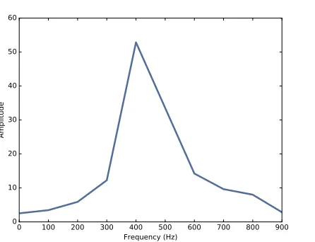
0 2000 4000 6000 8000 10000 Frequency (Hz)

0 500 1000 1500 2000 2500 3000 3500 4000

[image:16.612.167.386.92.266.2]

Amplitude

Figure 1.3: Spectrum of a segment from the violin recording.

The lowest frequency component is called thefundamental frequency. The fundamental frequency of this signal is near 440 Hz (actually a little lower, or “flat”).

In this signal the fundamental frequency has the largest amplitude, so it is also thedominant frequency. Normally the perceived pitch of a sound is determined by the fundamental frequency, even if it is not dominant. The other spikes in the spectrum are at frequencies 880, 1320, 1760, and 2200, which are integer multiples of the fundamental. These components are calledharmonicsbecause they are musically harmonious with the fun-damental:

• 880 is the frequency of A5, one octave higher than the fundamental. Anoctaveis a doubling in frequency.

• 1320 is approximately E6, which is a major fifth above A5. If you are not familiar with musical intervals like "major fifth”, seehttps://en.

wikipedia.org/wiki/Interval_(music). • 1760 is A6, two octaves above the fundamental.

• 2200 is approximately C]7, which is a major third above A6.

(17)

1.3. Signals 5

Given the harmonics and their amplitudes, you can reconstruct the signal by adding up sinusoids. Next we’ll see how.

1.3

Signals

I wrote a Python module calledthinkdsp.pythat contains classes and func-tions for working with signals and spectrums1. You will find it in the repos-itory for this book (see Section 0.2).

To represent signals, thinkdspprovides a class calledSignal, which is the parent class for several signal types, includingSinusoid, which represents both sine and cosine signals.

thinkdspprovides functions to create sine and cosine signals:

cos_sig = thinkdsp.CosSignal(freq=440, amp=1.0, offset=0) sin_sig = thinkdsp.SinSignal(freq=880, amp=0.5, offset=0) freqis frequency in Hz. ampis amplitude in unspecified units where 1.0 is defined as the largest amplitude we can record or play back.

offset is aphase offset in radians. Phase offset determines where in the period the signal starts. For example, a sine signal with offset=0starts at sin 0, which is 0. Withoffset=pi/2it starts at sinπ/2, which is 1.

Signals have an__add__method, so you can use the+operator to add them:

mix = sin_sig + cos_sig

The result is aSumSignal, which represents the sum of two or more signals. A Signal is basically a Python representation of a mathematical function. Most signals are defined for all values oft, from negative infinity to infinity. You can’t do much with a Signal until you evaluate it. In this context, “eval-uate” means taking a sequence of points in time, ts, and computing the corresponding values of the signal,ys. I representtsandysusing NumPy arrays and encapsulate them in an object called a Wave.

A Wave represents a signal evaluated at a sequence of points in time. Each point in time is called a frame(a term borrowed from movies and video). The measurement itself is called asample, although “frame” and “sample” are sometimes used interchangeably.

Signalprovidesmake_wave, which returns a new Wave object:

1_{The plural of “spectrum” is often written “spectra”, but I prefer to use standard English}

(18)

0.000 0.001 0.002 0.003 0.004 0.005 0.006 Time (s)

1.5 1.0 0.5 0.0 0.5 1.0 1.5

Figure 1.4: Segment from a mixture of two sinusoid signals.

wave = mix.make_wave(duration=0.5, start=0, framerate=11025) durationis the length of the Wave in seconds. start is the start time, also in seconds. framerateis the (integer) number of frames per second, which is also the number of samples per second.

11,025 frames per second is one of several framerates commonly used in audio file formats, including Waveform Audio File (WAV) and mp3.

This example evaluates the signal fromt=0tot=0.5at 5,513 equally-spaced frames (because 5,513 is half of 11,025). The time between frames, or timestep, is1/11025seconds, about 91µs.

Waveprovides aplotmethod that uses pyplot. You can plot the wave like this:

wave.plot() pyplot.show()

pyplot is part ofmatplotlib; it is included in many Python distributions, or you might have to install it.

Atfreq=440 there are 220 periods in 0.5 seconds, so this plot would look like a solid block of color. To zoom in on a small number of periods, we can usesegment, which copies a segment of a Wave and returns a new wave:

period = mix.period

segment = wave.segment(start=0, duration=period*3) periodis a property of a Signal; it returns the period in seconds.

(19)

1.4. Reading and writing Waves 7

If we plot segment, it looks like Figure 1.4. This signal contains two fre-quency components, so it is more complicated than the signal from the tun-ing fork, but less complicated than the violin.

1.4

Reading and writing Waves

thinkdspprovidesread_wave, which reads a WAV file and returns a Wave:

violin_wave = thinkdsp.read_wave('input.wav')

AndWaveprovideswrite, which writes a WAV file:

wave.write(filename='output.wav')

You can listen to the Wave with any media player that plays WAV files. On UNIX systems, I use aplay, which is simple, robust, and included in many Linux distributions.

thinkdsp also providesplay_wave, which runs the media player as a sub-process:

thinkdsp.play_wave(filename='output.wav', player='aplay')

It usesaplayby default, but you can provide the name of another player.

1.5

Spectrums

Waveprovidesmake_spectrum, which returns aSpectrum:

spectrum = wave.make_spectrum()

AndSpectrumprovidesplot:

spectrum.plot() thinkplot.show()

thinkplot is a module I wrote to provide wrappers around some of the functions in pyplot. It is included in the Git repository for this book (see Section 0.2).

Spectrumprovides three methods that modify the spectrum:

(20)

Wave Spectrum Signal

Figure 1.5: Relationships among the classes inthinkdsp.

• high_pass applies a high-pass filter, which means that it attenuates components below the cutoff.

• band_stopattenuates components in the band of frequencies between two cutoffs.

This example attenuates all frequencies above 600 by 99%:

spectrum.low_pass(cutoff=600, factor=0.01)

A low pass filter removes bright, high-frequency sounds, so the result sounds muffled and darker. To hear what it sounds like, you can convert the Spectrum back to a Wave, and then play it.

wave = spectrum.make_wave() wave.play('temp.wav')

The play method writes the wave to a file and then plays it. If you use Jupyter notebooks, you can usemake_audio, which makes an Audio widget that plays the sound.

1.6

Wave objects

There is nothing very complicated inthinkdsp.py. Most of the functions it provides are thin wrappers around functions from NumPy and SciPy. The primary classes inthinkdspare Signal, Wave, and Spectrum. Given a Signal, you can make a Wave. Given a Wave, you can make a Spectrum, and vice versa. These relationships are shown in Figure 1.5.

A Wave object contains three attributes: ysis a NumPy array that contains the values in the signal; ts is an array of the times where the signal was evaluated or sampled; andframerateis the number of samples per unit of time. The unit of time is usually seconds, but it doesn’t have to be. In one of my examples, it’s days.

Wave also provides three read-only properties:start,end, andduration. If you modifyts, these properties change accordingly.

(21)

1.7. Signal objects 9

wave.ys *= 2 wave.ts += 1

The first line scales the wave by a factor of 2, making it louder. The second line shifts the wave in time, making it start 1 second later.

But Wave provides methods that perform many common operations. For example, the same two transformations could be written:

wave.scale(2) wave.shift(1)

You can read the documentation of these methods and others at http://

greenteapress.com/thinkdsp.html.

1.7

Signal objects

Signal is a parent class that provides functions common to all kinds of signals, like make_wave. Child classes inherit these methods and provide

evaluate, which evaluates the signal at a given sequence of times. For example, Sinusoid is a child class of Signal, with this definition:

class Sinusoid(Signal):

def __init__(self, freq=440, amp=1.0, offset=0, func=np.sin): Signal.__init__(self)

self.freq = freq self.amp = amp

self.offset = offset self.func = func

The parameters of__init__are:

• freq: frequency in cycles per second, or Hz.

• amp: amplitude. The units of amplitude are arbitrary, usually chosen so 1.0 corresponds to the maximum input from a microphone or max-imum output to a speaker.

• offset: indicates where in its period the signal starts; offset is in units of radians, for reasons I explain below.

(22)

Like many init methods, this one just tucks the parameters away for future use.

Signal providesmake_wave, which looks like this:

def make_wave(self, duration=1, start=0, framerate=11025): n = round(duration * framerate)

ts = start + np.arange(n) / framerate ys = self.evaluate(ts)

return Wave(ys, ts, framerate=framerate)

startanddurationare the start time and duration in seconds. framerate is the number of frames (samples) per second.

nis the number of samples, andtsis a NumPy array of sample times. To compute theys,make_waveinvokesevaluate, is provided bySinusoid:

def evaluate(self, ts):

phases = PI2 * self.freq * ts + self.offset ys = self.amp * self.func(phases)

return ys

Let’s unwind this function one step at time:

1. self.freq is frequency in cycles per second, and each element of ts is a time in seconds, so their product is the number of cycles since the start time.

2. PI2 is a constant that stores 2π. Multiplying by PI2 converts from

cycles tophase. You can think of phase as “cycles since the start time” expressed in radians. Each cycle is 2πradians.

3. self.offset is the phase when t = 0. It has the effect of shifting the signal left or right in time.

4. Ifself.funcisnp.sinornp.cos, the result is a value between−1 and

+1.

5. Multiplying by self.ampyields a signal that ranges from -self.amp to+self.amp.

In math notation,evaluateis written like this:

y = Acos(2πf t+φ0)

(23)

1.8. Exercises 11

1.8

Exercises

Before you begin these exercises, you should download the code for this book, following the instructions in Section 0.2.

Solutions to these exercises are inchap01soln.ipynb.

Exercise 1.1If you have Jupyter, load chap01.ipynb, read through it, and run the examples. You can also view this notebook at http://tinyurl.

com/thinkdsp01.

Exercise 1.2Go to http://freesound.org and download a sound sample that includes music, speech, or other sounds that have a well-defined pitch. Select a roughly half-second segment where the pitch is constant. Compute and plot the spectrum of the segment you selected. What connection can you make between the timbre of the sound and the harmonic structure you see in the spectrum?

Usehigh_pass, low_pass, andband_stopto filter out some of the harmon-ics. Then convert the spectrum back to a wave and listen to it. How does the sound relate to the changes you made in the spectrum?

Exercise 1.3Synthesize a compound signal by creating SinSignal and CosSignal objects and adding them up. Evaluate the signal to get a Wave, and listen to it. Compute its Spectrum and plot it. What happens if you add frequency components that are not multiples of the fundamental?

Exercise 1.4Write a function calledstretchthat takes a Wave and a stretch factor and speeds up or slows down the wave by modifying ts and

(24)

(25)

Chapter 2

Harmonics

In this chapter I present several new waveforms; we will look and their spectrums to understand theirharmonic structure, which is the set of sinu-soids they are made up of.

I’ll also introduce one of the most important phenomena in digital signal processing: aliasing. And I’ll explain a little more about how the Spectrum class works.

thinkdsp02.

2.1

Triangle waves

A sinusoid contains only one frequency component, so its spectrum has only one peak. More complicated waveforms, like the violin recording, yield DFTs with many peaks. In this section we investigate the relationship between waveforms and their spectrums.

I’ll start with a triangle waveform, which is like a straight-line version of a sinusoid. Figure 2.1 shows a triangle waveform with frequency 200 Hz. To generate a triangle wave, you can usethinkdsp.TriangleSignal:

class TriangleSignal(Sinusoid):

(26)

0.000 0.002 0.004 0.006 0.008 0.010 0.012 0.014 Time (s)

1.0 0.5 0.0 0.5 1.0

Figure 2.1: Segment of a triangle signal at 200 Hz.

frac, _ = np.modf(cycles) ys = np.abs(frac - 0.5)

ys = normalize(unbias(ys), self.amp) return ys

TriangleSignalinherits __init__from Sinusoid, so it takes the same ar-guments:freq,amp, andoffset.

The only difference is evaluate. As we saw before, ts is the sequence of sample times where we want to evaluate the signal.

There are many ways to generate a triangle wave. The details are not im-portant, but here’s howevaluateworks:

1. cycles is the number of cycles since the start time. np.modfsplits the number of cycles into the fraction part, stored infrac, and the integer part, which is ignored1.

2. frac is a sequence that ramps from 0 to 1 with the given frequency. Subtracting 0.5 yields values between -0.5 and 0.5. Taking the absolute value yields a waveform that zig-zags between 0.5 and 0.

3. unbiasshifts the waveform down so it is centered at 0; thennormalize scales it to the given amplitude,amp.

Here’s the code that generates Figure 2.1:

(27)

2.1. Triangle waves 15

0 1000 2000 3000 4000 5000 Frequency (Hz)

0 500 1000 1500 2000 2500

Amplitude

0 1000 2000 3000 4000 5000 Frequency (Hz)

0 100 200 300 400 500

Figure 2.2: Spectrum of a triangle signal at 200 Hz, shown on two verti-cal sverti-cales. The version on the right cuts off the fundamental to show the harmonics more clearly.

Next we can use the Signal to make a Wave, and use the Wave to make a Spectrum:

wave = signal.make_wave(duration=0.5, framerate=10000) spectrum = wave.make_spectrum()

spectrum.plot()

Figure 2.2 shows two views of the result; the view on the right is scaled to show the harmonics more clearly. As expected, the highest peak is at the fundamental frequency, 200 Hz, and there are additional peaks at harmonic frequencies, which are integer multiples of 200.

But one surprise is that there are no peaks at the even multiples: 400, 800, etc. The harmonics of a triangle wave are all odd multiples of the funda-mental frequency, in this example 600, 1000, 1400, etc.

Another feature of this spectrum is the relationship between the amplitude and frequency of the harmonics. Their amplitude drops off in proportion to frequency squared. For example the frequency ratio of the first two har-monics (200 and 600 Hz) is 3, and the amplitude ratio is approximately 9. The frequency ratio of the next two harmonics (600 and 1000 Hz) is 1.7, and the amplitude ratio is approximately 1.72 = 2.9. This relationship is called theharmonic structure.

1_{Using an underscore as a variable name is a convention that means, “I don’t intend to}

(28)

0.000 0.005 0.010 0.015 0.020 0.025 0.030 Time (s)

1.0 0.5 0.0 0.5 1.0

Figure 2.3: Segment of a square signal at 100 Hz.

2.2

Square waves

thinkdsp also provides SquareSignal, which represents a square signal. Here’s the class definition:

class SquareSignal(Sinusoid):

cycles = self.freq * ts + self.offset / PI2 frac, _ = np.modf(cycles)

ys = self.amp * np.sign(unbias(frac)) return ys

LikeTriangleSignal,SquareSignalinherits__init__fromSinusoid, so it takes the same parameters.

And theevaluatemethod is similar. Again,cyclesis the number of cycles since the start time, andfracis the fractional part, which ramps from 0 to 1 each period.

unbiasshiftsfracso it ramps from -0.5 to 0.5, thennp.signmaps the neg-ative values to -1 and the positive values to 1. Multiplying byampyields a square wave that jumps between-ampandamp.

Figure 2.3 shows three periods of a square wave with frequency 100 Hz, and Figure 2.4 shows its spectrum.

(29)

2.3. Aliasing 17

0 1000 2000 3000 4000 5000

Frequency (Hz) 0

500 1000 1500 2000 2500 3000 3500

Amplitude

Figure 2.4: Spectrum of a square signal at 100 Hz.

harmonics drops off more slowly. Specifically, amplitude drops in propor-tion to frequency (not frequency squared).

The exercises at the end of this chapter give you a chance to explore other waveforms and other harmonic structures.

2.3

Aliasing

I have a confession. I chose the examples in the previous section carefully to avoid showing you something confusing. But now it’s time to get confused. Figure 2.5 shows the spectrum of a triangle wave at 1100 Hz, sampled at 10,000 frames per second. Again, the view on the right is scaled to show the harmonics.

The harmonics of this wave should be at 3300, 5500, 7700, and 9900 Hz. In the figure, there are peaks at 1100 and 3300 Hz, as expected, but the third peak is at 4500, not 5500 Hz. The fourth peak is at 2300, not 7700 Hz. And if you look closely, the peak that should be at 9900 is actually at 100 Hz. What’s going on?

(30)

0 1000 2000 3000 4000 5000 Frequency (Hz)

0 500 1000 1500 2000 2500

Amplitude

0 1000 2000 3000 4000 5000 Frequency (Hz)

0 100 200 300 400 500

Figure 2.5: Spectrum of a triangle signal at 1100 Hz sampled at 10,000 frames per second. The view on the right is scaled to show the harmon-ics.

But if you sample a signal at 5000 Hz with 10,000 frames per second, you only have two samples per period. That turns out to be enough, just barely, but if the frequency is higher, it’s not.

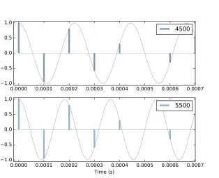
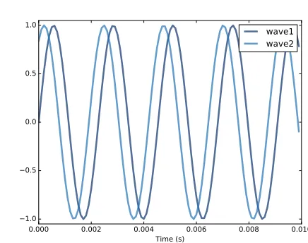
To see why, let’s generate cosine signals at 4500 and 5500 Hz, and sample them at 10,000 frames per second:

framerate = 10000

signal = thinkdsp.CosSignal(4500) duration = signal.period*5

segment = signal.make_wave(duration, framerate=framerate) segment.plot()

signal = thinkdsp.CosSignal(5500)

segment = signal.make_wave(duration, framerate=framerate) segment.plot()

Figure 2.6 shows the result. I plotted the Signals with thin gray lines and the samples using vertical lines, to make it easier to compare the two Waves. The problem should be clear: even though the Signals are different, the Waves are identical!

(31)

2.4. Computing the spectrum 19

0.0000 0.0001 0.0002 0.0003 0.0004 0.0005 0.0006 0.0007 1.0

0.5 0.0 0.5 1.0

4500

0.0000 0.0001 0.0002 0.0003 0.0004 0.0005 0.0006 0.0007 Time (s)

1.0 0.5 0.0 0.5 1.0

[image:31.612.182.496.84.340.2]

5500

Figure 2.6: Cosine signals at 4500 and 5500 Hz, sampled at 10,000 frames per second. The signals are different, but the samples are identical.

This effect is calledaliasingbecause when the high frequency signal is sam-pled, it appears to be a low frequency signal.

In this example, the highest frequency we can measure is 5000 Hz, which is half the sampling rate. Frequencies above 5000 Hz are folded back be-low 5000 Hz, which is why this threshold is sometimes called the “fold-ing frequency”. It is sometimes also called the Nyquist frequency. See

http://en.wikipedia.org/wiki/Nyquist_frequency.

The folding pattern continues if the aliased frequency goes below zero. For example, the 5th harmonic of the 1100 Hz triangle wave is at 12,100 Hz. Folded at 5000 Hz, it would appear at -2100 Hz, but it gets folded again at 0 Hz, back to 2100 Hz. In fact, you can see a small peak at 2100 Hz in Figure 2.4, and the next one at 4300 Hz.

2.4

Computing the spectrum

(32)

from np.fft import rfft, rfftfreq

# class Wave:

def make_spectrum(self): n = len(self.ys)

d = 1 / self.framerate

hs = rfft(self.ys) fs = rfftfreq(n, d)

return Spectrum(hs, fs, self.framerate)

The parameter self is a Wave object. n is the number of samples in the wave, and d is the inverse of the frame rate, which is the time between samples.

np.fft is the NumPy module that provides functions related to the Fast Fourier Transform(FFT), which is an efficient algorithm that computes the Discrete Fourier Transform (DFT).

make_spectrum usesrfft, which stands for “real FFT”, because the Wave contains real values, not complex. Later we’ll see the full FFT, which can handle complex signals. The result of rfft, which I call hs, is a NumPy array of complex numbers that represents the amplitude and phase offset of each frequency component in the wave.

The result ofrfftfreq, which I callfs, is an array that contains frequencies corresponding to thehs.

To understand the values in hs, consider these two ways to think about complex numbers:

• A complex number is the sum of a real part and an imaginary part, often written x+iy, where i is the imaginary unit, √−1. You can think of xandyas Cartesian coordinates.

• A complex number is also the product of a magnitude and a complex exponential, Aeiφ_{, where} _A _{is the} _magnitude _and

φ is the angle in

radians, also called the “argument”. You can think of Aandφas polar

coordinates.

(33)

2.5. Exercises 21

The Spectrum class provides two read-only properties, amps and angles, which return NumPy arrays representing the magnitudes and angles of the

hs. When we plot a Spectrum object, we usually plotampsversusfs. Some-times it is also useful to plotanglesversusfs.

Although it might be tempting to look at the real and imaginary parts of

hs, you will almost never need to. I encourage you to think of the DFT as a vector of amplitudes and phase offsets that happen to be encoded in the form of complex numbers.

To modify a Spectrum, you can access thehsdirectly. For example:

spectrum.hs *= 2

spectrum.hs[spectrum.fs > cutoff] = 0

The first line multiples the elements of hs by 2, which doubles the ampli-tudes of all components. The second line sets to 0 only the elements of hs where the corresponding frequency exceeds some cutoff frequency.

But Spectrum also provides methods to perform these operations:

spectrum.scale(2)

spectrum.low_pass(cutoff)

You can read the documentation of these methods and others at http://

greenteapress.com/thinkdsp.html.

At this point you should have a better idea of how the Signal, Wave, and Spectrum classes work, but I have not explained how the Fast Fourier Trans-form works. That will take a few more chapters.

2.5

Exercises

Exercise 2.1If you use Jupyter, loadchap02.ipynband try out the examples. You can also view the notebook athttp://tinyurl.com/thinkdsp02. Exercise 2.2A sawtooth signal has a waveform that ramps up linearly from -1 to 1, then drops to -1 and repeats. See http://en.wikipedia.org/wiki/

Sawtooth_wave

Write a class called SawtoothSignal that extends Signal and provides

evaluateto evaluate a sawtooth signal.

(34)

Exercise 2.3Make a square signal at 1100 Hz and make a wave that samples it at 10000 frames per second. If you plot the spectrum, you can see that most of the harmonics are aliased. When you listen to the wave, can you hear the aliased harmonics?

Exercise 2.4If you have a spectrum object,spectrum, and print the first few values ofspectrum.fs, you’ll see that they start at zero. Sospectrum.hs[0] is the magnitude of the component with frequency 0. But what does that mean?

Try this experiment:

1. Make a triangle signal with frequency 440 and make a Wave with du-ration 0.01 seconds. Plot the waveform.

2. Make a Spectrum object and print spectrum.hs[0]. What is the am-plitude and phase of this component?

3. Set spectrum.hs[0] = 100. Make a Wave from the modified Spec-trum and plot it. What effect does this operation have on the wave-form?

Exercise 2.5Write a function that takes a Spectrum as a parameter and modifies it by dividing each element ofhs by the corresponding frequency from fs. Hint: since division by zero is undefined, you might want to set

spectrum.hs[0] = 0.

Test your function using a square, triangle, or sawtooth wave. 1. Compute the Spectrum and plot it.

2. Modify the Spectrum using your function and plot it again.

3. Make a Wave from the modified Spectrum and listen to it. What effect does this operation have on the signal?

Exercise 2.6Triangle and square waves have odd harmonics only; the saw-tooth wave has both even and odd harmonics. The harmonics of the square and sawtooth waves drop off in proportion to 1/f; the harmonics of the tri-angle wave drop off like 1/f2. Can you find a waveform that has even and odd harmonics that drop off like 1/f2?

(35)

Chapter 3

Non-periodic signals

The signals we have worked with so far are periodic, which means that they repeat forever. It also means that the frequency components they contain do not change over time. In this chapter, we consider non-periodic signals, whose frequency components dochange over time. In other words, pretty much all sound signals.

This chapter also presents spectrograms, a common way to visualize non-periodic signals.

thinkdsp03.

3.1

Linear chirp

We’ll start with achirp, which is a signal with variable frequency. thinkdsp provides a Signal called Chirp that makes a sinusoid that sweeps linearly through a range of frequencies.

Here’s an example that sweeps from 220 to 880 Hz, which is two octaves from A3 to A5:

signal = thinkdsp.Chirp(start=220, end=880) wave = signal.make_wave()

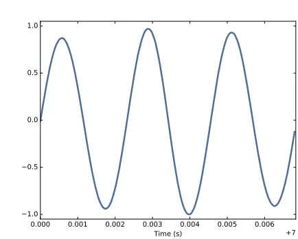
Figure 3.1 shows segments of this wave near the beginning, middle, and end. It’s clear that the frequency is increasing.

(36)

0 2 4 6 8 10 1.0

0.5 0.0 0.5 1.0

500 502 504 506 508 510

Time (ms) 900 902 904 906 908 910

Figure 3.1: Chirp waveform near the beginning, middle, and end.

class Chirp(Signal):

def __init__(self, start=440, end=880, amp=1.0): self.start = start

self.end = end self.amp = amp

startand endare the frequencies, in Hz, at the start and end of the chirp.

ampis amplitude.

Here is the function that evaluates the signal:

freqs = np.linspace(self.start, self.end, len(ts)-1) return self._evaluate(ts, freqs)

ts is the sequence of points in time where the signal should be evaluated; to keep this function simple, I assume they are equally-spaced.

If the length oftsis n, you can think of it as a sequence of n−1 intervals of time. To compute the frequency during each interval, I usenp.linspace, which returns a NumPy array ofn−1 values betweenstartandend.

_evaluateis a private method that does the rest of the math1:

def _evaluate(self, ts, freqs): dts = np.diff(ts)

dphis = PI2 * freqs * dts

1_{Beginning a method name with an underscore makes it “private”, indicating that it is}

(37)

3.1. Linear chirp 25

phases = np.cumsum(dphis)

phases = np.insert(phases, 0, 0) ys = self.amp * np.cos(phases) return ys

np.diffcomputes the difference between adjacent elements ofts, returning the length of each interval in seconds. If the elements of ts are equally spaced, thedtsare all the same.

The next step is to figure out how much the phase changes during each interval. In Section 1.7 we saw that when frequency is constant, the phase,

φ, increases linearly over time:

φ=2πf t

When frequency is a function of time, the change in phase during a short time interval,∆tis:

∆φ=2πf(t)∆t

In Python, sincefreqscontains f(t)anddtscontains the time intervals, we can write

dphis = PI2 * freqs * dts

Now, sincedphiscontains the changes in phase, we can get the total phase at each timestep by adding up the changes:

phases = np.cumsum(dphis)

phases = np.insert(phases, 0, 0)

np.cumsum computes the cumulative sum, which is almost what we want, but it doesn’t start at 0. So I usenp.insertto add a 0 at the beginning. The result is a NumPy array where theith element contains the sum of the firstiterms fromdphis; that is, the total phase at the end of theith interval. Finally, np.coscomputes the amplitude of the wave as a function of phase (remember that phase is expressed in radians).

If you know calculus, you might notice that the limit as∆tgets small is

dφ=2πf(t)dt

Dividing through bydtyields

dφ

dt =2πf(t)

(38)

the integral of frequency. When we used cumsum to go from frequency to phase, we were approximating integration.

3.2

Exponential chirp

When you listen to this chirp, you might notice that the pitch rises quickly at first and then slows down. The chirp spans two octaves, but it only takes 2/3 s to span the first octave, and twice as long to span the second.

The reason is that our perception of pitch depends on the logarithm of fre-quency. As a result, theintervalwe hear between two notes depends on the

ratioof their frequencies, not the difference. “Interval” is the musical term for the perceived difference between two pitches.

For example, an octave is an interval where the ratio of two pitches is 2. So the interval from 220 to 440 is one octave and the interval from 440 to 880 is also one octave. The difference in frequency is bigger, but the ratio is the same.

As a result, if frequency increases linearly, as in a linear chirp, the perceived pitch increases logarithmically.

If you want the perceived pitch to increase linearly, the frequency has to increase exponentially. A signal with that shape is called an exponential chirp.

Here’s the code that makes one:

class ExpoChirp(Chirp):

start, end = np.log10(self.start), np.log10(self.end) freqs = np.logspace(start, end, len(ts)-1)

return self._evaluate(ts, freqs)

Instead of np.linspace, this version of evaluate usesnp.logspace, which creates a series of frequencies whose logarithms are equally spaced, which means that they increase exponentially.

That’s it; everything else is the same as Chirp. Here’s the code that makes one:

signal = thinkdsp.ExpoChirp(start=220, end=880) wave = signal.make_wave(duration=1)

(39)

3.3. Spectrum of a chirp 27

0 100 200 300 400 500 600 700 Frequency (Hz)

0 50 100 150 200 250 300 350 400 450

Amplitude

Figure 3.2: Spectrum of a one-second one-octave chirp.

3.3

Spectrum of a chirp

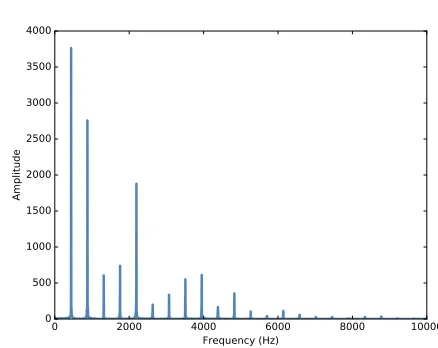
What do you think happens if you compute the spectrum of a chirp? Here’s an example that constructs a one-second, one-octave chirp and its spectrum:

signal = thinkdsp.Chirp(start=220, end=440) wave = signal.make_wave(duration=1)

Figure 3.2 shows the result. The spectrum has components at every fre-quency from 220 to 440 Hz, with variations that look a little like the Eye of Sauron (seehttp://en.wikipedia.org/wiki/Sauron).

The spectrum is approximately flat between 220 and 440 Hz, which in-dicates that the signal spends equal time at each frequency in this range. Based on that observation, you should be able to guess what the spectrum of an exponential chirp looks like.

The spectrum gives hints about the structure of the signal, but it obscures the relationship between frequency and time. For example, we cannot tell by looking at this spectrum whether the frequency went up or down, or both.

3.4

Spectrogram

(40)

0.0 0.2 0.4 0.6 0.8 1.0 Time (s)

0 100 200 300 400 500 600 700

Frequency (Hz)

Figure 3.3: Spectrogram of a one-second one-octave chirp.

There are several ways to visualize a STFT, but the most common is a spec-trogram, which shows time on the x-axis and frequency on the y-axis. Each column in the spectrogram shows the spectrum of a short segment, using color or grayscale to represent amplitude.

As an example, I’ll compute the spectrogram of this chirp:

signal = thinkdsp.Chirp(start=220, end=440)

wave = signal.make_wave(duration=1, framerate=11025)

Waveprovidesmake_spectrogram, which returns aSpectrogramobject:

spectrogram = wave.make_spectrogram(seg_length=512) spectrogram.plot(high=700)

seg_lengthis the number of samples in each segment. I chose 512 because FFT is most efficient when the number of samples is a power of 2.

Figure 3.3 shows the result. The x-axis shows time from 0 to 1 seconds. The y-axis shows frequency from 0 to 700 Hz. I cut off the top part of the spectrogram; the full range goes to 5512.5 Hz, which is half of the framerate. The spectrogram shows clearly that frequency increases linearly over time. Similarly, in the spectrogram of an exponential chirp, we can see the shape of the exponential curve.

(41)

3.5. The Gabor limit 29

3.5

The Gabor limit

The time resolution of the spectrogram is the duration of the segments, which corresponds to the width of the cells in the spectrogram. Since each segment is 512 frames, and there are 11,025 frames per second, the duration of each segment is about 0.046 seconds.

The frequency resolution is the frequency range between elements in the spectrum, which corresponds to the height of the cells. With 512 frames, we get 256 frequency components over a range from 0 to 5512.5 Hz, so the range between components is 21.6 Hz.

More generally, ifnis the segment length, the spectrum contains n/2 com-ponents. If the framerate is r, the maximum frequency in the spectrum is

r/2. So the time resolution isn/rand the frequency resolution is

r/2

n/2 which isr/n.

Ideally we would like time resolution to be small, so we can see rapid changes in frequency. And we would like frequency resolution to be small so we can see small changes in frequency. But you can’t have both. Notice that time resolution, n/r, is the inverse of frequency resolution,r/n. So if one gets smaller, the other gets bigger.

For example, if you double the segment length, you cut frequency resolu-tion in half (which is good), but you double time resoluresolu-tion (which is bad). Even increasing the framerate doesn’t help. You get more samples, but the range of frequencies increases at the same time.

This tradeoff is called theGabor limitand it is a fundamental limitation of this kind of time-frequency analysis.

3.6

Leakage

In order to explain how make_spectrogram works, I have to explain win-dowing; and in order to explain windowing, I have to show you the prob-lem it is meant to address, which is leakage.

(42)

0 200 400 600 800 0 50 100 150 200 250 300 350 400

0 200 400 600 800 Frequency (Hz) 0 50 100 150 200 250 300 350

0 200 400 600 800 0

[image:42.612.88.469.63.301.2]

50 100 150 200

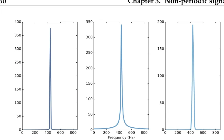
Figure 3.4: Spectrum of a periodic segment of a sinusoid (left), a non-periodic segment (middle), a windowed non-non-periodic segment (right).

it operates on is a complete period from an infinite signal that repeats over all time. In practice, this assumption is often false, which creates problems. One common problem is discontinuity at the beginning and end of the seg-ment. Because DFT assumes that the signal is periodic, it implicitly connects the end of the segment back to the beginning to make a loop. If the end does not connect smoothly to the beginning, the discontinuity creates additional frequency components in the segment that are not in the signal.

As an example, let’s start with a sine signal that contains only one frequency component at 440 Hz.

signal = thinkdsp.SinSignal(freq=440)

If we select a segment that happens to be an integer multiple of the period, the end of the segment connects smoothly with the beginning, and DFT behaves well.

duration = signal.period * 30 wave = signal.make_wave(duration) spectrum = wave.make_spectrum()

Figure 3.4 (left) shows the result. As expected, there is a single peak at 440 Hz.

But if the duration is not a multiple of the period, bad things happen. With

(43)

3.7. Windowing 31

0.000 0.005 0.010 0.015 0.020 1.0

0.5 0.0 0.5 1.0

0.000 0.005 0.010 0.015 0.020 1.0

0.5 0.0 0.5 1.0

0.000 0.005 0.010 0.015 0.020 Time (s)

[image:43.612.236.420.97.340.2]

1.0 0.5 0.0 0.5 1.0

Figure 3.5: Segment of a sinusoid (top), Hamming window (middle), prod-uct of the segment and the window (bottom).

Figure 3.4 (middle) shows the spectrum of this segment. Again, the peak is at 440 Hz, but now there are additional components spread out from 240 to 640 Hz. This spread is called spectral leakage, because some of the energy that is actually at the fundamental frequency leaks into other frequencies. In this example, leakage happens because we are using DFT on a segment that becomes discontinuous when we treat it as periodic.

3.7

Windowing

We can reduce leakage by smoothing out the discontinuity between the be-ginning and end of the segment, and one way to do that iswindowing. A “window” is a function designed to transform a non-periodic segment into something that can pass for periodic. Figure 3.5 (top) shows a segment where the end does not connect smoothly to the beginning.

(44)

0 100 200 300 400 500 600 700 800 Index

0.0 0.2 0.4 0.6 0.8 1.0

Figure 3.6: Overlapping Hamming windows.

Figure 3.5 (bottom) shows the result of multiplying the window by the orig-inal signal. Where the window is close to 1, the signal is unchanged. Where the window is close to 0, the signal is attenuated. Because the window tapers at both ends, the end of the segment connects smoothly to the begin-ning.

Figure 3.4 (right) shows the spectrum of the windowed signal. Windowing has reduced leakage substantially, but not completely.

Here’s what the code looks like. Wave provides window, which applies a Hamming window:

#class Wave:

def window(self, window): self.ys *= window

And NumPy provideshamming, which computes a Hamming window with a given length:

window = np.hamming(len(wave)) wave.window(window)

NumPy provides functions to compute other window functions, including

bartlett, blackman, hanning, andkaiser. One of the exercises at the end of this chapter asks you to experiment with these other windows.

3.8

Implementing spectrograms

(45)

3.8. Implementing spectrograms 33

#class Wave:

def make_spectrogram(self, seg_length): window = np.hamming(seg_length) i, j = 0, seg_length

step = seg_length / 2

spec_map = {}

while j < len(self.ys):

segment = self.slice(i, j) segment.window(window)

t = (segment.start + segment.end) / 2 spec_map[t] = segment.make_spectrum()

i += step j += step

return Spectrogram(spec_map, seg_length)

This is the longest function in the book, so if you can handle this, you can handle anything.

The parameter,self, is a Wave object.seg_lengthis the number of samples in each segment.

windowis a Hamming window with the same length as the segments.

i and j are the slice indices that select segments from the wave. step is the offset between segments. Sincestepis half ofseg_length, the segments overlap by half. Figure 3.6 shows what these overlapping windows look like.

spec_mapis a dictionary that maps from a timestamp to a Spectrum.

Inside the while loop, we select a slice from the wave and apply the win-dow; then we construct a Spectrum object and add it tospec_map. The nom-inal time of each segment,t, is the midpoint.

Then we advanceiandj, and continue as long asjdoesn’t go past the end of the Wave.

(46)

class Spectrogram(object):

def __init__(self, spec_map, seg_length): self.spec_map = spec_map

self.seg_length = seg_length

Like many init methods, this one just stores the parameters as attributes.

Spectrogramprovidesplot, which generates a pseudocolor plot with time along the x-axis and frequency along the y-axis.

And that’s how Spectrograms are implemented.

3.9

Exercises

Exercise 3.1Run and listen to the examples inchap03.ipynb, which is in the repository for this book, and also available at http://tinyurl.com/

thinkdsp03.

In the leakage example, try replacing the Hamming window with one of the other windows provided by NumPy, and see what effect they have on leakage. See http://docs.scipy.org/doc/numpy/reference/routines.

window.html

Exercise 3.2Write a class called SawtoothChirp that extends Chirp and overridesevaluate to generate a sawtooth waveform with frequency that increases (or decreases) linearly.

Hint: combine the evaluate functions fromChirpandSawtoothSignal. Draw a sketch of what you think the spectrogram of this signal looks like, and then plot it. The effect of aliasing should be visually apparent, and if you listen carefully, you can hear it.

Exercise 3.3Make a sawtooth chirp that sweeps from 2500 to 3000 Hz, then use it to make a wave with duration 1 s and framerate 20 kHz. Draw a sketch of what you think the spectrum will look like. Then plot the spec-trum and see if you got it right.

Exercise 3.4In musical terminology, a “glissando” is a note that slides from one pitch to another, so it is similar to a chirp.

Find or make a recording of a glissando and plot a spectrogram of the first few seconds. One suggestion: George Gershwin’s Rhapsody in Blue starts with a famous clarinet glissando, which you can download fromhttp://

(47)

3.9. Exercises 35

Exercise 3.5A trombone player can play a glissando by extending the trom-bone slide while blowing continuously. As the slide extends, the total length of the tube gets longer, and the resulting pitch is inversely proportional to length.

Assuming that the player moves the slide at a constant speed, how does frequency vary with time?

Write a class called TromboneGliss that extends Chirp and provides

evaluate. Make a wave that simulates a trombone glissando from C3 up to F3 and back down to C3. C3 is 262 Hz; F3 is 349 Hz.

Plot a spectrogram of the resulting wave. Is a trombone glissando more like a linear or exponential chirp?

(48)

(49)

Chapter 4

Noise

In English, “noise” means an unwanted or unpleasant sound. In the context of signal processing, it has two different senses:

1. As in English, it can mean an unwanted signal of any kind. If two signals interfere with each other, each signal would consider the other to be noise.

2. “Noise” also refers to a signal that contains components at many fre-quencies, so it lacks the harmonic structure of the periodic signals we saw in previous chapters.

This chapter is about the second kind.

thinkdsp04.

4.1

Uncorrelated noise

The simplest way to understand noise is to generate it, and the simplest kind to generate is uncorrelated uniform noise (UU noise). “Uniform” means the signal contains random values from a uniform distribution; that is, every value in the range is equally likely. “Uncorrelated” means that the values are independent; that is, knowing one value provides no information about the others.

(50)

0.00 0.02 0.04 0.06 0.08 0.10 Time (s)

1.0 0.5 0.0 0.5 1.0

Figure 4.1: Waveform of uncorrelated uniform noise.

class UncorrelatedUniformNoise(_Noise):

ys = np.random.uniform(-self.amp, self.amp, len(ts)) return ys

UncorrelatedUniformNoise inherits from _Noise, which inherits from

Signal.

As usual, the evaluate function takests, the times when the signal should be evaluated. It uses np.random.uniform, which generates values from a uniform distribution. In this example, the values are in the range between

-amptoamp.

The following example generates UU noise with duration 0.5 seconds at 11,025 samples per second.

signal = thinkdsp.UncorrelatedUniformNoise()

wave = signal.make_wave(duration=0.5, framerate=11025)

If you play this wave, it sounds like the static you hear if you tune a ra-dio between channels. Figure 4.1 shows what the waveform looks like. As expected, it looks pretty random.

Now let’s take a look at the spectrum:

spectrum = wave.make_spectrum() spectrum.plot_power()

(51)

switch-4.1. Uncorrelated noise 39

0 1000 2000 3000 4000 5000 Frequency (Hz)

0 2000 4000 6000 8000 10000 12000 14000 16000

Power

Figure 4.2: Power spectrum of uncorrelated uniform noise.

ing from amplitude to power in this chapter because it is more conventional in the context of noise.

Figure 4.2 shows the result. Like the signal, the spectrum looks pretty ran-dom. In fact, it israndom, but we have to be more precise about the word “random”. There are at least three things we might like to know about a noise signal or its spectrum:

• Distribution: The distribution of a random signal is the set of possible values and their probabilities. For example, in the uniform noise sig-nal, the set of values is the range from -1 to 1, and all values have the same probability. An alternative is Gaussian noise, where the set of values is the range from negative to positive infinity, but values near 0 are the most likely, with probability that drops off according to the Gaussian or “bell” curve.

• Correlation: Is each value in the signal independent of the others, or are there dependencies between them? In UU noise, the values are independent. An alternative isBrownian noise, where each value is the sum of the previous value and a random “step”. So if the value of the signal is high at a particular point in time, we expect it to stay high, and if it is low, we expect it to stay low.

(52)

0 1000 2000 3000 4000 5000 Frequency (Hz)

0.0 0.2 0.4 0.6 0.8 1.0

Cumulative fraction of total power

Figure 4.3: Integrated spectrum of uncorrelated uniform noise.

that is, the power at frequency f is drawn from a distribution whose mean is proportional to 1/f.

4.2

Integrated spectrum

For UU noise we can see the relationship between power and frequency more clearly by looking at theintegrated spectrum, which is a function of frequency, f, that shows the cumulative power in the spectrum up to f.

Spectrumprovides a method that computes the IntegratedSpectrum:

def make_integrated_spectrum(self): cs = np.cumsum(self.power) cs /= cs[-1]

return IntegratedSpectrum(cs, self.fs)

self.power is a NumPy array containing power for each frequency.

np.cumsumcomputes the cumulative sum of the powers. Dividing through by the last element normalizes the integrated spectrum so it runs from 0 to 1.

The result is an IntegratedSpectrum. Here is the class definition:

class IntegratedSpectrum(object): def __init__(self, cs, fs):

(53)

4.3. Brownian noise 41

0.00 0.02 0.04 0.06 0.08 0.10

Time (s) 1.0

0.5 0.0 0.5 1.0

Figure 4.4: Waveform of Brownian noise.

Like Spectrum, IntegratedSpectrum provides plot_power, so we can com-pute and plot the integrated spectrum like this:

integ = spectrum.make_integrated_spectrum() integ.plot_power()

The result, shown in Figure 4.3, is a straight line, which indicates that power at all frequencies is constant, on average. Noise with equal power at all frequencies is called white noise by analogy with light, because an equal mixture of light at all visible frequencies is white.

4.3

Brownian noise

UU noise is uncorrelated, which means that each value does not depend on the others. An alternative is Brownian noise, in which each value is the sum of the previous value and a random “step”.

It is called “Brownian” by analogy with Brownian motion, in which a parti-cle suspended in a fluid moves apparently at random, due to unseen inter-actions with the fluid. Brownian motion is often described using arandom walk, which is a mathematical model of a path where the distance between steps is characterized by a random distribution.

(54)

This observation suggests a way to generate Brownian noise: generate un-correlated random steps and then add them up. Here is a class definition that implements this algorithm:

class BrownianNoise(_Noise):

dys = np.random.uniform(-1, 1, len(ts)) ys = np.cumsum(dys)

ys = normalize(unbias(ys), self.amp) return ys

evaluateuses np.random.uniformto generate an uncorrelated signal and

np.cumsumto compute their cumulative sum.

Since the sum is likely to escape the range from -1 to 1, we have to use

unbiasto shift the mean to 0, and normalizeto get the desired maximum amplitude.

Here’s the code that generates a BrownianNoise object and plots the wave-form.

signal = thinkdsp.BrownianNoise()

wave = signal.make_wave(duration=0.5, framerate=11025) wave.plot()

Figure 4.4 shows the result. The waveform wanders up and down, but there is a clear correlation between successive values. When the amplitude is high, it tends to stay high, and vice versa.

If you plot the spectrum of Brownian noise on a linear scale, as in Figure 4.5 (left), it doesn’t look like much. Nearly all of the power is at the lowest frequencies; the higher frequency components are not visible.

To see the shape of the spectrum more clearly, we can plot power and fre-quency on a log-log scale. Here’s the code:

spectrum.plot_power(linewidth=1, alpha=0.5) thinkplot.config(xscale='log', yscale='log')

The result is in Figure 4.5 (right). The relationship between power and fre-quency is noisy, but roughly linear.

(55)

4.3. Brownian noise 43

0 1000 2000 3000 4000 5000 Frequency (Hz) 0 100000 200000 300000 400000 500000 600000 700000 800000 900000 Power

101 ₁₀2 ₁₀3

Frequency (Hz) 10-3 10-2 10-1 100 101 102 103 104 105 106

Figure 4.5: Spectrum of Brownian noise on a linear scale (left) and log-log scale (right).

#class Spectrum

def estimate_slope(self): x = np.log(self.fs[1:]) y = np.log(self.power[1:]) t = scipy.stats.linregress(x,y) return t

It discards the first component of the spectrum because this component cor-responds to f =0, and log 0 is undefined.

estimate_slope returns the result fromscipy.stats.linregresswhich is an object that contains the estimated slope and intercept, coefficient of de-termination (R2), p-value, and standard error. For our purposes, we only need the slope.

For Brownian noise, the slope of the power spectrum is -2 (we’ll see why in Chapter 9), so we can write this relationship:

logP =k−2 logf

where Pis power, f is frequency, andkis the intercept of the line, which is not important for our purposes. Exponentiating both sides yields:

P=K/f2

(56)

0.00 0.02 0.04 0.06 0.08 0.10 Time (s)

1.0 0.5 0.0 0.5 1.0

Figure 4.6: Waveform of pink noise with β=1.

Brownian noise is also calledred noise, for the same reason that white noise is called “white”. If you combine visible light with power proportional to 1/f2, most of the power would be at the low-frequency end of the spectrum, which is red. Brownian noise is also sometimes called “brown noise”, but I think that’s confusing, so I won’t use it.

4.4

Pink Noise

For red noise, the relationship between frequency and power is

P=K/f2

There is nothing special about the exponent 2. More generally, we can syn-thesize noise with any exponent,β.

P =K/fβ

Whenβ=0, power is constant at all frequencies, so the result is white noise.

Whenβ=2 the result is red noise.

When βis between 0 and 2, the result is between white and red noise, so it

is calledpink noise.

There are several ways to generate pink noise. The simplest is to gener-ate white noise and then apply a low-pass filter with the desired exponent.

(57)

4.4. Pink Noise 45

100 ₁₀1 ₁₀2

Frequency (Hz) 10-3

10-2

10-1

100

101

102

103

104

105

Power

white pink red

Figure 4.7: Spectrum of white, pink, and red noise on a log-log scale.

class PinkNoise(_Noise):

def __init__(self, amp=1.0, beta=1.0): self.amp = amp

self.beta = beta

amp is the desired amplitude of the signal. beta is the desired exponent.

PinkNoiseprovidesmake_wave, which generates a Wave.

def make_wave(self, duration=1, start=0, framerate=11025): signal = UncorrelatedUniformNoise()

wave = signal.make_wave(duration, start, framerate) spectrum = wave.make_spectrum()

spectrum.pink_filter(beta=self.beta)

wave2 = spectrum.make_wave() wave2.unbias()

wave2.normalize(self.amp) return wave2

durationis the length of the wave in seconds.startis the start time of the wave; it is included so thatmake_wavehas the same interface for all types of signal, but for random noise, start time is irrelevant. And framerateis the number of samples per second.

(58)

4 3 2 1 0 1 2 3 4 Normal sample

200 100 0 100 200

Amplitude

model real

4 3 2 1 0 1 2 3 4

Normal sample 200

100 0 100 200

model imag

Figure 4.8: Normal probability plot for the real and imaginary parts of the spectrum of Gaussian noise.

Spectrumprovidespink_filter:

def pink_filter(self, beta=1.0): denom = self.fs ** (beta/2.0) denom[0] = 1

self.hs /= denom

pink_filter divides each element of the spectrum by fβ/2_{. Since power}

is the square of amplitude, this operation divides the power at each com-ponent by fβ_{. It treats the component at} _f ₌ _{0 as a special case, partly to}

avoid dividing by 0, and partly because this element represents the bias of the signal, which we are going to set to 0 anyway.

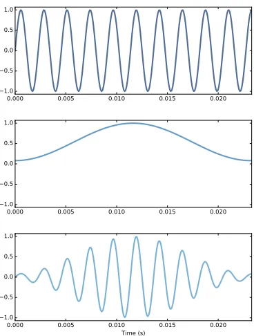
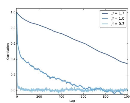
Figure 4.6 shows the resulting waveform. Like Brownian noise, it wanders up and down in a way that suggests correlation between successive values, but at least visually, it looks more random. In the next chapter we will come back to this observation and I will be more precise about what I mean by “correlation” and “more random”.

Finally, Figure 4.7 shows a spectrum for white, pink, and red noise on the same log-log scale. The relationship between the exponent,β, and the slope

of the spectrum is apparent in this figure.

4.5

Gaussian noise

(59)

4.5. Gaussian noise 47

white.

But when people talk about “white noise”, they don’t always mean UU noise. In fact, more often they mean uncorrelated Gaussian (UG) noise.

thinkdspprovides an implementation of UG noise:

class UncorrelatedGaussianNoise(_Noise):

ys = np.random.normal(0, self.amp, len(ts)) return ys

np.random.normalreturns a NumPy array of values from a Gaussian distri-bution, in this case with mean 0 and standard deviationself.amp. In theory the range of values is from negative to positive infinity, but we expect ab

Think DSP: Digital Signal Processing in Python

Think DSP

Preface

Who is this book for?

0.2. Using the code vii

Contributor List

Contents

Preface v

3 Non-periodic signals 23

Contents xi

Chapter 1

Periodic signals

1.2. Spectral decomposition 3

Spectral decomposition

1.3. Signals 5

Signals

1.4. Reading and writing Waves 7

Reading and writing Waves

Spectrums

Wave objects

1.7. Signal objects 9

Signal objects

1.8. Exercises 11

Exercises

Chapter 2

Triangle waves

2.1. Triangle waves 15

Square waves

2.3. Aliasing 17

Aliasing

2.4. Computing the spectrum 19

Computing the spectrum

2.5. Exercises 21

Exercises

Chapter 3

Linear chirp

3.1. Linear chirp 25

Exponential chirp

3.3. Spectrum of a chirp 27

Spectrum of a chirp

Spectrogram

3.5. The Gabor limit 29

The Gabor limit

Leakage

3.7. Windowing 31

Windowing

Implementing spectrograms

3.8. Implementing spectrograms 33

Exercises

3.9. Exercises 35

Chapter 4

Uncorrelated noise

switch-4.1. Uncorrelated noise 39

Integrated spectrum

4.3. Brownian noise 41

Brownian noise

4.3. Brownian noise 43

Pink Noise

4.4. Pink Noise 45

Gaussian noise

4.5. Gaussian noise 47