MoL 2018 35: Examining Personality Differences in Chit Chat Sequence to Sequence Conversational Agents

Examining Personality Differences in Chit-Chat Sequence to

Sequence Conversational Agents

MSc Thesis

(Afstudeerscriptie)

written by

Xing Yujie

(born November 8th, 1993 in Changsha, Hunan)

under the supervision of Dr Raquel Fern´andez, and submitted to the Board of Examiners in partial fulfillment of the requirements for the degree of

MSc in Logic

at the Universiteit van Amsterdam.

Date of the public defense: Members of the Thesis Committee:

July 3, 2018 Dr Tejaswini Deoskar (chair) Dr Raquel Fern´andez

Abstract

Acknowledgements

First of all, I would like to thank my supervisor Raquel Fern´andez. It is her encour-agements and supports that enable me to finish this thesis. On the practical aspect, she afforded the price of LIWC dataset for me, so that I was able to pursue the project. She gave careful and detailed comments on my thesis as well as suggestions on the project, and even corrected my typos and grammar mistakes in the thesis. She also helped me to get connected with all the people that may be helpful: she connected me with Elia Bruni, who helped me to apply for a GPU account for training models; she connected me with Tim Baumg¨artner, who helped me on PyTorch; she connected me with Sanne Bouwmeester, who helped me with the GPU cluster issues. For the mental aspect, she encouraged me many times when I was worried about the planned speed of my thesis or my future. I am very fortunate to have her as my supervisor and I have gained a lot from her, both materially and mentally.

I would like to thank my mentor Benedikt L¨owe, who helped me a lot during the period of MSc Logic. I still remember the meeting with him, where I was anxious on changing research interest from philosophy to natural language processing, while he taught me that it was natural for people to realize what they were interested in might not be what they would like to work on. Thanks to this meeting, I was able to face myself and devote myself into the new field. Also, he supported me a lot: he provided me the chance for English oral classes, and pointed me to Raquel to work on my Master Thesis. I am really lucky to have him as my mentor.

I would like to thank Evangelos Kanoulas and Kaspar Beelen for the support when I was facing the difficulty of transferring research interest. I would also like to thank Guo Jiahong and Ju Fengkui; I could not have come to ILLC without their help.

My friends also gave me encouragements and supports that mean a lot to me. Thanks all my friends in ILLC, and ILLC itself that gave me the chance to befriend with them. Thanks my friends in China, for their generous help during my difficult time, and for those pleasant chats during these years.

Contents

1 Introduction 7

1.1 Response Generation for Chit-Chat Conversational Agents . . . 8

1.1.1 Rule-Based Conversational Agents . . . 8

1.1.2 Information-Retrieval-Based Conversational Agents . . . 8

1.1.3 Generation-Based Conversational Agents . . . 9

1.2 Personality Inconsistency in Response Generation . . . 10

1.3 Overview of this Thesis . . . 11

2 Linguistic Correlates of Personality 13 2.1 Psychological Background of Personality . . . 13

2.2 Examining Personality . . . 14

2.2.1 The Big Five Personality Traits . . . 14

2.2.2 Examining OCEAN from Questionnaires . . . 15

2.2.3 Examining OCEAN Automatically . . . 16

2.2.4 Personality Recognizer . . . 17

3 Personalized Natural Language Generation 19 3.1 Natural Language Generation from Personality Features . . . 19

3.2 End-to-End Response Generation . . . 20

4 Model 24 4.1 Standard Model . . . 24

4.1.1 General Structure . . . 25

4.1.3 Attention Mechanism . . . 28

4.2 Extended Models for Personalizing . . . 29

4.2.1 Speaker Model . . . 29

4.2.2 Personality Model . . . 30

5 Experiments 32 5.1 Datasets . . . 32

5.2 Experimental Setup . . . 34

5.2.1 Training and Decoding . . . 34

5.2.2 Evaluation . . . 35

5.3 Preliminary Experiment: Examining Personality Differences for the Orig-inal Scripts . . . 37

5.4 Experiment 1: Examining Personality Differences for the Speaker Model 39 5.4.1 Experimental Procedure . . . 40

5.4.2 Results . . . 41

5.5 Experiment 2 & 3: Examining Personality Differences for the Personality Model . . . 50

5.5.1 13 Characters from the TV-series Dataset . . . 50

5.5.2 32 Extreme Personalities . . . 56

6 Conclusion 58 A Responses and OCEAN Scores 67 A.1 Responses to “Do you love me?” . . . 67

List of Tables

5.1 Characters and their respective utterance numbers . . . 34 5.2 Average overall F1 scores and accuracy scores onFriends for the original

scripts . . . 38 5.3 Statistical results onFriends for the original scripts with respect to the

baseline . . . 38 5.4 Average overall F1 scores and accuracy scores on The Big Bang Theory

for the original scripts . . . 39 5.5 Statistical results on The Big Bang Theory for the original scripts with

respect to the baseline . . . 39 5.6 Perplexity on the TV-series validation set for the standard model and

the speaker model . . . 40 5.7 Average F1 scores on the speaker model with different cleaning methods 41 5.8 Average F1 and accuracy score on Friends for the original scripts and

the speaker model . . . 42 5.9 Statistical results on Friends for the speaker model . . . 42 5.10 Average F1 scores and accuracy score on The Big Bang Theory for the

original scripts and the speaker model . . . 46 5.11 Statistical results on The Big Bang Theory for the speaker model . . . 47 5.12 Perplexity on the TV-series validation set for standard LSTM model, the

speaker model and the personality model . . . 50 5.13 Average F1 and accuracy score on Friends for the original scripts, the

5.15 Average F1 scores and accuracy score on The Big Bang Theory for the original scripts, the speaker model and the personality model . . . 54 5.16 Statistical results on The Big Bang Theory for the personality model . 54 5.17 Average Overall F1 score and accuracy score for 32 extreme personalities 56 5.18 Statistical results for 32 extreme personalities with respect to the baseline 56 A.1 Responses to Do you love me? generated by the standard model, the

speaker model and the personality model for 13 characters from the TV-series dataset . . . 68 A.2 Responses to Do you love me? generated by the personality model for

32 extreme personalities . . . 69 A.3 Average OCEAN scores for 13 characters from the TV-series dataset on

List of Figures

2.1 TIPI quesionnaire by Gosling et al. (2003) . . . 16 5.1 Gold label and predicted label onFriends for the original scripts . . . . 44 5.2 Gold label and predicted label onFriends for the speaker model . . . . 45 5.3 Gold label and predicted label onThe Big Bang Theory for the original

scripts . . . 48 5.4 Gold label and predicted label on The Big Bang Theory for the speaker

model . . . 49 5.5 Gold label and predicted label onFriends for the personality model . . 53 5.6 Gold label and predicted label onThe Big Bang Theory for the

Chapter 1

Introduction

Conversational agents, referred to as CA throughout this thesis, are those agents that serve as conversing with people. Since the first conversational agent ELIZA ( Weizen-baum,1966), there has been a long development on CA, where alongside the rule-driven method, the data-driven method has appeared. Nowadays, the data-driven method is frequently used. CA learn conversing from a big-scale dataset, thus the variety of responses is enriched.

From the perspective of the aim of CA, we can divide these agents into two cate-gories: task-oriented and non-task-oriented. Examples for task-oriented CA are chat-bots for booking restaurants or flights, where a conversation is closed once the agent has finished the task. In comparison to task-oriented CA, Non-task-oriented CA do not have tasks, or their only task is to converse. Chit-chat CA, which is the focus of this thesis, is the kind of non-task-oriented CA that are open-domain, since chit-chats are not limited to a specific domain. CA that are open-domain are more difficult to build, compared with CA with a specific domain ontology.

1.1

Response Generation for Chit-Chat

Conversa-tional Agents

There are generally three types of CA distinguished by the ways of building them: rule-based, information-retrieval-based, and generation-based.

1.1.1

Rule-Based Conversational Agents

Rule-based CA such as ELIZA have hand-written templates for answering different types of questions. The procedure is as follows: an agent first scans all the words from a question and looks for them in a keyword dictionary. If a word is found in the dictionary, the agent will select a responding template based on the question, and then fill the keyword into the selected template; if none of the words is in the dictionary, the agent returns a general response.

The limitation for this kind of CA is obvious. Although received positive feedbacks (Colby et al., 1972), due to the hand-written template and the keyword dictionary, rule-based CA have severe limitations both on the amount of possible answers and on the answering patterns; in sum, hand-written rules can only produce limited kinds of responses.

1.1.2

Information-Retrieval-Based Conversational Agents

Information-retrieval-based CA generate responses based on a big-scale corpus. The corpus often consists of human conversations; for each context-response pair in the corpus, an information-retrieval-based agent calculates the similarity between 1) the given context and the context in the pair; 2) the given context and the response in the pair. Combining 1) and 2), the agent ranks all the possible responses in the corpus and returns the top ranked one (Jurafsky and Martin, 2014).

the disadvantage is easy to see: this kind of CA are not able to generate novel responses, since all the responses come from the corpus.

1.1.3

Generation-Based Conversational Agents

Generation-based CA overcome the disadvantage of information-retrieval-based CA: instead of selecting responses from an existing corpus, a generation-based agent selects words from the vocabulary and generates responses with these words, so that it is able to generate novel responses.

The idea of generation-based CA is similar to machine translation, with the ref-erence translations in machine translation replaced by responses. For an example, an English-Chinese machine translation task takes English sentences as the source and the corresponding Chinese human reference translations as the target, while for generation-based CA, the target is replaced by the responses to the source: the English-Chinese machine translation task may take “Thank you” as the source and “谢谢” (the Chinese translation of “Thank you”) as the target, while for generation-based CA, the target will be changed to a response like “You are welcome” with respect to the source “Thank you”.

The origin of this kind of CA is from Ritter et al. (2011), where the response generation task for CA was treated as a statistical machine translation task.

In the following years, due to the development of neural networks, sequence to se-quence (Seq2Seq) model (Sutskever et al., 2014a) has been applied to the machine

translation task like Goolge Translate1 _{and gained good results (Junczys-Dowmunt}

et al., 2016). This triggered researchers to use Seq2Seq model on the response

gen-eration task (Vinyals and Le, 2015; Shang et al., 2015; Sordoni et al., 2015). Recently, researchers have proposed models that applied modifications on Seq2Seq model, or

models that combined algorithms like reinforcement learning and adversial learning with Seq2Seq model; these new models aim at making the agent generate more

spe-cific, fluent and coherent responses (Serban et al., 2016a; Li et al., 2016b, 2017b). In general, these works gained better perplexity and BLUE (Papineni et al., 2002) scores

than information-retrieval-based CA. Both perplexity (for detailed explanation, please see section 5.2.2) and BLUE are automated evaluations that measure how close to the ground-truth the predictions are; however, these scores are not suitable for evaluating the quality of generated responses (Liu et al., 2016).

Despite the success of Seq2Seqmodel on response generation, there are also

prob-lems. The agents always generate general responses such as “I don’t know”, lack consis-tency on the response content and the language style, and have difficulty in generating responses for multi-turn conversations (Zhang et al.,2018;Serban et al.,2016b). Among these problems, we are going to focus on the second one, namely the inconsistency prob-lem.

1.2

Personality Inconsistency in Response

Genera-tion

The inconsistency problem mentioned above mainly has two aspects: inconsistency of the response content and inconsistency of the language style. For example, an agent described in Li et al. (2016a) gives contradicted answers to questions that are similar in semantics but different in forms: when being asked “How old are you?”, the agent answers “16”, while when being asked “What’s your age?”, the agent answers “18”. Also, the agents lack consistent language styles, since they are trained on dataset of conversations from many different people.

Zhang et al., 2017), but these are not standard metrics. One of the works calculated the word overlapping rate among generated responses of different personalities (Zhang et al., 2017), which is able to distinguish among personalities to some extent, but is still not a suitable metric.

Since we are talking about the evaluation for personality, and personality is well studied in psychology, there are plenty of measurements we can lend from psychology. However, the concept “personality” mentioned in the above works is different from the one in psychology. In the above works, “personality” was proposed to deal with the inconsistency problem (e.g. agent claims that it is both 16 years old and 18 years old). For the two aspects of this problem: inconsistency of the response content and inconsistency of the language style, although language styles can reflect personality, the content, such as what a person likes and where he/she lives, is called external source in psychology and is not counted into “personality” in the psychological definition (Burger,

2010).

We will use the psychological definition of “personality” for this thesis, so the re-sponse content is not taken into consideration for “personality”.

1.3

Overview of this Thesis

In this thesis, we make the following contributions:

1. We provide a new evaluation method for examining the personality differences among the responses generated by personalized response generation models. 2. With the new evaluation method, we examine the speaker model proposed by Li

et al.(2016a), which we reimplement in PyTorch, if it can generate distinguished responses for different personalities as expected.

Chapter 2

Linguistic Correlates of Personality

2.1

Psychological Background of Personality

People are always different with others, yet always share similarities with others; thus, they can be classified into different types. Think of ways of classifying people: gender, age, nationality... Besides these external factors, psychologists are interested in finding a consistent factor inside individuals that can classify people’s behaviour patterns into several types; this factor is personality.

2.2

Examining Personality

The definition of personality in psychology is abstract, so psychologists have proposed many approaches of describing personality: the psychoanalytic approach, the biological approach, the humanistic approach, etc. In this thesis, we are going to use the trait approach, where personality is divided into several dimensions–the traits–that catego-rizes people with the degree to which they manifest a particular characteristic (Burger,

2010). The trait approach provides numerical description for personality, so it fits our need: automatic recognition of personality for responses.

The trait approach sees different types of personalities as consisting of traits of dif-ferent degrees. Traits are identified from data–data of personality questionnaires, data of reports of people’s daily actions, etc. For example, psychologists put the hypothesis characteristics into the questionnaire and ask subjects to answer the questionnaire; af-terwards, the psychologists analyze the results for these hypothesis characteristics, and put highly correlated ones into one cluster. Finally, each cluster will be identified as a trait.

There are several different trait schemes. For instance, the Sixteen Personality Factor Questionnaire (16 PF) by Cattell (Cattell and Mead,2008) is a famous system, where personality is broken down into 4 traits, with each trait having two poles; thus, we have 16 different types of personalities. In our thesis, instead of 16 PF, we use the Big Five Personality Traits (Norman, 1963) as the measurement for personality. We have three reasons: 1) the Big Five has consistently been found being able to capture basic dimensions of personality by multiple teams (Burger, 2010); 2) there are many works about automatic recognition on the Big Five; 3) the score of the Big Five can be treated as a numerical vector.

2.2.1

The Big Five Personality Traits

five traits. The Big Five is also called “OCEAN”, which is the combination of the initials of the five traits. The meaning of each trait is as follows:

• Extraversion measures where a person gets his/her energy from: outside him-self/herself (extravert), or inside himhim-self/herself (introvert). A person with a high score on Extraversion prefers to have more interactions with others, and is often outgoing and talkative; on the contrary, a person with low score on Extraversion prefers to stay alone, and is often quiet and reflective.

• Neuroticism measures emotional stability. A person with a high score in Neu-roticism is easier to have negative emotions such as anxiety and anger; in other words, his/her emotion is less stable. Some works use “emotional stability” in-stead of Neuroticism, where people with high scores are more emotionally stable. • Agreeableness measures people’s social agreeableness. A person with a high score is more cooperative and friendly, while a person with a low score is more competitive and suspicious.

• Conscientiousness measures how organized and responsible a person is. A person with a high score is careful and hardworking; a person with a low score is less goal-oriented and less efficient.

• Opennessmeasures people’s openness to experience. A person with a high score is more creative and curious, while a person with a low score prefers what they are familiar with to new things.

Research on OCEAN has shown that the scores of each trait is normally distributed, regardless of geographical location and cultural background (Schmitt et al., 2007).

2.2.2

Examining OCEAN from Questionnaires

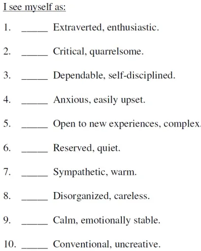
Ten Item Personality Measure (TIPI) is one of the frequently used questionnaires (Gosling et al., 2003). Subjects assess what kind of people they think they are, and express their agreements to each question using numbers: usually 1 is strongly disagree, and 7 is strongly agree. For each trait, there is a positive question and a negative question, and the score for this trait is calculated based on the answers to these two questions.

Figure 2.1: TIPI quesionnaire by Gosling et al. (2003)

2.2.3

Examining OCEAN Automatically

There are also methods for examining OCEAN automatically with language traits. Previous works have stated that OCEAN scores are correlated with linguistic features, especially the Extraversion trait. Mairesse et al. (2007) has summarized the correlated linguistic features: extraverts use more positive emotion words, and show more agree-ments and compliagree-ments than introverts (Pennebaker and King,1999); the Extraversion trait is significantly correlated with contextuality, opposed to formality (Heylighen and Dewaele, 2002); neurotics use more concrete and frequent words (Gill and Oberlander,

this topic: with a dictionary that classifies words into many categories, the researchers measured the correlation between each category and the five traits. The dictionary is the Linguistic Inquiry and Word Count (LIWC) utility.

Based on the correlation between language traits and OCEAN, researchers have proposed personality recognizer: with texts or speeches of a person, his/her personality can be automatically examined with this system.

2.2.4

Personality Recognizer

There have been some works focusing on building personality recognizer (Mairesse et al.,

2007; Oberlander and Nowson, 2006; Celli, 2012; Mohammad and Kiritchenko, 2013;

Poria et al.,2013), and most of them are classification recognizers: for example, for the Extraversion trait, the classification model predicts whether a person is an extravert or an introvert. In this thesis, we use the model of Mairesse et al. (2007), since it is the only available model, to our knowledge, that can estimate numerical scores for each trait of OCEAN, instead of binary classifications.

Below we introduce the personality recognizer of Mairesse et al. (2007) in detail.

Dataset The personality recognizer is a data-based model. The essay corpus ( Pen-nebaker and King, 1999) and EAR corpus (Mehl et al., 2006) were used as the training set. The former contains about 2500 essays annotated with OCEAN scores of the re-spective writers; the latter is a conversational corpus containing about 15000 utterances annotated with OCEAN scores of the respective speakers, and is much smaller than the former.

Structure To recognize the OCEAN score, the researchers tried several regression algorithms, such as linear regression, M5’ regression tree, and support vector machine with linear kernels. The features of the model are from LIWC (Pennebaker and King,

The loss is simply the ratio of the model’s prediction’s loss and the baseline’s loss, so that if the loss is 1, the model’s performance is equal to the baseline, while numbers less than 1 means a better performance than the baseline.

Performance For the essay corpus, almost all the ratios are lower than 1, and the estimation for Neuroticism and Openness are significantly better than the baseline. However, the best ratio is 93.58, which seems not so good. For the EAR corpus, the ratios are fluctuated, which may be caused by the relatively small scale of the dataset.

Chapter 3

Personalized Natural Language

Generation

In this chapter, we will introduce related works on personalized natural language gen-eration (NLG).

3.1

Natural Language Generation from Personality

Features

First we introduce related works on personalized NLG that generate responses from personality features. Models proposed by the works that we are going to introduce take communicative goals as input, rather than questions. To personalize the generation, parameters related to personality are also inserted into the models, together with the communicative goals.

Mairesse and Walker(2010) conducted the first research on generating distinguished utterances for different personalities. The rule-based generator they built is called Per-sonage. Personage is trianed on a restaurant dataset and it generates utterances

based on different linguistic style parameters (Mairesse et al.,2007); for example, given a high verbose parameter, it generates more words per utterance.

cor-relates the linguistic styles with OCEAN scores. Researchers asked human subjects to estimate the OCEAN score for each utterance generated based on linguistic style parameters, and trained the model with the source being the OCEAN score and the target being linguistic style parameters. The final model works as this: a person with a higher score in Extraversion trait may be more verbose, thus is predicted to have a higher verbose parameter; while a person with a lower score on Extraversion trait may express more uncertainty, thus is predicted to have a higher hedge parameter. With the predicted parameters like these, _Personage chooses responding templates corre-sponding to all of the parameters, thus is able to generate distinguished utterances for different personalities.

The latest progress for Personage is done by Oraby et al. (2018), which

pro-posed two neural generation models based on _Personage. The researchers created the training set using Personage and modified Seq2Seq TGen system (Duˇsek and

Jurˇc´ıˇcek,2016) by adding 1) dialogue acts encoded with personality information, or 2) 32 linguistic style parameters used by Personage during generating the training set.

The models they built are able to generate responses that have relatively high Pearson correlation coefficients with the training set generated by Personage.

Above works provide models that can generate distinguished utterances given dif-ferent personalities. The models are limited on the restaurant domain, and can only generate utterances for several communicative goals such as recommendation and com-parison, thus do not fit our topic on chit-chat conversations; however, the linguistic styles used for generation are also used in the personality recognizer introduced in sec-tion 2.2.4, which will be used for evaluating personality differences in our experiments. Thus, the success in generating distinguished utterances for different personalities some-how indicates the validity of the personality recognizer.

3.2

End-to-End Response Generation

systems that learn to generate responses in conversations by being exposed to large amounts of conversational data.

There are not many works that study personalized response generation; most of the works are generation-based, and the proposed models are modified from standard

Seq2Seqmodel. There is one work that is different, which applied multi-task learning

that combines a _Seq2Seq task that generates responses and an _Autoencoder task that learns embeddings of the target speaker.

Seq2Seq model consists of two parts: the encoder and the decoder, where the

encoder processes the input and forwards the result to the decoder, with which the decoder generates the outputs. For example, given a context-response pair “Thank you” and “You are welcome”, we have “Thank you” as the source to be inputted to the encoder, and “You are welcome” as the target to be inputted to the decoder. The

Seq2Seq model will be trained to generate a response that is as similar to “You are

welcome” as possible. For details, please see section 4.1.

Due to lack of conversational data with the speakers annotated, three of the works used twitter or scripts as the training set; the other two created their own corpus with volunteers making conversations for them.

Models Labeling Speaker for Each Utterance

The first and most notable work is Li et al. (2016a), where a persona-based Seq2Seq

model is proposed. They fed corresponding speaker id and addressee id together with the response sequence into the decoder, so that the model knows the speaker and addressee of each response. The persona-based model gains an improvement in both perplexity and BLUE compared to standard Seq2Seq model, and is 4.5% better in

consistency on human evaluation. Examples of generated responses of their models also show differences between different speakers.

Since existing personalized dataset is relatively small, domain adaption training is often used: aSeq2Seqmodel is first pre-trained on a big-scale conversational dataset,

(2017); the difference is that the latter trained five models separately for five speakers, which is due to lack of the structure for feeding speaker ids and addressee ids. Generally, the model proposed by the latter has same functions as the former one.

In this thesis, we also apply domain adaption training and similar models with Li et al.(2016a). The disadvantage for the persona-based model is that although it knows which utterance is spoken by whom, it has to balance between general and speaker-specific response generation, so that sometimes personalization has to be sacrificed, which will be examined in our experiment part.

Models Adding Extra Information of Speakers

There are two works that add more concrete information rather than speaker ids into the generation model. One of them isYang et al. (2017), which add speakers’ personal information such as age and gender into a Seq2Seq model. Personal information

is converted into an one-hot representation and then embedded to a dense vector, after which the vector is fed into the decoder, similar to Li et al. (2016a). The result outperforms standard Seq2Seqmodel on perplexity, BLUE and human evaluation.

The other one is the latest work by Zhang et al.(2018). They first create their own personalized corpus with volunteers; volunteers are asked to act as specific characters described by profiles no longer than five sentences, and each two of the volunteers have a conversation to know each others’ character. The researchers provide two kinds of per-sonalized model: information-retrieval-based and generation-based, and add encoded profiles into both of the models. The models both receive better human evaluations.

Model Applying Multi-Task Learning

Finally, the research by Luan et al. (2017) is different with the above works. This research applies multi-task learning: it consists of a _Seq2Seq task for generating re-sponses, and an Autoencoder task for learning the target speaker’s language style.

Both the two tasks applies _Seq2Seq model, while the _Seq2Seq task is supervised, with questions as the source and responses as the target; the Autoencoder task is

unsupervised, with the target speaker’s non-conversational sequences as both the source and the target. The parameters for the decoder are shared, which means that the model learns both general response generation and the specific language style of the target speaker. This model gains lower perplexity and higher human evaluation compared to the baseline.

This work could be seen as an extension to Li et al. (2016a) which strengthens personalization; furthermore, since the_Autoencoder task does not require conversa-tional data, the model also gives a solution to response generation for speakers who do not have enough conversational data.

Note that although the above models may generate responses distinguished in person-alities, these models are not able to generate responses given a specific personality like

Chapter 4

Model

In this chapter, we introduce the response generation models used in our experiments. First, we introduce the standard Seq2Seq model in section 4.1. After that, we

in-troduce the speaker model proposed by Li et al. (2016a). Finally, we describe the modifications we have made to build our own personality model.

4.1

Standard Model

The standard model is based on _Seq2Seq model (Sutskever et al.,2014b). Given the source sequence X =x1, x2, . . . , xm, aSeq2Seq model gives the predicted probability for a target sequence Y =y1, y2, . . . , yn with:

P(Y|X) = n

Y

t=1

P(yt|y1, . . . , yt−1, X) (4.1)

The task for the model is to improveP(Y|X) for paired ground-truthX andY, so that the target ˆY it chooses, which is of the highest probability P( ˆY|X), is preferably close toY.

We use a Seq2Seq LSTM model with attention as the standard model. Below I

4.1.1

General Structure

Our standard model–Seq2Seq LSTM model with attention–is of an encoder-decoder

structure. It takes a context sequence as the source sequenceX and a response sequence as the target sequenceY. FirstXis inputted to the encoder, and the encoder generates hidden vectors to be inserted into the decoder. Next,Y together with the hidden vectors from the encoder are inserted into the decoder, and the decoder gives predictions in the softmax layer. Attention mechanism is an extra structure to improve the model’s performance.

Encoder In each encoding step t, a word xt ∈ X is inserted to the LSTM unit for generating the corresponding hidden vector ht.

The scalar vectorxt is first embedded to a dense word-embedding vectorx∗t ∈R d×1_, where d is the number of hidden cells. Same words have same embedding vectors. Then x∗_t is inputted into the first encoding LSTM layer, together with the hidden vector h(1)_t−1 ∈ _Rd×1 _{and the cell state vector c}(1)

t−1 ∈ Rd×1 from the first layer of the previous encoding step; if t = 1, both h(1)t−1 and c

(1)

t−1 are 0 vectors. With the above inputs, the first encoding LSTM layer generates the hidden vector h(1)_t and cell state vectorc(1)_t for the current encoding step, which will be forwarded to the next layer and the next step.

Generally, each layer l > 1 generates h(l)_t and c(l)_t with 1) the hidden vector h(l−1)_t

from the previous layer; 2) the hidden vector h(l)_t−1 and the cell state vector c(l)_t−1 from the same layer of the previous step. After inputting the final word from the context sequence, we have the final hidden vectors ht (t ∈ [1,2, . . . , m]) from the final layer of each encoding steps:

H =

h

h1 h2 . . . hm

i

(4.2) H will be used in the attention mechanism, which will be explained in section4.1.3.

Similar to the encoder, for each decoding step t, we input an embedding vector

y_t∗ ∈ _Rd×1_{, which is embedded from the word y}

t ∈ Y, into the first decoding LSTM layer. Note that Y is different with X in that it always starts with EOS and ends with EOT, whereEOS notifies the model it is the end of the source and start of the target, and EOT notifies the model it is the end of the target (EOT will not be inputted into the decoder).

The hidden vector h0(1)_t−1 and the cell state vector c0(1)_t−1 from the first layer of the previous decoding step are inserted together with y_t∗. If t= 1, h0(1)_t−1 and c0(1)_t−1 are from the first layer of the final encoding step, which are h(1)m and c(1)m .

Additionally, the context vector c∗_t−1 from the previous decoding step (for details, please see section 4.1.3) is also inserted to the first decoding LSTM layer. Whilet= 1, the context vector is from the final encoding step.

With y∗_t, h0(1)_t−1, c0(1)_t−1, and c∗_t−1, the first decoding LSTM layer generates the hid-den vector h0(1)_t and cell state vector c0(1)_t for the current decoding step, which will be forwarded to the next layer and the next step. Similar to the encoder, each decoding LSTM layer l > 1 generates h0(l)_t and c0(l)_t from h0(l−1)_t , h0(l)_t−1 and c0(l)_t−1. After the final layer, a predicted vector ˆht is generated with the final hidden vector h0t and final en-coding hidden vectorsH (see section 4.1.3 for details). Then in the softmax layer, the log probabilityPt on the whole vocabulary for the next word will be predicted with ˆht:

Pt(wk) = log

exp((Ws)k·ˆht)

P

kexp((Ws)k·hˆt)

(4.3)

where wk is a word from the vocabulary V, k∈[1,|V|]; Ws ∈R|V|×d.

Training We insert the context sequence into the encoder, and the paired ground-truth response sequence into the decoder. With the log probabilities generated by the decoder for the whole vocabulary, we can get the log probability for each word of a ground-truth response, which is logP(yt|y1, . . . , yt−1, X); our goal is to minimize the sum of the log probability on all the words of ground-truth responses.

Loss(weights, B) = 1 |B|

|B|

X

b=1 nb

X

t=1

logP(yb_t|y₁b, . . . , y_t−1b , Xb) (4.4)

weights0 = weights−α∇Loss(weights, B) (4.5)

whereB is a batch of paired contexts and responses,Xb _andYb _{are paired contexts and} responses in B, and nb is the number of words in Yb. Batches are samples taken from the training set; all batches have same numbers of elements, and they do not overlap with each other. α is the learning rate; when ∇Loss(weights, B) is higher than the clipping thresholdT, α will be replaced by:

α× T

k∇Loss(weights, B)k₂ (4.6)

Decoding With the log probabilities for the next word yt on the whole vocabulary, we first transfer log probabilities into probabilities where P(yt|y1, . . . , yt−1, X)∈ [0,1], and then follow Stochastic Greedy Sampling described in Li et al.(2017a) to select the next word among the top 5 words with the highest probabilities.

4.1.2

Long Short Term Memory

Long Short Term Memory (LSTM) (Hochreiter and Schmidhuber,1997) is a solution for the gradient exploding and vanishing problem for Recurrent Neural Network. Generally, it controls how much information to keep, input and output through forget gates f, input gates i and output gates o. For each step t, given the previous hidden vector

it =σ(Wi·x∗t +Ui·ht−1) (4.7)

ft =σ(Wf ·x∗t +Uf ·ht−1) (4.8)

ot =σ(Wo·x∗t +Uo·ht−1) (4.9)

lt = tanh(Wl·xt∗ +Ul·ht−1) (4.10)

ct =ft◦ct−1+it◦lt (4.11)

ht =ot◦tanh(ct) (4.12)

where Wj, Uj ∈ Rd×d (j ∈ {i, f, o, l}). There is a slight difference for the layers l > 1,

where the input will be the hidden vector from the previous layer, which ishl−1_t , instead

x∗_t.

For the decoder, the context vector c∗_t−1 from the last step is also inputted to the first LSTM layer; so equation 4.8 changes to:

it=σ(Wi·y∗t +W c i ·c

∗

t−1+Ui·h0t−1) (4.13) where W_ic∈_Rd×d_{. Equation 4.9, 4.10, 4.11 changes in a similar way.}

4.1.3

Attention Mechanism

Attention mechanism works on the decoder, which helps the decoder to focus on lim-ited important words from the source sequence, instead of the whole source sequence (Bahdanau et al., 2014). The context vector is used both to predict probability in the softmax layer, and to be forwarded to the next step. There are different kinds of attention mechanisms, and what we apply the one from Yao et al. (2015).

vt=H>·h0t (4.14) For each encoding inputxi ∈X, we have the corresponding row of vt: vti = (H

>₎ i·h0t Then we use a softmax function to get the normalized probability of vt: at =

sof tmax(vt). For eachxi ∈X, we have:

ati =

exp(vti)

P

exp(vti)

(4.15) Combining the normalized strength indicatorat with H, we can get the context vector

c∗_t:

c∗_t =H·at (4.16)

For each j ∈ [1, d], we have c∗_t

j = Hj ·at. As mentioned in section 4.1.1 and section

4.1.2, c∗t−1 from the last step is inserted together with the embedded word y∗t ∈ Y to the current decoding step t.

Finally, for each decoding step, we combine the context vector c∗_t with the hidden vector h0_t again. The result ˆht is then sent to the softmax layer for predicting the log probability of the next word.

ˆ

ht= tanh( ˆWc∗·c_t∗+ ˆW_h·h0_t) (4.17)

where ˆWc∗,Wˆ_h ∈_Rd×d.

4.2

Extended Models for Personalizing

4.2.1

Speaker Model

The modification is on equation 4.8, 4.9, 4.10, 4.11 and is only in the first layer of LSTM decoder, similar to the modification for the context vector (see equation 4.13

in section 4.1.2). In each decoding step t, besides the embedded word, the context vector, the hidden vector and the cell state vector, which arey∗_t, c∗_t−1,ht−1 and ct−1, an embedded speaker id vector s∗ ∈_Rd×1 _{is also inputted into the model:}

it =σ(Wi·y∗t +Wic·c ∗

t−1 +Wis·s ∗

+Ui·h0t−1) (4.18) where Ws

i ∈Rd×d. Equation4.9,4.10,4.11 change in a similar way.

So each response Y is paired with the speaker’s id; like word-embedding, the same speaker id s has the same speaker-embedding vector s∗. Since every word from the same response is spoken by the same speaker, same embedded speaker id is inputted multiple times to the decoder for one response.

4.2.2

Personality Model

To address the personality differences among different speakers, and to generate differ-ent responses given differdiffer-ent personalities measured by OCEAN score, here we propose our personality model, a personality-based response generation model. Contexts are inputted as the source sequence and responses are inputted as the target sequence.

The modification is also on equation 4.8, 4.9, 4.10, 4.11 in the first layer of LSTM decoder, similar to equation4.18. The difference is that in each decoding stept, instead of inputting the embedded speaker id s∗, we input embedded OCEAN score of the speaker. We first normalized the 5-dimension OCEAN score vector OCEAN from range [1,7] to [−1,1], and then embed it with a linear layer:

OCEAN∗ =WOCEAN ·

OCEAN −4

3 (4.19)

where WOCEAN ∈Rd×5. This procedure ensures the weights of this linear layer, which

will be updated during training, is in the same scale with other weights. Next,OCEAN∗

it=σ(Wi·yt∗+W c i ·c

∗

t−1+WiOCEAN ·OCEAN ∗

+Ui ·h0t−1) (4.20) where WOCEAN

i ∈R

d×d_{. Equation4.9,4.10,4.11 change in a similar way.}

Chapter 5

Experiments

In this chapter, we introduce the three experiments we have conducted. The first ex-periment was conducted on the speaker model proposed by Li et al. (2016a), which examined personality differences on responses generated by the speaker model for char-acters from the TV-series dataset. The second and third experiments were all conducted on the personality model that we proposed; the aim of these two experiments was to test if the personality model worked as expected. The second experiment examined per-sonality differences on responses generated for characters from the TV-series dataset, and the third experiment examined personality differences on responses generated for 32 novel extreme personalities.

The structure of this chapter is as follows: In section 5.1we introduce the datasets; in section5.2we introduce the experimental setup, including the new evaluation method we propose for examining personality differences. In the later sections, we will introduce results for the three experiments one by one.

5.1

Datasets

OpenSubtitles (OSDB) Dataset The OpenSubtitles (OSDb) dataset (Tiedemann,

2009) is an open-domain dataset containing lines of movie characters. Since none of the lines is annotated with the speaker or addressee, we followed the strategy of Li et al.

context-response pair. To ensure that each utterance has enough length, we removed utterances whose length were smaller than 3. We collected 33901903 context-response pairs for the training set and 74368 pairs for the validation set. For the test set, to reduce the size of the set, we set the maximum length of a line to be 7 and removed the utterances containing more than 7 words; 2462019 context-response pairs were collected for the test set.

TV-series Dataset The TV-series dataset contains scripts of two American situation comedy TV-series: Friends1 _{andThe Big Bang Theory}2_{. Although this dataset is much} smaller than the OSDB dataset, it has each line annotated with the speaking character. However, since the addressee is not annotated, we again followed the strategy ofLi et al.

(2016a), regarding two consecutive lines as one context-response pair, first line as the context sequence and second line as the response sequence. Unlike the OSDB dataset where a context-response pair may contain utterances from different conversations, the TV-series dataset guarantees that only utterances belonging to the same scene are assigned to one pair: since the scripts of situation comedy are divided into several scenes, we are able to determine whether two utterances belong to the same scene or not. We collected 85713 pairs in total, among which about 2000 pairs for the validation set.

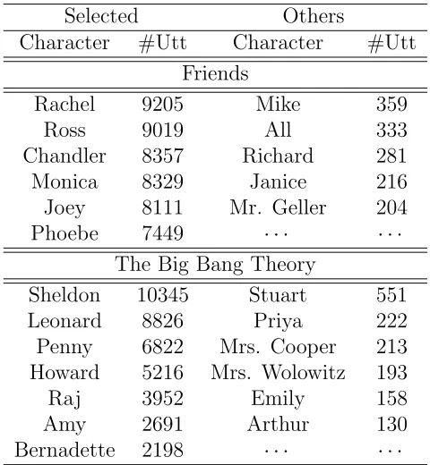
To ensure there are enough utterances during training for each character, we kept 13 characters who had more than 2000 utterances, while other characters were all labeled as “other” and were prohibited from appearing as responses. For details, please see table 5.1.

For the speaker model, we assigned each character a different speaker id. For the personality model, we annotated each of the 13 characters with his/her sample-weighed estimated OCEAN score, which was calculated as follows: for each character, we randomly selected 50 samples from his/her utterances–each sample contained 500 utterances–and estimated the OCEAN score for each sample using the personality rec-ognizer mentioned in section 2.2.4; the arithmetic mean of estimated scores for the 50

1_{https://sites.google.com/site/friendstvcorpus/}

samples was the sample-weighed estimated OCEAN score for this character.

Selected Others

Character #Utt Character #Utt Friends

Rachel 9205 Mike 359

Ross 9019 All 333

Chandler 8357 Richard 281 Monica 8329 Janice 216 Joey 8111 Mr. Geller 204 Phoebe 7449 · · · ·

The Big Bang Theory

Sheldon 10345 Stuart 551

Leonard 8826 Priya 222

Penny 6822 Mrs. Cooper 213 Howard 5216 Mrs. Wolowitz 193

Raj 3952 Emily 158

Amy 2691 Arthur 130

Bernadette 2198 · · · ·

Table 5.1: Characters and their respective utterance numbers

5.2

Experimental Setup

5.2.1

Training and Decoding

Training Since the TV-series dataset is not large enough for training, we applied the domain adaption training strategy. We first pre-trained a standard model on the larger OSDB dataset; due to the limitation of computation, we trained the model for 15 iterations on the first 1772160 pairs of the OSDB training set. The perplexity of the validation set became stable on the last iterations. Next, keeping the weights, we changed the training set from the OSDB dataset to the TV-series dataset, and trained the model for another 30 iterations, where the perplexity of the validation set of the TV-series dataset became stable for the last iterations.

with each word; for the personality model, we also fed the the speaker’s 5-dimension vector OCEAN score together with each word.

Furthermore, we used similar parameters to Li et al.(2016a) for training:

• Both the speaker model and the personality model are 4-layer LSTM models. Each layer contains 1024 hidden cells.

• We set the batch size to 128. • Vocabulary size is 25000.

• The max length for an input sentence is 50.

• Parameters are initialized with uniform distribution on [−0.1,0.1]. • Learning rate is 1.0, and it gets halved after the 6th iteration. • Threshold for clipping gradients is 5.

• Dropout rate is 0.2.

Decoding We used the test set of the OSDB dataset for decoding, which contained 2462019 contexts. We generated responses on the whole test set for each of the 13 selected characters from the TV-series dataset, both with the speaker model and the personality model. After that, we let the personality model generate responses for each of the 32 novel extreme personalities. Extreme personalities have OCEAN scores where each trait is either extremely high or extremely low; we set “extremely high” to be 6.5 and “extremely low” to be 1.5.

5.2.2

Evaluation

Perplexity

P erplexity= 1

N

p

P(wvalidation) where N is the total number of words in the validation set.

Personality Differences

We used this new evaluation method to measure if there were personality differences among the characters from the TV-series dataset for the original script, and if the speaker model and the personality model were able to generate distinguished responses for different characters or different personalities: we tried to use clustering and classi-fying algorithms to assign each OCEAN score to the correct character it belonged to, and evaluated the clustering or classifying result by the F1 score and accuracy score.

We used this method to evaluate personality differences among 1) 13 characters from the TV-series dataset; 2) 32 extreme personalities. The procedures are as follows:

Sampling For each character, we randomly selected 50 samples for clustering and 250 samples for classifying, with each sample containing 500 utterances. We then used the personality recognizer mentioned in section 2.2.4to estimate the OCEAN score for each of the 50 or 250 samples, thus we had 50 or 250 estimated OCEAN scores for one character. For each OCEAN score, we labeled it with the character it belonged to. This is the gold label.

Clustering and Classifying We tried to cluster the OCEAN scores using k-means, agglomerative and spectral clustering, and classify the OCEAN scores using neural networks and support vector machine. We will only report the results of k-means and support vector machine, since their performances are better than others. The algorithms are from scikit-learn 3,4_.

For clustering, we first clustered the OCEAN scores into several different clusters; the number of clusters was equal to the number of characters. Next, we labeled each

3_{k-means: http://scikit-learn.org/stable/modules/generated/sklearn.cluster.KMeans.html}

cluster with a different character; this predicted label maximized the purity score. Finally, we calculated the F1 score and accuracy score for the predicted label compared with the gold label.

For classifying, we applied 5-fold on the whole set: we trained the classifying model on the set 5 times, every time 80% of the set were taken as training set while the remaining 20% were the test set. We calculated the F1 score and accuracy score for the label predicted by the classifying model compared with the gold label, and then averaged the scores over 5.

Statistic Significance and Baseline We did the above procedures for 10 iterations on the original scripts (Friends and The Big Bang Theory respectively), as well as on responses generated by the speaker model and the personality model. With the F1 scores and accuracy scores for the original scripts, the speaker model and the person-ality model, we did Levene’s test and t-test to compare these scores respectively with the scores of the random baseline. The random baseline was created by randomizing the gold label in the sampling step. With Levene’s test to determine whether the population variances were equal or not, we applied independent two sample test if the population variances were equal, and Welch’s t-test if not equal.

5.3

Preliminary Experiment: Examining

Personal-ity Differences for the Original Scripts

Thus, to deal with the two worries, we first evaluated personality differences for the original scripts by calculating the F1 score and accuracy score following the above evaluation steps in section5.2.2, and comparing the results with the random baseline.

Friends

6 characters were selected from Friends. Table 5.2 shows the average overall F1 score and accuracy score over 10 iterations, and table 5.3 shows statistical analysis of F1 scores for the original scripts with respect to the baseline.

Overall Score

Algorithm Score Baseline Script k-means F1 0.228 0.470

Accuracy 0.234 0.478 SVM F1 0.164 0.606 Accuracy 0.169 0.610

Table 5.2: Average overall F1 scores and accuracy scores on Friends for the original scripts

p-value Cohen’s d k-means 3.03×10−15∗∗ 10.9

SVM 1.22×10−23∗∗ 32.3

Table 5.3: Statistical results on Friends for the original scripts with respect to the baseline

Scores higher than 0.5 are colored red. Remember that the baseline is created by replacing the gold label with the random label; thus, if the estimated OCEAN scores for each character are not distinguished from other characters, the overall F1 score and accuracy score should not be significantly different from the baseline. However, both the overall F1 score and accuracy score for the original scripts are higher than the baseline significantly, which indicates that the OCEAN scores estimated for each character for the original scripts are distinguished with those for other characters.

the original scripts for different characters are able to reflect distinguished personalities to some extent.

The Big Bang Theory

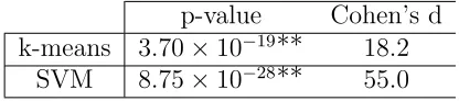
7 characters were selected from The Big Bang Theory. Table 5.4 shows the average overall F1 score and accuracy score over 10 iterations, and table 5.5 shows statistical analysis of F1 scores for the original scripts with respect to the baseline.

Overall Score

Algorithm Score Baseline Script k-means F1 0.208 0.621

Accuracy 0.210 0.625

SVM F1 0.140 0.683 Accuracy 0.144 0.690

Table 5.4: Average overall F1 scores and accuracy scores on The Big Bang Theory for the original scripts

p-value Cohen’s d k-means 3.70×10−19∗∗ 18.2

SVM 8.75×10−28∗∗ 55.0

Table 5.5: Statistical results on The Big Bang Theory for the original scripts with respect to the baseline

Scores higher than 0.5 are colored red. The result is even better thanFriends, so we can again infer that: 1) the personality recognizer works well; 2) the original scripts for different characters are able to reflect distinguished personalities to some extent; 3) the original scripts for each character from The Big Bang Theory are more distinguished than those fromFriends.

5.4

Experiment 1: Examining Personality

Differ-ences for the Speaker Model

Standard Model the speaker model Perplexity 40.68 38.78

Table 5.6: Perplexity on the TV-series validation set for the standard model and the speaker model

Although there is a decrease on perplexity for the speaker model compared to the standard model, the difference is not so significant as reported in Li et al. (2016a). This may be caused by the small size of the TV-series dataset, or reducing of the OSDB dataset in section 5.2.1.

5.4.1

Experimental Procedure

The first step of this experiment is to generate responses for each character; we let the speaker model generate responses for each of the 13 characters using the OSDB test set as inputs, as mentioned in section 5.2.1 (for examples of generated responses, see appendix A.1). After that, we did a second step: cleaning the generated responses by removing the general responses.

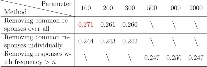
The generated responses have a lot of general responses such as “I know”. Since the general responses are the same for each character, it is likely that the samples for different characters are all filled with general responses, which makes it impossible for examining personality differences. To get rid of the general responses, we tried 3 meth-ods with different parameters, which are: 1) removing the n top common responses over all characters; 2) removing then top common responses individually for each char-acter; 3) removing all responses with frequency higher than n in any single character’s responses.

For each of these methods, we first cleaned the responses using this method, and then went through the first two steps of examining personality differences, including

sampling and clustering. For selecting these parameters, we did clustering on all of the 13 characters using k-means, and calculated the average overall F1 scores. The result is shown in table 5.7.

Method

Parameter

100 200 300 500 1000 2000 Removing common

re-0.271 0.261 0.260

\

\

\

Removing common

re-0.244 0.243 0.242

\

\

\

Removing responses

w-\

\

\

Table 5.7: Average F1 scores on the speaker model with different cleaning methods

responses left for each character.

Next, we followed the steps mentioned in section 5.2.2 for evaluating personality differences. We sampled and estimated OCEAN scores for the cleaned responses, and then clustered & classified these OCEAN scores (for estimated OCEAN scores, see appendix A.2). For this step, we selected the clustering & classifying algorithms that gave best scores, which are k-means for clustering and support vector machine for classifying. We applied model selection on both of the two algorithms. For classifying, we have two options: 1) train separate classification models on the original scripts and on the speaker model; 2) train the classification model on the original scripts, and use it to do classifications on the speaker model. We tried both of the two options; in the result part, 1) will be referred as SVM, and 2) will be referred as SVM*.

Finally we calculated F1 scores and accuracy scores on the clustering & classify-ing results for 10 iterations, and compared the scores for the original scripts and the baseline.

5.4.2

Results

Friends

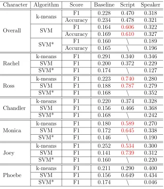
Same as the original scripts, 6 characters were selected from Friends. Table 5.8 shows the average F1 scores and accuracy scores over 10 iterations, and table 5.9 shows sta-tistical analysis of F1 scores for the speaker model, with respect to the baseline and the original scripts.

Character Algorithm Score Baseline Script Speaker

Overall

k-means F1 0.228 0.470 0.318 Accuracy 0.234 0.478 0.321 SVM F1 0.164 0.606 0.322 Accuracy 0.169 0.610 0.327

SVM* F1 0.160 \ 0.189

Accuracy 0.165 \ 0.196 Rachel

k-means F1 0.291 0.340 0.346 SVM F1 0.200 0.372 0.229

SVM* F1 0.174 \ 0.127

Ross

k-means F1 0.223 0.740 0.280 SVM F1 0.188 0.787 0.279

SVM* F1 0.168 \ 0.352

Chandler

k-means F1 0.220 0.374 0.328 SVM F1 0.156 0.466 0.368

SVM* F1 0.168 \ 0.242

Monica

k-means F1 0.180 0.589 0.270 SVM F1 0.172 0.645 0.338

SVM* F1 0.146 \ 0.190

Joey

k-means F1 0.252 0.534 0.300 SVM F1 0.141 0.739 0.312

SVM* F1 0.160 \ 0.220

Phoebe

k-means F1 0.211 0.290 0.400 SVM F1 0.156 0.649 0.434

SVM* F1 0.174 \ 0.046

Table 5.8: Average F1 and accuracy score on Friends for the original scripts and the speaker model

Baseline Script

the speaker model

k-means p-value 6.23×10

−10∗∗ _6.08×10−11∗∗ Cohen’s d 5.30 6.11 SVM p-value 2.87×10

−18∗∗ _9.60×10−20∗∗ Cohen’s d 16.2 19.6 SVM* p-value 4.44×10

−5∗∗ _3.12×10−22∗∗ Cohen’s d 2.39 27.0 Table 5.9: Statistical results onFriends for the speaker model

infer that the speaker model is able to generate responses that are distinguished in personality.

Moreover, from table 5.8 and 5.9, we can see that although the overall F1 score for the original scripts and the speaker model are all significantly higher than the baseline, the speaker model has a significantly worse score than the original scripts. This indicates that the responses for different characters generated by the speaker model are less distinguished than the original scripts. This may be caused by 1) the influence of general responses that have not been totally cleaned; 2) that the original scripts are not distinguished enough for different characters, so that the speaker model, which takes the original scripts as the training set, is not able to learn the differences very well.

Finally, note that for SVM*, the classification model is trained on the original scripts while predicts classifications for responses generated by the speaker model. This method examines if the OCEAN score estimated for a specific character whose responses are generated by the speaker model, is similar to the OCEAN score estimated for this character based on the original scripts. That is to say, whether the speaker model can generate tailor-made responses for this specific character or not. The scores are higher than the baseline significantly, which means that the speaker model captured some nature of the personality estimated for each character, however not much, since the effect size is low (Cohen’s d= 2.39) over all characters. Also the scores for SVM* is lower than SVM, which means that although the speaker model can generate distinguished responses for different characters, these responses are not exactly tailor-made for those characters. The reasons may be that 1) the TV-series dataset is relatively small; 2) the estimations of OCEAN scores for the characters are not so precise.

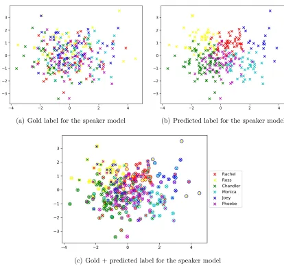
Several figures follow the table, which are visualization of the clustering results, with data decomposed by PCA into 2 dimensions. Figure5.1shows the predicted label of the 6 characters for the original scripts, and the differences between the predicted label and the gold label. Each character has 50 samples. Similarly, figure5.2 shows the predicted label for the speaker model and its differences with the gold label.

(a) Gold label for the original scripts (b) Predicted label for the original scripts

(c) Gold + predicted label for the original scripts

Figure 5.1: Gold label and predicted label on Friends for the original scripts

Figure 5.1(c) and 5.2(c) combine the predicted label with the gold label: the crosses are the gold label, while the circles are the predicted label. Thus, more messy the color, worse the performance. Due to the composition of dimension, the figures are not able to show all the details.

(a) Gold label for the speaker model (b) Predicted label for the speaker model

(c) Gold + predicted label for the speaker model

Figure 5.2: Gold label and predicted label on Friends for the speaker model

is a visualization of the result of SVM*.

The Big Bang Theory

Same as the original scripts, 7 characters were selected from The Big Bang Theory. Table5.10 shows the average F1 scores and accuracy score over 10 iterations, and table

5.11 shows statistical analysis of F1 scores for the speaker model with respect to the baseline and the original scripts.

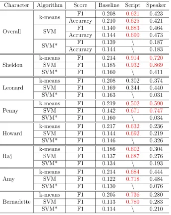
Character Algorithm Score Baseline Script Speaker

Overall

k-means F1 0.208 0.621 0.423 Accuracy 0.210 0.625 0.421 SVM F1 0.140 0.683 0.464 Accuracy 0.144 0.690 0.473

SVM* F1 0.139 \ 0.187

Accuracy 0.144 \ 0.183 Sheldon

k-means F1 0.214 0.914 0.720

SVM F1 0.185 0.932 0.869

SVM* F1 0.160 \ 0.411

Leonard

k-means F1 0.208 0.302 0.374 SVM F1 0.169 0.344 0.440

SVM* F1 0.163 \ 0.031

Penny

k-means F1 0.219 0.502 0.590

SVM F1 0.142 0.671 0.747

SVM* F1 0.160 \ 0.034

Howard

k-means F1 0.217 0.632 0.236 SVM F1 0.144 0.692 0.219

SVM* F1 0.146 \ 0.326

Raj

k-means F1 0.186 0.602 0.304 SVM F1 0.137 0.687 0.276

SVM* F1 0.134 \ 0.193

Amy

k-means F1 0.214 0.684 0.444 SVM F1 0.122 0.718 0.484

SVM* F1 0.130 \ 0.076

Bernadette

k-means F1 0.205 0.736 0.280 SVM F1 0.113 0.780 0.283

SVM* F1 0.114 \ 0.210

Table 5.10: Average F1 scores and accuracy score on The Big Bang Theory for the original scripts and the speaker model

Baseline Script

the speaker model

k-means p-value 2.45×10

−19∗∗ _1.55×10−13∗∗ Cohen’s d 18.6 8.70 SVM p-value 3.70×10

−24∗∗ _5.92×10−20∗∗ Cohen’s d 34.6 20.1 SVM* p-value 1.15×10

−7∗∗ _3.42×10−24∗∗ Cohen’s d 3.77 34.7

Table 5.11: Statistical results on The Big Bang Theory for the speaker model

responses for different characters generated by the speaker model are less distinguished than the original scripts.

Moreover, it can be observed from table5.10that the overall F1 score and accuracy score for the original scripts and the speaker model onThe Big Bang Theory is higher than Friends, while the baseline is lower than Friends. Lower score for the baseline is due to the increasing of characters: 7 characters for The Big Bang Theory and 6 characters for Friends. The scores under SVM* for the speaker model is similar to Friends, yet due to the lower baseline, the scores are actually better thanFriends.

The reason for a higher overall score compared to Friends is that 1) the original scripts are more distinguished among all characters: 6 out of 7 characters have F1 scores higher than 0.5 for the original scripts, while this number on Friends is 3 out of 6; 2) there is a highly distinguished character, which results in the improvement of the overall score. With the more distinguished original scripts as the training set, the speaker model may learn better on the differences between characters, thus generate more distinguished responses for each character.

It is notable that the character “Sheldon” gained a very high F1 score for the speaker model, from which we can infer that the speaker model can capture the nature of a character, if the corresponding original scripts are distinguished enough, which can be measured by the F1 score and accuracy score.

(a) Gold label for the original scripts (b) Predicted label for the original scripts

(c) Gold + predicted label for the original scripts

Figure 5.3: Gold label and predicted label on The Big Bang Theory for the original scripts

predicted label for the speaker model and its difference with the gold label.

(a) Gold label for the speaker model (b) Predicted label for the speaker model

(c) Gold + predicted label for the speaker model

Figure 5.4: Gold label and predicted label on The Big Bang Theory for the speaker model

generated responses have similar OCEAN scores with the original scripts, which is same to the result of SVM* in table5.10.

5.5

Experiment 2 & 3: Examining Personality

Dif-ferences for the Personality Model

5.5.1

13 Characters from the TV-series Dataset

We examined if the responses generated by the personality model for 13 characters from TV-series dataset reflected personality differences. First we show the perplexity of the personality model:

Standard LSTM the speaker model the personality model

Perplexity 40.68 38.78 38.63

Table 5.12: Perplexity on the TV-series validation set for standard LSTM model, the speaker model and the personality model

The personality model has a lower perplexity than the speaker model, but the difference is not significant.

The experimental procedures for this experiment is similar to experiment 1 (for examples of generated responses and estimated OCEAN scores, see appendix A.1 and

A.2). It may worth noting that we also cleaned the generated responses by removing the top 100 common responses over all characters.

Friends

Same as the speaker model, 6 characters were selected fromFriends. Table 5.13 shows the average F1 scores and accuracy scores over 10 iterations, which is similar to table

5.8in experiment 1, but different at that there is an extra column for personality scores. Table5.14 shows statistical analysis of F1 scores for the personality model with respect to the baseline, the original scripts, and the speaker model.

Character Algorithm Score Baseline Script Speaker Personality

Overall

k-means F1 0.228 0.470 0.318 0.265 Accuracy 0.234 0.478 0.321 0.268 SVM F1 0.164 0.606 0.322 0.214 Accuracy 0.169 0.610 0.327 0.221 SVM* F1 0.160 \ 0.189 0.185 Accuracy 0.165 \ 0.196 0.204 Rachel

k-means F1 0.291 0.340 0.346 0.240 SVM F1 0.200 0.372 0.229 0.188 SVM* F1 0.174 \ 0.127 0.147 Ross

k-means F1 0.223 0.740 0.280 0.326 SVM F1 0.188 0.787 0.279 0.386 SVM* F1 0.168 \ 0.352 0.472 Chandler

k-means F1 0.220 0.374 0.328 0.263 SVM F1 0.156 0.466 0.368 0.195 SVM* F1 0.168 \ 0.242 0.221 Monica

k-means F1 0.180 0.589 0.270 0.260 SVM F1 0.172 0.645 0.338 0.257 SVM* F1 0.146 \ 0.190 0.235 Joey

k-means F1 0.252 0.534 0.300 0.280 SVM F1 0.141 0.739 0.312 0.152 SVM* F1 0.160 \ 0.220 0.094 Phoebe

k-means F1 0.211 0.290 0.400 0.232 SVM F1 0.156 0.649 0.434 0.150 SVM* F1 0.174 \ 0.046 0.054

Table 5.13: Average F1 and accuracy score on Friends for the original scripts, the speaker model and the personality model

Baseline Script Speaker

the per-sonality model

k-means p-value 2.48×10

−5∗∗ _1.52×10−13∗∗ _6.15×10−6∗∗ Cohen’s d 2.51 8.71 2.82 SVM p-value 1.09×10

−7∗∗ _5.02×10−21∗∗ _1.23×10−12∗∗ Cohen’s d 3.79 23.1 7.71 SVM* p-value 1.14×10

−6∗∗ _1.55×10−22∗∗ _0.19 Cohen’s d 3.20 28.1 0.339 Table 5.14: Statistical results onFriends for the personality model

responses that are distinguished in personality.