A Kernel-Based Two-Class Classifier
for Imbalanced Data Sets
Xia Hong
, Senior Member, IEEE
, Sheng Chen
, Senior Member, IEEE
, and Chris J. Harris
Abstract—Many kernel classifier construction algorithms adopt classification accuracy as performance metrics in model evalu-ation. Moreover, equal weighting is often applied to each data sample in parameter estimation. These modeling practices often become problematic if the data sets are imbalanced. We present a kernel classifier construction algorithm using orthogonal forward selection (OFS) in order to optimize the model generalization for imbalanced two-class data sets. This kernel classifier identification algorithm is based on a new regularized orthogonal weighted least squares (ROWLS) estimator and the model selection crite-rion of maximal leave-one-out area under curve (LOO-AUC) of the receiver operating characteristics (ROCs). It is shown that, owing to the orthogonalization procedure, the LOO-AUC can be calculated via an analytic formula based on the new regularized orthogonal weighted least squares parameter estimator, without actually splitting the estimation data set. The proposed algorithm can achieve minimal computational expense via a set of forward recursive updating formula in searching model terms with max-imal incremental LOO-AUC value. Numerical examples are used to demonstrate the efficacy of the algorithm.
Index Terms—Forward selection, imbalanced data sets, kernel classifier, leave-one-out (LOO) cross validation, receiver operating characteristics (ROCs).
I. INTRODUCTION
M
ODEL EVALUATION in terms of good generalization performance is essential in the development and analysis of data-based learning algorithms for the construction of object classifiers. A fundamental concept in the evaluation of model generalization capability is that of cross validation [1], e.g., leave-one-out (LOO) cross validation is often used to estimate generalization error by choosing amongst different network architectures [1]. The study of classifiers for improving model generalization capability has been widely researched [2]–[10]. In most model combinatory approaches, it is assumed that a set of different classifiers with some reasonable performances are readily available. Cross validation, as required in most algo-rithms for model generalization evaluation, contributes signifi-cantly to computational cost. Clearly, the overall computational cost is intensive for most model combinatory approaches. Al-ternatively, in order to produce an individual model with good generalization for regression/classification, there has beensig-Manuscript received July 7, 2005; revised June 12, 2006. This work was sup-ported in part by the U.K. Engineering and Physical Sciences Research Council (EPSRC).
X. Hong is with the Cybernetic Intelligence Research Group, School of Sys-tems Engineering, University of Reading, Reading RG6 6AY, U.K. (e-mail: [email protected]).
S. Chen and C. J. Harris are with the School of Electronics and Computer Science, University of Southampton, Southampton SO17 1BJ, U.K.
Digital Object Identifier 10.1109/TNN.2006.882812
nificant research on kernel-model-based construction/selection approached, such as support vector machine (SVM), relevance vector machine (RVM), and orthogonal forward regression (OFR), etc., [11]–[14]. The efficient construction of a sparse model representation is crucial in generating a model that is easy to use and generalizes well. A class of forward orthogonal least squares (OLS) algorithms to select model regressors in a forward regression manner by virtue of their contributions to the model, which are measured by some objective function for model construction, have been developed [14]–[19]. For the construction of a sparse regression model that generalizes well, regressors are incrementally appended in an efficient forward regression procedure while minimizing the LOO errors [18], [19]. For the two-class classification problem, sparse kernel classifiers can be constructed via incrementally maximizing the Fisher ratio of class separability using the orthogonal forward selection (OFS) procedure [20], [21]. Alternatively, the data-structure-preserving criterion has been introduced as a neuron selection criterion to improve model generalization [22]. Recent work [23] has developed an OFS procedure based on minimizing the LOO misclassification rate for constructing a two-class classifier. It has been shown in [18], [19], and [23] that LOO cross validation for good model generalization can be performed efficiently, without resort to either actually splitting the estimation data set or utilizing an additional validation data set due to orthogonalization decomposition used in forward selection.
Many techniques on classifier construction, including kernel classifier of standard SVM, RVM, or OFS, are based on clas-sification accuracy as a performance metric. This type of per-formance metric may break down if the class distribution is not well balanced, or if the two types of misclassification costs are skewed [9], [24]. A common problem in learning the imbal-anced data sets using classification accuracy as modeling objec-tive function is that a trained classifier tends to classify all ex-amples to the major class [25]. Boosting algorithms have been developed [25], [26] based on the optimal setting of the margin given by imbalanced data sets, in which the parameter estimator uses unequal weights for data samples based on their margins. There has been considerable interest in cost-sensitive classifi-cation [9], [25]–[27]. An essential characteristic of cost-sensi-tive classifiers is that they can successfully handle imbalanced data and/or skewed misclassification cost. In [27], the cost is defined as a general performance metric including the costs of misclassification errors and experiments. In the context of SVM kernel classifiers, techniques have been introduced for imbal-anced training data sets including a control sensitivity loss func-tion [28], a kernel boundary alignment (KBA) algorithm [29],
and a proximal SVM algorithm [30]. A novel concept of using autoassociator neural network to be trained only by one partic-ular class data samples has been proposed by Japkowicz [31]. The associator is applied to new data samples by comparing its reconstruction error to a threshold. In the context of -nearest neighbor classifiers [2], a neighbor-weighted -nearest neighbor (NKKNN) algorithm has been introduced and applied to im-balanced text categorization [32]. A theoretically sophisticated model combinatory approach known as random forest (RF) is shown to be the most accurate classifier for many benchmark data sets [5]. One remarkable feature of the RF is that it does not overfit since its generalization error converges asymptoti-cally to a limit as the number of trees in the forest becomes large. There are other valuable original approaches developed for learning from imbalanced data sets through sampling tech-niques [33], [34]. The techtech-niques of cost-sensitive learning and sampling has been introduced in an RF classifier for imbalanced data sets [35] with superior classification performance.
Fundamental to the modeling of imbalanced data sets is the receiver operating characteristics (ROCs) which is a classical methodology from signal detection theory [36], [37]. The ROC analysis has been widely used in medical diagnosis [37] and is receiving considerable attention in the machine learning re-search community [9]. It has been shown that the ROC ap-proach is a powerful tool both for making practical choices and for drawing scientific conclusions [24]. The cost of misclas-sification is described in [9], in which the ROC convex hull (ROCCH) method has been introduced to manage (via com-bining or voting) classifiers. One of the performance metrics used in the ROC analysis [9], [36], [37] is to maximize the area under curve (AUC) of an ROC, which is equivalent to the prob-ability that for a pair of randomly drawn data samples from the positive and negative groups respectively, the classifier ranks the positive sample higher than the negative sample in terms of “being positive.”
In all the aforementioned OLS or OFS algorithms [14]–[21], [23], the model parameters are based on a least squares or a regularized lease squares estimator, with equal weighting for all data points in estimation. Intuitively, this type of estimator, if used for imbalanced data, will produce unfavorable classifi-cation results for the minority class. As the forward selection model construction algorithms are computationally efficient al-gorithms in producing parsimonious kernel models, it is then desirable to develop new forward selection model construction algorithms for building two-class classifiers from imbalanced data sets, and this is the objective of this paper. Note that in for-ward-orthogonal-selection-based algorithms, two cost functions are generally utilized. These are as follows: 1) a parameter esti-mation cost function which is used to derive parameters for can-didate models, such as least squares parameter estimators; and 2) model selective criteria, which are used to decide amongst the candidate models, i.e., which term to be included into the model in each forward regression step. From previous analysis, it is seen that there are two feasible approaches in order to iden-tify a classifier suitable for imbalanced data sets: i) for model performance criteria, the criteria as in ROC analysis are prefer-able to classification accuracy as model selective criteria; and
ii) for parameter estimators, applying unequal weighting factors for data points instead of equal weighting as used in most least squares solutions in forward regression algorithms.
Consequently, we derive the proposed algorithm containing two elements specifically for effectively handling imbalanced data sets. First, by combining the concepts of LOO cross val-idation and AUC, the model generalization metrics via leave-one-out area under curve (LOO-AUC) is used as the objec-tive function to select the model kernels in a forward selec-tion manner. For a two-class classificaselec-tion problem with imbal-anced data samples, and/or imbalimbal-anced misclassification cost, it is helpful to build up a parameter estimator using some cost function that is sensitive to the data sample’s importance for classification [25], [26]. Another element of this paper is to introduce a new forward regression model structure selection algorithm, the forward regularized orthogonal weighted least squares algorithm (FROWLS), in which the parameter estima-tion cost funcestima-tion is sensitive to their class labels, i.e., by as-signing more weights on the error due to a data sample in the minority class, but less weights on the error due to a data sample in the majority class.
This paper is organized as follows. Section II initially intro-duces the ROC plane and LOO-AUC which forms the basic idea of model generalization evaluation for imbalanced data sets. Section III introduces the new kernel classifier identifi-cation algorithm for imbalanced data sets, by using forward selection algorithm based on a new regularized orthogonal weighted least squares algorithm as parameter estimator and a maximal LOO-AUC as model selective criterion. It is shown that LOO-AUC can be calculated via analytic formula based on a new regularized orthogonal weighted least squares algo-rithm as a parameter estimator, rather that actually splitting the estimation data set owing to orthogonalization procedure. The proposed algorithm can achieve minimal computational expense via a set of forward recursive updating formulas in the search of terms with maximal LOO-AUC. Finally, the proposed two-class kernel classifier construction algorithm is presented using OFS by directly maximizing the LOO-AUC in order to optimize the model generalization for imbalanced data sets. Numerical examples are used to demonstrate the efficacy of the algorithm in Section IV and conclusions are given in Section V.
II. ROC PLANE ANDAUC
Consider a data set consisting of -dimensional data samples that belong to a two-class set,
i.e., , where is used to
TABLE I
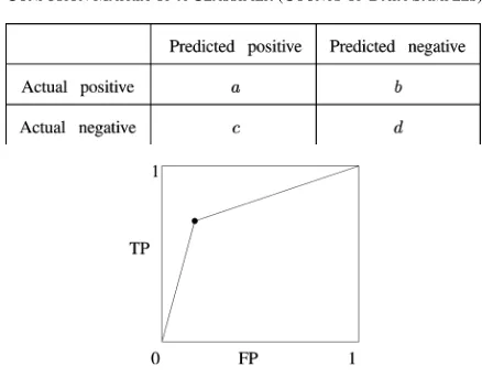
[image:3.594.54.273.86.257.2]CONFUSIONMATRIX OF ACLASSIFIER(COUNTS OFDATASAMPLES)
Fig. 1. ROC of a single classifier.
Clearly and . The true positive rate (TP) is the proportion of positive data samples that were correctly identified, as given by [37]
TP (1)
The false positive rate (FP) is the proportion of the negatives data samples that were incorrectly classified as positive, as cal-culated using [37]
FP (2)
Note that maximizing classification accuracy (CA) of
CA (3)
is a commonly used performance metric, which is equivalent to minimizing the misclassification rate of the classifier.
Alternatively, a classifier can be mapped as a point in two-di-mensional (2-D) ROC plane with coordinates as {FP, TP}, as shown in Fig. 1. By connecting this point with and , we get the ROC curve for a nonprobabilistic or hard classifier. ROC analysis is commonly applied in visualizing model per-formance, decision analysis, and model combinations [9] with extensive scope and applications [36], [37]. The ROC is a graph showing the conditional probability of classifying positive sam-ples as positive plotted against the conditional probability of classifying negative samples as positive [37]. From left to right, the ROC represents the variation of performance of the classi-fier if the criterion of choosing positive becomes more lenient. The ROC curve shows the tradeoff between TP and FP that ac-knowledges the fact that the capacity of any classifier cannot in-crease TP without also increasing FP. The area under the ROC curve AUC is one of the performance metrics in the ROC anal-ysis [9], [36], [37], which is equivalent to the probability that, given a pair of randomly drawn data samples from the positive and negative groups, respectively, the classifier ranks the posi-tive sample higher than the negaposi-tive sample in terms of “being positive.” Note that an AUC of 0.50 means that the diagnostic
accuracy is equivalent to a pure random guess, and an AUC of 1 means that the classier distinguishes class examples perfectly. One way of selecting classifier is based on using a classifier which maximizes the AUC of a ROC, which can be calculated by
AUC TP FP (4)
for the ROC curve of a single hard classifier as shown in Fig. 1. Equation (4) can be easily adjusted to cope with cost-sensi-tive classification if the misclassification costs are skewed [9], or other performance metrics derived from TP and FP are used. Clearly, the AUC of (4) is a classifier metric with a tradeoff be-tween high TP and low FP. Note that if the data set is completely balanced with , then AUC CA [see (3)]. However, for imbalanced data sets, this equivalence no longer holds. By separating the performance of a classifier into two terms that represent the performance for two classes, respectively, in com-parison to the classification accuracy of (3) which only has a single term, this enables the possibility to manage the classifi-cation performance for imbalanced data.
Alternatively, cross-validation criteria are metrics that mea-sure model’s generalization capability [1]. One commonly used version of a cross validation is the LOO cross validation. The idea is that, for a given classifier model structure, each data point in the estimation data set is sequentially set aside in turn, a classifier is estimated using the remaining data, and the predicted label is derived for the data point that was removed. By excluding the th data example in estimation data set, the output of the model for the th data example using a model es-timated by using remaining data examples is denoted as , or in short . We can use the LOO-AUC as the metrics for model generalization in terms of AUC perfor-mance, as calculated by
AUC TP FP (5)
where TP
FP (6)
in which the indicator functions for TP and for FP are defined as
if and otherwise if and otherwise.
set. Consequently, we achieve good model generalization per-formance without resort to an additional validation data set. In Section III, a new forward orthogonal weighted least squares (FOWLS) classifier construction algorithm is introduced based on the model selective criterion of maximizing LOO-AUC given by (5), in which a set of forward recursive updating formula for fast calculation of LOO-AUC is developed based on the kernel classifier model representation in orthogonal form.
III. FROWLSFORCLASSIFIERCONSTRUCTION
Consider the kernel classifier
with (7)
where denotes the classifier kernels. is the number of kernels and is the estimated class label for . ,
denotes the classifier weights. The Gaussian kernel
functions are used in
this paper, where the centers ’s are to be selected from the full set of input vectors as a subset, and is the width parameter assumed to be appropriately chosen by the user.
Given the training data set , define
the kernel matrix in which
. Over the training data set, (7) can be written in vector form as
(8)
where , and
is model residual vector with
. is the classifier’s weight vector. is the classifier output vector. Geometrically, a set of weight vectors of the kernel model defines a hyperplane of
(9)
dividing the data into two classes.
The LOO predicted label of a kernel classifier of (7),
is given by , in which is the
model prediction evaluated using the th data sample, from a model estimated from the data set , i.e., the th data sample is removed from for estimation. By definition, we have and
, so that
TP
FP (10)
with .
The basic idea in the proposed algorithm is that the efficient evaluation of LOO-AUC can be achieved through the fast cal-culation of . In the following, it will be shown that the cal-culation of can be performed efficiently without actually
splitting the training data set. An analytic formula of is given in Section III-B, based on a new regularized orthogonal weighted least squares (ROWLS) classifier estimator as intro-duced in Section III-A.
A. ROWLS Parameter Estimation
For a two-class problem, sparse kernel classifiers can be con-structed using the OFS procedure [20], [21], [23]. A common feature of these algorithms is that least squares type parameter estimators have been used for parameter estimation. Note that parameter estimators that directly optimize classification perfor-mance are generally difficult to find due to the factors such as unknown probability function of the data distribution, or pos-sibly nondifferentiable objective functions. The advantage of using a least-squares-type parameter estimator is that the clas-sifier can be easily obtained, but the disadvantage is that they are not directly derived by optimizing the results of classifica-tion, or the cost of classification. The OFS procedure [20], [21], [23] can effectively alleviate this disadvantage as we initially use least squares type parameter estimator for generating can-didate models, followed by direct evaluation of these models in terms of classification performance, i.e., minimizing the LOO misclassification rate [23]. The model selection step can, there-fore, guarantee that the best model in terms of classification per-formance is found amongst the candidate models.
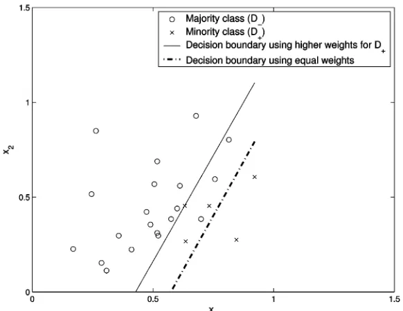
A common scenario in learning the imbalanced data sets is that the trained classifier tends to classify all examples to the major class [25]. In practice, it is often very important to have accurate classification for the minority class, e.g., in the appli-cation of abnormality detection. For this purpose, in the pro-posed algorithm, the maximization of LOO-AUC is used as the model selection criterion to choose from candidate models. However, in order to guarantee that the final model has a high value of LOO-AUC, it is necessary to make sure that the pa-rameter estimation for candidate models is appropriate for im-balanced data. Intuitively, for imim-balanced data, least squares or regularized lease squares estimator with equal weighting for all data points will produce unfavorable classification results for the minority class, which has a much smaller influence than the ma-jority class to the resultant parameter estimates, and hence the decision boundary. A basic idea is that it is helpful to build up a parameter estimator using some cost function that is sensitive to data sample’s importance for classification [25], [26] in order to produce better candidate models. In this paper, the parameter estimator is based on the following cost function:
(11)
Fig. 2. Effect of using (11) as a cost function; here, a linear discriminant function is used for illustration.
Let , in which
if if
Then, (11) can be expressed in vector form
(12) in which the equation shown at the bottom of the page holds, and the nonsingular square root matrix of is denoted by
.
Denote . The column and row vectors of
are represented by , and
, respectively. Let an orthogonal decompo-sition of be , where is an upper tri-angular matrix. is a matrix with orthogonal columns that satisfy
(13)
with
(14)
The column and row vectors of are represented by
, and ,
respec-tively. The aforementioned orthogonal decomposition can be realized through the Gram–Schmidt procedure by transferring nonorthogonal vectors , to orthogonal vectors
, . Note that
(15) where is a weight vector in orthog-onal space. Equation (15) is equivalent to
(16)
The ROWLS parameter estimator is the parameter vector that minimizes the cost function , where is the regularization parameter as set by the user
(17) By setting , ’s are obtained as
(18)
B. Analytic Formula for Evaluating
Based on the regularized orthogonal least squares model pa-rameters given by (18), the model residuals can be represented by
(19)
The LOO model residual is given by
(20)
It has been shown [19] that for regularized orthogonal least squares estimator, the LOO model residuals can be derived using an algebraic operation rather than actually splitting the training data set based on the Sherman–Morrison–Woodbury theorem [38]. For models evaluated using regularized orthog-onal weighted least square parameter estimates, it can be shown that the LOO model residuals are given by (see Appendix)
(21)
which has the same form as in regularized orthogonal least squares parameter estimates [19].
Consequently
(22)
Hence
(23)
Multiplying both sides of (23) with , and applying , yields
(24)
so that
(25)
in which (16) was applied. The simplicity of (25) is due to: 1) the linear-in-the-parameters model structure so that (21) is valid; and 2) the orthogonal procedure to enable the matrix in-version in (21) to be applied to the diagonal matrix .
C. FOWLS Maximal LOO-AUC Classifier Construction Algorithm
In the following, it is shown that computational expense as-sociated with kernel classification determination can be signifi-cantly reduced by utilizing the forward regression process via a recursive formula. In the forward regression process, the model size is configured as a growing variable . Consider the model construction by using a subset of regressors , that is a subset selected from the full model set consisting of ini-tial regressors [given by (7)] to approximate the system. By re-placing with a variable model size , and with
, (25) is represented by
(26)
where ,
. can be represented using the following recursive formula:
(27)
Thus, the LOO-AUC for a new model with size increased from to is calculated by
TP
FP
AUC TP FP (28)
where . This is advantageous in that, for a new model whose size is increased from to , we only need to adjust both numerator and the denominator based on that of the model of size , with a minimal computational effort. In order to construct a sparse -term classifier that maximizes the value of LOO-AUC as given by (5), a FOWLS model construction approach is applied that incrementally adds a kernel per forward regression step. The Gram–Schmidt procedure is used to construct the orthogonal basis in a forward regression manner [18], [19]. At each regression step, the regressor with the maximal LOO-AUC
LOO-AUC maximization-based forward Gram–Schmidt subset selection algorithm
(LOO-AUC+OFS)
1) Construct G, and 333 for given . Initialize
0(i) = 0 and 0(i) = 1, for i = 1; . . . ; N. Form
~
G = 3331=2G.
2) At the kth step where k 1, for 1 l M,
l 6= l1; . . . l 6= lk01, compute
a(l)jk = 1;p ~g if j = k p p ; 1 j < k
p(l)k =
~gl; if k = 1
~gl0 k01
j=1a (l)
jkpj; k 2
(l)k = p(l)k Tp(l)k
(l)k = p
(l) k
T
3331=2t
(l) k +
(l)k (i) = k01(i) + (l)
k p(l)k (i)t(i)
(i)
0[p(l)k (i)]2
(l) k +
; (i = 1; . . . ; N)
(l)
k (i) = k01(i) 0
p(l) k (i)
2
(l) k +
; (i = 1; . . . ; N)
h(l) k (i) =
(l) k (i)
(l) k (i)
; (i = 1; . . . ; N)
TP(0;l)k = 1
N+ N
i=1
IdT h(l)k (i); t(i)
FP(0;l)k = 1
N0 N
i=1
IdF h(l) k (i); t(i)
AUC(0;l)k = 1 +TP
(0;k)0FP(0:k)
2 : (29)
Find
lk= arg[maxfAUCk(0; l); 1 l M; l 6= l1; . . . l 6= lk01g] (30) and select
ajk= a(l )jk AUC(0)k =AUC(0;l )k (31)
and update
k(i) = (l )k (i) k(i) = k(l )(i); (i = 1; . . . ; N)
pk= p(l )k =
~gl ; if k = 1
~gl 0 k01
j=1ajkpj; k 2
(32)
3) The procedure is monitored and terminated
at the derived k = n step, when AUC(0)k AUC(0)k01.
Otherwise, set k = k + 1, and go to step 2).
This algorithm is presented with some predetermined param-eters , , and . Note that the setting of user-defined parame-ters more or less affect the classification performance. It seems that if the ultimate goal is the classification performance, then all parameters including , , and should be also optimized.
However, the task of both model structure identification of the kernel classifier and nonlinear/nondifferentiable parameters op-timization simultaneously is to solve an intractable problem. In order to obtain a tradeoff between model performance and al-gorithmic complexity, it is a common practice to set some pa-rameters empirically because suboptimal approaches are often preferable in practical data modeling algorithms/applications.
Remarks:
1) The parameter is an important parameter introduced to increase the flexibility of dealing with different degrees of imbalances in the data sets. The effects of will be inves-tigated in Section IV through simulations. It will be shown that the empirical results conform to the initial analysis in Section III-A, e.g., models obtained by increasing from 1 will increase both TP and FP until a balanced model is found.
2) The classification performance is quite robust to the width , as long as this is chosen in a wide range in the same scale of the input data set. Note that the input data samples should be standardized if the input variables are not in the same range. A simple way of locating a good choice of is to use a simple grid search.
3) Note that the regularization parameters may be opti-mized iteratively using the evidence procedure [12], [39], [19] for regression and balanced data set classification. Further research on the suitability of the procedure over im-balanced data set is necessary as the underlying assumption of the procedure may no longer be suitable for imbalanced data sets. Nevertheless, it may be useful to set the regular-ization parameter as a small positive parameter [40] to improve numerical stability and overcome overfitting for some noisy data and/or small data set.
4) An estimate of the computational cost of the algorithm at the training stage , with and . For a large data set, a subset of randomly drawn data samples from training data samples may be used to con-trol the computational cost. Note that the proposed classi-fier generally has a minimal model size bringing the ad-vantage of the minimal computational cost when applying to new data set.
IV. ILLUSTRATIVEEXAMPLES
Illustrative examples are reported in the following to examine the operation of the proposed algorithm in deriving single clas-sifiers based on incrementally maximizing LOO-AUC perfor-mance in a forward regression manner. Simulation results using -fold cross validation are used to indicate model generalization capabilities based on multiple specifications. It is shown that the results from the proposed approach are comparable with other approaches.
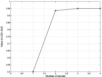
Fig. 3. Evolution of LOO-AUC versus the classifier size for the synthetic data set using the proposed algorithm.
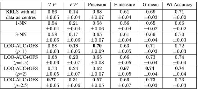
TABLE II
GENERALIZATIONPERFORMANCE OFCLASSIFICATION FORSYNTHETICDATASET
distribution was also generated, providing 1000 data samples for the majority class and 100 data samples for the minority class.
By using the estimation data set, the Gaussian kernel function is used as basis functions, where is set as 1. All estimation data examples were used to form the candidate center set . The regularization parameter was set as 1 10 . Taking 10 for illustration, the proposed maximal LOO-AUC-based forward selection algorithm (LOO - AUC OFS) was applied. The modeling process is illustrated in Fig. 3, in which it is seen that LOO-AUC increases over the forward regression step up to model size 3.
To illustrate the effect of the proposed algorithm of achieving a more balanced classification results for both classes, the full set of 110 kernels was used to construct a kernel classifier with regularized least squares parameter estimator (KRLS). The reg-ularization parameter 1 10 was applied. Other algorithms used for comparison are the -nearest neighbor classifiers (1-NN and 3-NN). For imbalanced data sets, there are several performance metrics widely used for comparison. All of them are based on values in the confusion matrix of Table I. The performance on TP and FP can be used to generate a single performance metric as geometric mean (G-mean), defined by
G-mean TP FP (33)
The G-mean value is a metric which favors balanced classifi-cation performance for two classes. In addition to TP, FP, and G-mean, there are precision [41] and F-measure [41] as defined by
Precision (34)
and
F-measure Precision TP
Fig. 4. Synthetic test data set and the decision boundary of (a) the regularized least squares 110-center kernel classifier with equal data weighting and (b) the derived three-term kernel classifier by the proposed algorithm.
TABLE III
EIGHTFOLDCROSS-VALIDATIONCLASSIFICATIONPERFORMANCE FORPIMAINDIANDIABETESDATASET
that it is impractical for KRLS to be applied to very large data samples. In addition, both KRLS and -nearest neighbor classi-fier will certainly be more computational expensive when eval-uating new data samples as they all involve calculation through the full estimation data set.
Example 2: The Pima Indians diabetes data set obtained from the University of California at Irvine (UCI) repository [42] contains 768 samples from two classes with 500 nega-tive samples and 268 posinega-tive samples. The posinega-tive class is interpreted as “tested positive for diabetes.” There are eight input features for the data samples. Initially, all eight input features are normalized to the range using the
opera-tion: , ,
, for . Then, the Gaussian kernel function is used as the basis func-tions, where is set as 1. As shown in Fig. 5, initially taking 2 and based on the whole data set, the model construction process using LOO-AUC model term selection is demonstrated by automatically deriving a kernel classifier with nine centers. The regularization parameter 1 10 was applied.
Then, the eightfold cross validation was used to investigate the effectiveness of the proposed algorithm. The proposed
al-gorithm with various values of were experimented with regu-larization parameter as 1 10 , in comparison with al-ternative approaches. The results of -nearest neighbor (1-NN and 3-NN) and a kernel classifier were used for comparison; the latter is based on the regularized least squares algorithm using all estimation data as centers and the regularization parameter of 1 10 . The results of the eightfold cross validation are shown in Table III. For models derived using equal weighting for data samples, the models have a low TP, i.e., weak detection capability for diabetes. The variation in performance in terms of TP and FP with respect to that of parameter is examined. is increased from 1 to 2.5 at a step of 0.5; it increased the detection capability at the cost of an increased FP. Based on G-mean and F-measures, it can be concluded that the choice of around two produced better models.
The models derived using the LOO - AUC OFS algorithm in eightfold cross-validation experiments have model sizes in the range of 4–24 centers.
Fig. 5. Evolution of LOO-AUC versus the classifier size for Pima Indians diabetes data set using the proposed algorithm.
TABLE IV
TWOFOLDCROSS-VALIDATIONCLASSIFICATIONPERFORMANCE FORHABERMANDATASET
and 81 positive samples. The positive class represents “the pa-tients who died within five years.” There are three input features for the data samples. The data set was randomly split into 50/50 for the twofold cross-validation experiments. Initially, all three input features are normalized to the range using the
oper-ation: , ,
, for . Then, the Gaussian kernel function is used as a basis func-tion, where is set as 1. The proposed algorithm with various values of was experimented with regularization parameter as 1 10 , in comparison with the -nearest neighbor (1-NN and 3-NN) and a kernel classifier that are based on the regularized least squares algorithm using all estimation data as centers and the regularization parameter of 1 10 . The re-sults of the twofold cross validation are shown in Table IV. For models derived using equal weighting for data samples, the models have a low TP, i.e., weak detection capability for the positive class. Experiments on the proposed algorithm were car-ried out by increasing from 1 to 4 at a step of 1. It is clear that
TP is increased at the cost of an increased FP. Based on the G-mean and F-measures, it can be concluded that the choice of
around three produced better models.
Example 4:The austempered ductile iron (ADI) material data set for automotive camshaft application [43] is used to study why fatigue cracks are initiated from the graphite nodules within the microstructure. There are nine features and two class labels (“crack” and “no crack”). The data set is very imbalanced with a total of 2923 samples in which 116 samples are “crack class,” and 2807 samples are “no crack class.” A cost-sensitive support vector machine (CS-SVM) and a cost-sensitive SUPANOVA model [43] were applied to investigate the data set [43]. The cost-sensitive SUPANOVA model used one-norm regularization to derive a reduced model set trading model interpretability with classification performance. They used a reduced training data set of 90 “crack” and 700 “no crack” data samples.
[image:10.594.134.455.374.518.2]TABLE V
GENERALIZATIONPERFORMANCE OFCLASSIFICATION FORADI DATASET
pairs of training/testing data set in order to make a com-parison with results of [43]. Initially, all nine input fea-tures are normalized to the range using the operation:
, ,
, for . Then, the Gaussian kernel function is used as a basis func-tion, where is set as 1. For each pair of training/testing data set, all the data samples in the training data set were used to form the candidate center set . The regularization parameter was set as 1 10 . The proposed maximal LOO-AUC-based forward selection algorithm LOO - AUC OFS was applied while was varied from 1 to 20. The classification results of the eight trials were listed in Table V. The results are quoted from [43] for comparison. The CS-SVM approach in [43] used a control sensitivity loss function [28] including weights for slacking variables of two classes, respectively. Lee [43] used a grid search by varying in the range [0.01, 10 000], and the best model in terms of best G-mean was found the model with ( 1, 0.1). To provide the overall performance on other criteria on precision, F-measure, G-mean, and weighted accuracy for SVM, CS-SVM, and SUPANOVA, these values are added based on Table I, (1), (2), and (33)–(35). It can be concluded that the choice of around 10–12 produced better models with competitive performance with the best CS-SVM ( 1, 0.1). For 12, the model size is between 3–7.
Example 5: The Satimage data set from the UCI repository [42] obtained from [44] contains 36 attributes that are numer-ical values for nine neighborhood pixels in four frequencies, and six class labels [44] denoting types of soil (or crop) of the cen-tered pixel. There are 9.73% samples of the data set from class 4 (damp grey soil) as the least prevalent class, and this was chosen to be classification target in this study . Data with other class labels were combined as a major class “not class 4,” con-taining 90.27% samples of the data set . The total number of data samples is 6435. The data set was split into ten pairs of training/test data sets using tenfold cross validation. The size of each training data set is, therefore, 5791. For each training
data set in turn, the experiments were repeated to obtain results for in the range of between 1–10.
Initially, all 36 input features are normalized to the range using the operation:
, , , for . Then, the Gaussian
kernel function is used
as a basis function, where is set as 1. In order to reduce the computational cost, 20% randomly drawn training data samples ( 1158) rather than all the training data samples were used to form the candidate center set . The regularization parameter was set very small as 1 10 since the training data set size is large. The proposed maximal LOO-AUC-based forward selection algorithm LOO - AUC OFS was repeat-edly applied to each training data set with different . The derived model size are between 15–30. In Table VI, the tenfold cross-validation results of the proposed approach were listed together with some other imbalanced data classifiers quoted from [35] for reference. It is worth mentioning that the RF approach used in [35] is a sophisticated classification tree approach with unparallel classification accuracy [5]. Note that the model derived from LOO - AUC OFS algorithm with a proper tends to achieve high performance over minority class trading off performance in the majority class. We do not claim the superiority over other imbalanced data modeling methods, as the best tradeoff between TP and FP is dependent upon the application. The purpose of the paper is to investigate the applicability of the algorithm for imbalanced data, especially in its capability to achieve a good balanced performance through the objective function (5). Note that it is easy to modify the algorithm by using other model selective criteria, e.g., F-mea-sure (35) in order to derive models with better performance for the specific measure of interest. The example indicates that the proposed algorithm can achieve good classifiers with simple model structure.
V. CONCLUSION
TABLE VI
TENFOLDCLASSIFICATIONPERFORMANCE FORSATIMAGEDATASET
misclassification rate over all data samples. In real applications, imbalanced data sets are common where the objective is to achieve a high accuracy for minority class as well as that of majority class. Conventional classifiers tend to produce unfavorable classification results for minority class unless the issues caused by the imbalance between classes are addressed in an appropriate manner. A new two-class kernel classifier construction algorithm uses OFS in order to optimize the model generalization for imbalanced data sets. The new kernel classifier identification algorithm is based on a new ROWLS and the model selective criterion of a maximal LOO-AUC of the ROCs. The new regularized orthogonal weighted least squares algorithm as parameter estimator is developed in the framework of forward orthogonal selection. Based on the orthogonalization procedure, the computing of LOO-AUC is performed using analytic formula rather than actually splitting the estimation data set. Consequently, the proposed algorithm can achieve minimal computational expense via a set of for-ward recursive updating formula in the search of terms with maximal LOO-AUC value. Several examples have been pro-vided to demonstrate the proposed algorithm is a viable, highly computational, and efficient alternative approach for building two-class classifier for imbalanced data sets.
APPENDIX
LOO MODELINGRESIDUALS OFREGULARIZEDOWLS
Following (18), the regularized parameter vector estimator based on orthogonal weighted least squares algorithm is
(36)
where is a unit matrix. Substitute (36) into (19) of the model residual representation to yield
(37)
If the data sample indexed at is deleted from estimation data set, the regularized LOO model parameter vector based on OWLS is given by
(38) where denotes the weighted output vector , with its th element as . and denote the LOO regres-sion matrix and weighted output vector, respectively. By deriva-tion, it can be shown that
(39)
(40) The LOO modeling errors evaluated at , based on the regular-ized orthogonal weighted least squares, are given by
(41)
Equation (39) and using the matrix inversion lemma yields
(42) and
(43)
Substituting (40) and (43) into (41) yields
Applying (37) to (44) yields
(45)
ACKNOWLEDGMENT
The authors would like to thank Dr. P. A. S. Reed and Dr. K. K. Lee for providing the austempered ductile iron (ADI) data set and the reviewers for their valuable comments.
REFERENCES
[1] M. Stone, “Cross validatory choice and assessment of statistical pre-dictions,”J. Roy. Stat. Soc., Ser. B, vol. 36, pp. 117–147, 1974. [2] R. O. Duda, P. E. Hart, and D. G. Stork, Pattern Classification. New
York: Wiley, 2001.
[3] L. Breiman, “Bagging predictors,”Mach. Learn., vol. 24, no. 2, pp. 123–140, 1996.
[4] ——, “Arcing classifiers,”Ann. Stat., vol. 26, no. 3, pp. 801–849, 1996. [5] ——, “Random forests,”Mach. Learn., vol. 45, no. 1, pp. 5–12, 2001. [6] R. A. Jacobs, M. I. Jordan, S. J. Nowlan, and G. E. Hint, “Adaptive mixtures of local experts,”Neural Comput., vol. 3, pp. 79–87, 1991. [7] C. Ji and S. Ma, “Combinations of weak classifiers,” IEEE Trans.
Neural Netw., vol. 8, no. 1, pp. 32–42, Jan. 1997.
[8] E. M. Kleinberg, “Stochastic discrimination,”Ann. Math. Artif. Intell., vol. 1, no. 1–4, pp. 207–239, 1990.
[9] F. Provost and T. Fawcett, “Robust classification for imprecise envi-ronments,”Mach. Learn., vol. 42, pp. 203–231, 2001.
[10] R. Xu and D. Wunsch, II, “Survey of clustering algorithms,”IEEE Trans. Neural Netw., vol. 16, no. 3, pp. 645–678, May 2005. [11] V. Vapnik, The Nature of Statistical Learning Theory. New York:
Springer-Verlag, 1995.
[12] M. E. Tipping, “Sparse Bayesian learning and the relevance vector ma-chine,”J. Mach. Learn. Res., vol. 1, pp. 211–244, 2001.
[13] B. Scholkopf and A. J. Smola, Learning With Kernels: Support Vector Machine, Regularization, Optimization and Beyond. Cambridge, MA: MIT Press, 2002.
[14] X. Hong and C. J. Harris, “Nonlinear model structure design and construction using orthogonal least squares and D-optimality design,”
IEEE Trans. Neural Netw., vol. 13, no. 5, pp. 1245–1250, Sep. 2001. [15] S. Chen, S. A. Billings, and W. Luo, “Orthogonal least squares
methods and their applications to non-linear system identification,”
Int. J. Contr., vol. 50, pp. 1873–1896, 1989.
[16] S. Chen, Y. Wu, and B. L. Luk, “Combined genetic algorithm opti-mization and regularized orthogonal least squares learning for radial basis function networks,”IEEE Trans. Neural Netw., vol. 10, no. 5, pp. 1239–1243, Sep. 1999.
[17] S. Chen, X. Hong, and C. J. Harris, “Sparse kernel regression model-ling using combined locally regularized orthogonal least squares and D-optimality experimental design,”IEEE Trans. Autom. Control, vol. 48, no. 6, pp. 1029–1036, Jun. 2003.
[18] X. Hong, P. M. Sharkey, and K. Warwick, “A robust nonlinear identi-fication algorithm using press statistic and forward regression,”IEEE Trans. Neural Netw., vol. 14, no. 2, pp. 454–458, Mar. 2003. [19] S. Chen, X. Hong, C. J. Harris, and P. M. Sharkey, “Sparse modeling
using orthogonal forward regression with press statistic and regulariza-tion,”IEEE Trans. Syst., Man, Cybern., B: Cybern., vol. 34, no. 2, pp. 898–911, Apr. 2004.
[20] K. Z. Mao, “RBF neural network center selection based on fisher ratio class separability measure,”IEEE Trans. Neural Netw., vol. 13, no. 5, pp. 1211–1217, Sep. 2002.
[21] S. Chen, X. X. Wang, X. Hong, and C. J. Harris, “Kernel classifier con-struction using orthogonal forward selection and boosting with Fisher ratio class separability,”IEEE Trans. Neural Netw., 2006, to be pub-lished.
[22] K. Z. Mao and G. B. Huang, “Neuron selection for RBF neural network classifier based on data structure preserving criterion,”IEEE Trans. Neural Netw., vol. 16, no. 6, pp. 1531–1540, Nov. 2005.
[23] X. Hong, S. Chen, and C. J. Harris, “Fast kernel classifier construc-tion algorithm using orthogonal forward selecconstruc-tion to minimize leave-one-out misclassification rate,” inProc. 2nd Int. Conf. Intell. Comp. Pt. I, D. S. Huang, K. Li, and G. W. Irwin, Eds., Kuming, China, 2006, pp. 106–114.
[24] F. Provost, T. Fawcett, and R. Kohavi, “The case against accuracy es-timation for comparing induction algorithms,” inProc. 15th Int. Conf. Mach. Learn. (ICML), San Francisco, CA, 1998, pp. 443–453. [25] J. Leskovec and J. Shawe-Taylor, “Linear programming boost for
un-even datasets,” inProc. Int. Conf. Mach. Learn. (ICML), Washington, DC, 2003, pp. 456–463.
[26] G. Karakoulas and J. Shawe-Taylor, “Optimizing classifiers for imbal-anced training sets,” inProc. Neural Inf. Process. Workshop (NIPS’98), Denver, CO, 1998, pp. 253–259.
[27] P. D. Turney, “Cost-sensitive classification: Empirical evaluation of a hybrid genetic decision tree induction algorithm,”J. Artif. Intell. Res., no. 2, pp. 369–409, 1995.
[28] K. Veropoulos, C. Campbell, and N. Cristianini, “Controlling the sensi-tivity of support vector machine,” inProc. Int. Joint Conf. Artif. Intell. (IJCAI99), Stockholm, Sweden, 1999, vol. Workshop ML3, pp. 55–60. [29] G. Wu and E. Y. Chang, “Aligning boundary in kernel space for learning imbalanced dataset,” in Proc. 4th IEEE Int. Conf. Data Mining (ICDM 2004), Brighton, U.K., 2004, pp. 265–272.
[30] G. M. Fung and O. L. Mangasarian, “Multicategory proximal support vector machine classifier,”Mach. Learn., vol. 59, no. 1–2, pp. 77–97, 2005.
[31] N. Japkowicz, “Supervised versus unsupervised binary-learning by feedforward neural networks,”Mach. Learn., vol. 42, no. 1–2, pp. 97–122, 2001.
[32] S. Tan, “Neighbor-weighted k-nearest neighbor for unbalanced text corpus,”Expert Syst. Appl., vol. 28, pp. 667–671, 2005.
[33] M. Kubat, R. Holte, and S. Matwin, “Learning when negative examples abound,” inProc. Eur. Conf. Mach. Learn. (ECML 97), Prague, Czech Republic, 1997, pp. 1467–153.
[34] N. V. Chawla, K. W. Bowyer, L. O. Hall, and W. P. Kegelmeyer, “Smote: Synthetic minority oversampling technique,”J. Artif. Intell. Res., vol. 16, pp. 321–357, 2002.
[35] C. Chen, A. Liaw, and L. Breiman, “Using random forest to learn im-balanced data” Dept. Statistics, Univ. California Berkeley, Tech. Rep. 666, 2004.
[36] J. P. Egan, Signal Detection Theory and ROC Analysis. New York: Academic, 1975.
[37] J. A. Swets, Signal Detection Theory and ROC Analysis in Psychology and Diagnostics: Collected Papers. Mahwah, NJ: Lawrence Erlbaum Associates, 1996.
[38] R. H. Myers, Classical and Modern Regression With Applications, 2nd ed. Boston, MA: PWS-Kent, 1990.
[39] D. J. Mackay, “Bayesian interpolation,”Neural Comput., vol. 4, no. 3, pp. 415–447, 1992.
[40] D. W. Marquardt, “Generalised inverse, ridge regression, biased linear estimation and nonlinear estimation,”Technometrics, vol. 12, no. 3, pp. 591–612, 1970.
[41] C. van Rijsbergen, Information Retrieval. London, U.K.: Butter-worths, 1979.
[42] S. Hettich, C. L. Blake, and C. J. Merz, Repository of Machine Learning Databases Univ. California Irvine, 1998 [Online]. Available: http://www.ics.uci.edu/~mlearn/MLRepository.html
[43] K. K. Lee, C. J. Harris, S. R. Gunn, and P. A. S. Reed, “Classification of imbalanced data with transparent kernel,” inProc. INNS/IEEE Int. Joint Conf. Neural Netw. (IJCNN), Washington, DC, 2001, pp. 2410–2415. [44] UCL Machine Learning Group, Elena Database 2004 [Online].
Avail-able: http://www.dice.ucl.ac.be/mlg/?page=elena
Xia Hong(SM’02) received the B.Sc. and M.Sc. de-grees from the National University of Defense Tech-nology, Hunan, P.R. China, in 1984 and 1987, respec-tively, and the Ph.D. degree from the University of Sheffield, Sheffield, U.K., in 1998, all in automatic control.
intelligent control, neural networks, pattern recognition, learning theory, and their applications. She has published over 60 research papers, and coauthored a research book.
Dr. Hong was awarded a Donald Julius Groen Prize by Institution of Mechan-ical Engineers (IMechE) in 1999.
Sheng Chen(SM’97) received the B.Eng. degree in control engineering from the East China Petroleum Institute, Shandong, China, in 1982, the Ph.D. degree in control engineering from the City University at London, London, U.K., in 1986, and the D.Sc. degree from the University of Southampton, Southampton, U.K., in 2005.
He joined the University of Southampton, Southampton, U.K., in September 1999. He pre-viously held research and academic appointments at the Universities of Sheffield, Edingburgh, and Portsmouth, U.K. He has published over 200 research papers. His recent research work includes adaptive nonlinear signal processing, modeling and identification of nonlinear systems, neural network research, finite-precision digital controller design, evolutionary computation methods, and optimization.
Chris J. Harrisreceived the B.Sc. degree from the University of Leicester, Leicester, U.K., in 1967, the M.A. degree from Oxford University, Oxford, U.K., in 1976, and the Ph.D. degree from the University of Southampton, Southampton, U.K., in 2002, all in electrical engineering.
He is now with the University of Southampton, Southampton, U.K. He previously held appointments at the Universities of Hull, UMIST, Oxford, and Cranfield, and he was employed by the U.K. Ministry of Defence. He has authored or coauthored 12 books and over 400 research papers. His research interests are in the area of intelligent and adaptive systems theory and its application to intelligent autonomous systems, management infrastructures, intelligent control and estimation of dynamic processes, multisensor data fusion, and systems integration.