Shape optimization of conductive-media interfaces using an IGA-BEM solver

Shape Optimization of conductive-media interfaces that maximize

heat transfer using a BEM-Isogeometric solver

K.V. Kostasa,∗, M.M. Fyrillasb, C.G. Politisc, A.I. Ginnisd, P.D. Kaklisd,e a_{Department of Mechanical Engineering, Nazarbayev University, Kazakhstan}

b_{Department of Mechanical Engineering, Frederick University, Cyprus}

c_{Department of Naval Architecture, Technological Educational Institute of Athens, Greece} d_{School of Naval Architecture & Marine Engineering, National Technical University of Athens, Greece}

e_{Department of Naval Architecture, Ocean and Marine Engineering, University of Strathclyde, UK}

Abstract

In this paper, we present a method that combines the Boundary Element Method (BEM) with IsoGeometric Analysis (IGA) for numerically solving the system of Boundary Integral Equations (BIE) arising in the context of a 2-D steady-state heat conduction problem across a periodic interface separating two conducting and conforming media. Our approach leads to a fast converg-ing solver that achieves the same level of accuracy for fewer degrees of freedom, when compared with low-order BEM. Additionally, an optimization procedure is developed and test cases of in-terface’s shape optimization, with the aim of heat transfer maximization under given constraints, are demonstrated.

Keywords: Isogeometric Analysis, NURBS, Heat Transfer, Shape optimization

1. Introduction

Consider a 2-dimensional slab of thicknessH, with flat and isothermal upper and lower surfaces at temperature T1 and T2, respectively. The heat flux is q00 =k(T2−T1)/H [1], where k is the

thermal conductivity. Any extension from the surfaces of the slab would result in a reduction of the heat flux and any depression would result in an enhancement of the heat flux based on the inclusion theorems [2] and physical intuition. If the surfaces are not flat, but rather they are wavy and periodic with zero mean, the heat flux is enhanced depending on the geometry of the surface. For small amplitude corrugations, the enhancement of the heat flux is proportional to the square of the amplitude of the corrugations [3]. An isoperimetric optimization algorithm developed by Leontiou, Fyrillas & Kotsonis [4] has revealed that there is an optimum periodic geometry that maximizes the heat flux. Furthermore, if one of the surfaces of the slab is subjected to convection, then a single parameter optimization revealed the existence of a critical Biot number [5, 6] associated with extended surfaces, and the existence of a critical depth and thickness associated with embedded isothermal pipes [7, 8].

Next, consider a flat interface separating two slabs with thicknesses H1 andH2 and

conduc-tivities k1 and k2, respectively. If the exposed surfaces are flat and isothermal with

temper-ature T1 and T2, the heat flux can be obtained using the concept of thermal resistance to be q00= (T2−T1)/(H1/k1+H2/k2). Any extension of the interface from the high conductivity

mate-rial into the low conductivity matemate-rial would result in an enhancement of the heat flux, while any depression would result in its reduction. For a wavy, periodic interface with zero mean, the results are similar to those of a single slab; there is an enhancement of the heat flux, which depends on the geometry of the interface, and for small amplitude corrugations the enhancement is proportional to the square of the amplitude of the corrugations [3]. An isoperimetric optimization algorithm developed by Fyrillas, Leontiou, & Kostas [9] revealed that there is an optimum periodic geometry that maximizes the heat flux.

In the above references [4, 9], besides optimum corrugations, the authors also consider the optimal design of high conductivity inserts, and the optimal design of fins. The optimization problems considered are shape optimization problems and fall into the general area of inverse problems. In general, inverse problems associated with heat transfer have as a constraint the conduction or the conduction-convection partial differential equation. The objective function, any additional constraints and the variables of the optimization vary, depending on the application. For example, the objective function can be the difference between the computed temperature and the measured/prescribed temperature and the unknowns can be the boundary conditions, physical properties or the geometry of the configuration [10, 11, 12, 13, 14, 15]. Another example is to have the heat flux as the objective function and obtain the shapes that optimize it [16, 17, 18, 19, 20, 21, 9].

In general, inverse problems are ill-posed due to random errors in the numerical solution of the governing partial differential equation, and due to the sensitivity of the objective function on the constraint and the parameters; for example a small change in the parameters could lead to an enormous change in the estimated model, and/or there could be an infinite number of ge-ometries with approximately the same heat flux. Hence the solver gets trapped in local minima or diverges. Regarding inverse shape optimization problems, remedies to address the ill-possing include mapping the physical domain onto a fixed computational domain [16, 17, 18, 19, 20, 21] and redistribution of ill-ordered nodal points [12, 13, 14, 15], Tikhonov regularization [22], homog-enization [23], or transforming the problem into a parameter estimation by expanding the shape in terms of a small number of parameters, e.g. adaptive mesh [24], eigenfunction expansion [10], and mesh-morphing [25]. Recently, a method that proved effective is to use the boundary element method and define the variables of the optimization as the angles between adjacent elements [9].

direct heat transfer problems where only a single solution of the PDE is necessary [26, 27, 28], in inverse problems each iteration requires the solution of the PDE at least as many times as the number of the optimization variables. In addition, accuracy is very significant due to the sensitivity of the solution on the parameters of the optimization. Hence, where applicable, the boundary element method [29, 30, 31] provides a natural selection for the numerical solution of the PDE due to its superiority of handling, with high accuracy, a large number of elements and intricate wall geometries [16, 17, 18, 4, 19, 20, 21, 9].

In this work we reconsider the case of an interface separating two slabs, which was mentioned, above but this time we employ the isogeometric approach in its solution. The IsoGeometric Anal-ysis concept, introduced by Hughes et al (2005) [32] in the context of Finite Element Method, was extended to the Boundary Element Method by various authors, see, e.g., Politis et al (2009) [33], Simpson et al (2012) [34], Scott et al (2013) [35], Belibassakis et al (2013) [36], Peake et al (2013) [37], Simpson et al (2014) [38], Ginnis et al (2014) [39]. The developed Isogeometric-BEM is based on a NURBS representation of the interface curve and employs the very same basis of the geometry for representing the temperature (T) and its normal derivative (∂T

∂n) on the interface.

The Boundary Integral Equation is numerically solved by collocating at the Greville abscissas of the knot vector of the interface’s parametric representation. Numerical error analysis of the Isogeometric-BEM, using h-refinement technique (knot insertion), is performed and compared with classical low-order panel methods. Finally, the developed isogeometric-BEM is also demonstrated in the context of shape optimization with aim of acquiring the interface’s shape the maximizes heat transfer under given constraints.

2. Problem formulation

2.1. Continuous formulation

We consider a 2-D steady-state heat conduction problem across a periodic interface separating two conducting and conforming materials. The interface S is an L-periodic planar, continuous, free-form curve. At the outer boundaries of the two mediums we specify isothermal conditions, where, without loss of generality, we can assume ¯T1= 1 andT2= 0; see Fig. 1.

Having in mind to use the Boundary-Integral Equation method to solve the arising boundary-value problems, and in order to unify the use of Green’s function in both domains (materials), we transform the temperature field in medium 1 by setting T1 = ¯T1 −1, which results in a

homogeneous boundary condition on its outer boundary and a discontinuity of the temperature on the interface. Due to the periodicity of the interface we confine ourselves to a domain of length L and nondimensionalize lengths with the period L; see Fig. 2.

The temperature fields T1 andT2satisfy the following conditions:

L medium 2 conductivity κ2

medium 1 conductivity κ1

S

ΔΤ1=0

ΔΤ2=0

Τ1=1

Τ2=0

X Y

Figure 1: L-periodic interface between two conducting and conforming materials

S

X

Y

0

1

n

n

Sv,l

Sv,l

S

Sh

Ω

Ω

S

Sv,r

h

H

Figure 2: One period of the interface and domain boundaries

∆Ti(x, y) = 0, (x, y)∈Ωi, i= 1,2, (1)

where Ωi denotes the open domain occupied by materiali.

• Boundary conditions on the horizontal outer boundaries Si h:

Ti(x, y) = 0, (x, y)∈Shi, i= 1,2 (2)

• Periodic conditions on the vertical boundariesSi v:

Ti(0, y) =Ti(1, y), y∈[0, h1], i= 1,2 (3a) Ti,x(0, y) =Ti,x(1, y), y∈[h1, H], i= 1,2 (3b)

whereTi,xstands for the partial derivative ofTi with respect tox.

¯

T1(x, y) =T1(x, y) + 1 =T2(x, y), (x, y)∈S (4a) k1

∂T1(x, y) ∂n1

=−k2

∂T2(x, y) ∂n2

, (x, y)∈S, (4b)

whereni, i= 1,2 denote the normal vectors to the interface directed inwards to the domain Ωi.

In order to derive an integral-equation formulation of the above problem we introduce the periodic Green’s functions for the Laplace equation:

∆Gi(x,x0) =δ(x−x0), (x,x0)∈Ωi, i= 1,2, (5)

wherex= (x, y) andx0= (x0, y0), which satisfy the wall conditions (2) and the periodic conditions

(3a) and (3b). Using the method of images, these Green’s functions are given as follows (see [30]):

Gi(x,x0) =

1

4πln[cosh(2π(y−y0))−cos(2π(x−x0))]− − 1

4πln[cosh(2π(y−yi))−cos(2π(x−x0))]

(6)

wherey1=−y0,y2= 2H−y0andH is the dimensionless thickness of the composite wall.

As it can be easily seen from (6),Gi(x,x0), i= 1,2,have a logarithmic singularity asx→x0. By

applying Green’s second identity for the functions T1(x) and G1(x,x0),(x,x0)∈ Ω1, and using

equations (1-3b) we obtain the following Fredholm-type integral equation of the second kind for the temperature fieldT1(x),x∈S:

T1(x0)

2 =

Z

S

G1(x,x0) ∂T1(x) ∂n1(x)

d`(x)−

Z

S

T1(x)

∂G1(x,x0) ∂n1(x)

d`(x), x0∈S. (7)

Similarly, for the temperature fieldT2(x),x∈S we obtain, T2(x0)

2 =

Z

S

G2(x,x0) ∂T2(x) ∂n2(x)

d`(x)−

Z

S

T2(x)

∂G2(x,x0) ∂n2(x)

d`(x), x0∈S. (8)

Now, using relations (4a) and (4b), as well as the obvious relationn1(x) =−n2(x),x∈S, we can

write (8) as follows:

T1(x0) + 1

2 =−

Z

S

G2(x,x0) k1 k2

∂T1(x) ∂n1(x)

d`(x) +

Z

S

(T1(x) + 1)

∂G2(x,x0) ∂n1(x)

d`(x), x0∈S. (9)

Equations (7) and (9) are combined to give the final system of equations with respect toT1(x)

and∂T1(x)/∂n1(x),x∈S, which reads as follows: Z

S

G1(x,x0) ∂T1(x) ∂n1(x)

d`(x)−

Z

S

T1(x)∂G1(x,x0) ∂n1(x)

d`(x)−T1(x0)

2 = 0. (10a)

−k1

k2

Z

S

G2(x,x0) ∂T1(x) ∂n1(x)

d`(x) +

Z

S

T1(x)∂G2(x,x0) ∂n1(x)

d`(x)−T1(x0)

2 =

1

2−

Z

S

∂G2(x,x0) ∂n1(x)

d`(x). (10b)

Finally, the dimensionless heat transfer across the interface per period is defined by,

hT =

Z

S

∂T1(x) ∂n1(x)

2.2. A discrete IGA-BEM formulation

In this subsection we present a method that combines Boundary Element Method (BEM) with IsoGeometric Analysis (IGA) for solving numerically the system of boundary integral equations (10a) and (10b). IGA philosophy is equivalent to approximating the field quantities (dependent variables) of the boundary-value problem in question by the very same basis that is being used for representing (accurately) the geometry of the involved domain boundary. In our case the dependent variables are the temperature field and its normal derivative on the interfaceS,T1(x)

and ∂T1(x)

∂n1(x),x∈S, see Eqs. (10a) and (10b). For this purpose, we shall presume that the interface S can be accurately represented as a parametric NURBS curvex(t), t ∈[0,1], which is regular, i.e., the derivative vector is well defined and not vanishing. More specifically,

x(t) = (x(t), y(t)) :=

n

X

i=0

diRi,k(t), t∈I= [tk−1, tn+1] := [0,1], (12)

where {Ri,k(t)}in=0 is a rational B−spline basis of order k, defined over a knot sequence J = {t0, t1, . . . , tn+k}and possessing non-negative weightswi, i= 0, . . . , n, whilediare the associated

control points; see, e.g., Piegl & Tiller [40]. Using this parametric representation of the interface S, equations (10a) and (10b) can be written in the following form:

Z

I

G1(t, τ)∂T1(t) ∂n1(t)

kx(˙ t)kdt−

Z

I

T1(t)∂G1(t, τ) ∂n1(t)

kx(˙ t)kdt−T1(τ)

2 = 0. (13a)

−k1

k2

Z

I

G2(t, τ)∂T1(t) ∂n1(t)

kx(˙ t)kdt+

Z

I

T1(t)∂G2(t, τ) ∂n1(t)

kx(˙ t)kdt−T1(τ)

2 =

1

2−

Z

I

∂G2(t, τ) ∂n1(t)

kx(˙ t)kdt. (13b)

where, for the sake of simplicity, we defineT1(t) :=T1(x(t)) andG1(t, τ) :=G1(x(t),x(τ)).

In order to handle equations (13a) and (13b), in the context of IGA, we project, in a suitably defined manner, the temperature field T1(t) and its normal derivative _∂∂T_n1(t)

1(t) on the spline space Sk_(J(`)_),Sk_(J(0)_{) :=S}k_{(J), expressed in the form:}

T1,s(t) :=Ps(T1(t)) =

n+`

X

i=0 T1,iR

(`)

i,k(t), t∈I, R

(0)

i,k(t) :=Ri,k(t), (14)

h1,s(t) :=Ps

_∂T

1(t) ∂n1(t)

=

n+`

X

i=0 h1,iR

(`)

i,k(t), t∈I, R

(0)

i,k(t) :=Ri,k(t), (15)

where`∈<sub>N0</sub>denotes the number of knots inserted inI.Recalling the fundamental property of knot insertion, we can say that{Sk<sub>(J</sub>(`)_{), `∈}

N0} constitutes a sequence of nested finite

dimensional-spaces, i.e.,Sk_(J(`)<sub>)⊂ S</sub>k<sub>(J</sub>(`+1)_).

Introducing the projections (14) and (15) into equations (13a) and (13b) we obtain:

Z

I

G1(t, τ)

n+` X

i=0 h1,iR

(`)

i,k(t)kx(˙ t)kdt− Z

I n+` X

i=0 T1,iR

(`)

i,k(t)

∂G1(t, τ) ∂n1(t)

kx(˙ t)kdt−1 2

n+` X

i=0 T1,iR

(`)

i,k(τ) = 0. (16a)

−k1

k2

Z

I

G2(t, τ)

n+` X

i=0

h1,iR(_i,k`)(t)kx(˙ t)kdt+ Z

I n+` X

i=0

T1,iR_i,k(`)(t)

∂G2(t, τ) ∂n1(t)

kx(˙ t)kdt−1 2

n+` X

i=0

T1,iR(_i,k`)(τ) =

=1

2−

Z

I

∂G2(t, τ) ∂n1(t)

kx(˙ t)kdt. (16b)

Several methods are available for defining the projection Ps (see Eqs. (14) and (15)) onto the

finite-dimensional space Sk

(J(`)

) and discretizing equations (16a) and (16b), like Galerkin and collocation.

In the present work, a collocation scheme is adopted, which consists in projecting on Sk

(J(`)

) through

L 2

1

medium 1, κ = 1 medium 2, κ = 0.5

T=0 T=1

H

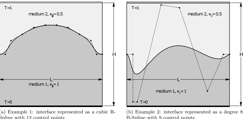
(a) Example 1: interface represented as a cubic B-Spline with 12 control points

1

2 medium 2, κ = 0.5

T=0

H

L T=1

medium 1, κ = 1

(b) Example 2: interface represented as a degree 8 B-Spline with 9 control points

Figure 3: Media Layout and interface shapes for examples 1 & 2.

abscissas associated with the knot vectorJ(`)_{. This leads to the following linear system for the unknown}

coefficientsT1,iandh1,i, i= 0, . . . , n+`:

n+`

X

i=0 h1,i

Z

I

G1(t, τj)R

(`)

i,k(t)kx˙(t)kdt

+

n+`

X

i=0 T1,i

Z

I

∂G1(t, τj)

∂n1(t)

R_i,k(`)(t)kx˙(t)kdt−1

2R

(`)

i,k(τj)

= 0,

(17a)

−k1 k2

n+`

X

i=0 h1,i

Z

I

G2(t, τj)R

(`)

i,k(t)kx˙(t)kdt

+

n+`

X

i=0 T1,i

Z

I

∂G2(t, τj)

∂n1(t)

R_i,k(`)(t)kx˙(t)kdt−1

2R

(`)

i,k(τj)

=1 2 −

Z

I

∂G2(t, τj)

∂n1(t)

kx˙(t)kdt. (17b)

The solution of the linear system defined by equations (17a) and (17b) provides the values ofT1,i

andh1,i, i= 0, . . . , n+`, which can be used to calculate the heat transfer across the interfaceS

per period:

hT = n+`

X

i=0 h1,i

Z

I

R(_i,k`)(t)kx˙(t)kdt

. (18)

3. Numerical results & optimization examples

3.1. Convergence results

x

0 0.1 0.2 0.3 0.4 0.5 0.6 0.7 0.8 0.9 1

T

0.35 0.4 0.45 0.5 0.55 0.6 0.65

COMSOL IGA (21 DoFs) IGA (48 DoFs)

(a) Temperature distribution

x

0 0.1 0.2 0.3 0.4 0.5 0.6 0.7 0.8 0.9 1

norm

al flux

0.3 0.4 0.5 0.6 0.7 0.8 0.9

COMSOL IGA (21 DoFs) IGA (48 DoFs)

(b) Normal flux distribution

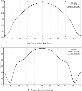
Figure 4: Comparison of temperature and normal flux distributions for the interface of example 1 against the corresponding COMSOL reference solutions.

The presented results are benchmarked against a reference solution from the commercial finite element computational package COMSOL[41], acquired with an extremely fine mesh of around 6×104 _{elements. Different numbers of degrees of freedom are utilized for calculating the values}

for the IGA-BEM approach and a low-order Boundary Element Method; see [9]. The resulting deviations from the reference solution, for both methods, are plotted on the same diagram so that the differences in the convergence rate and accuracy can be demonstrated. The agreement of IGA-BEM solution, both with respect to heat transfer values and the distributions of temperature & normal flux, is very satisfactory as will be demonstrated in the following discussion. We recall that the degrees of freedom (DoFs) for the IGA approach correspond to the number of the control coefficients used in the NURBS approximation of the temperatureT and normal fluxh; see Eqs. 14 and 15.

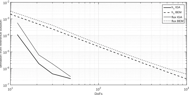
In Fig. 5, the deviation of heat transfer value (hT) from the COMSOL reference solution

along with theL2 norm of the normal flux distribution are depicted for the interface of Example

1; see Fig. 3a. The L2 norm for the normal flux distribution is computed as follows: L2 =

R1

0 |f(t(x))−fˆ(x)|

2_{dx, where ˆf(x) is the reference value of the normal flux at the longitudinal}

DoFs

101 102 103

deviation from reference solution

10-7 10-6 10-5 10-4 10-3 10-2

h_T IGA

h

T BEM

flux IGA flux BEM

Figure 5: Example 1 results: Deviation of BEM and IGA-BEM heat transfer (hT) and normal flux values from

COMSOL reference solution.

and the low-order BEM are plotted in the same figure for several different number of DoFs, where we can easily see that the convergence rate for the IGA-BEM approach is very fast (≈ O(n4₎₎

and we can attain, with just 50 DoFs the same level of accuracy that requires 103 DoFs for the low-order BEM.

The same picture is revealed when examining deviation values for hT and normal flux

distri-butions in the case of the 2nd example’s interface; see Fig. 3b. Specifically, as can be seen in Fig. 6, we once again get very fast convergence rates for the IGA-BEM approach and the accuracy attained with just 50 DoFs is even better than the one attained with 103_{DoFs with the low-order}

BEM approach. In this case the reference solution has been attained from COMSOL with an extremely fine mesh of 57945 elements.

3.2. Shape optimization

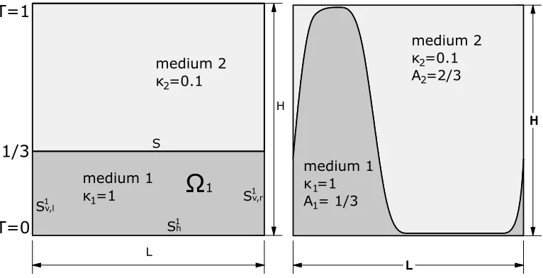
In the first optimization example, we assume that we start with two media of infinite length and equal thicknesses (H1 =H2 = 0.5H) with their contact surface (interface) being a straight

line as depicted in Fig. 7a. Obviously, within the periodL, each medium has an area of 0.5 square units and our optimization goal is to modify the two media’s distribution so that the heat transfer, between the two media, is maximized while the area for each one of them remains constant. Fur-thermore, we assume that the top surface of the bilayered construction is an isothermal boundary with a temperatureT = 1K, while the bottom surface is once again isothermal with a temperature equal to 0 degrees. Finally, we assume that the conductivity coefficient for the bottom medium (medium 1) isκ1= 1_mKW , while for the top medium (medium 2) isκ2= 0.1_mKW .

As discussed in previous sections, we may represent the interface between the two conductive media as a B-Spline curvec(t) = (cx(t), cy(t)) =Pn_i=0biNi,k(t), t∈[0,1], wherebi, i= 0, . . . , n

are the curve’s control points, k−1 is the curve’s degree and Ni,k are the kth order B-Spline

bases. In this example, we assume that it is represented as a cubic spline (k= 4) with 12 control points, i.e.,n+ 1 = 12. All control points have ay-coordinate equal to 0.5 (yi= 0.5, i= 0, . . . ,11)

while their x-coordinates have as follows x ={0 9,

1 18,

1 9,

2 9,

3 9,

4 9,

5 9,

6 9,

7 9,

8 9,

17 18,

9

9}. Assuming that

we keep thex-coordinates constant, then, with the aid of Eq. 15, we can state our heat transfer (hT) optimization problem as follows:

maxhT(y) = max

Z 1

0

h(t,y)kc˙(t,y)kdt= min 1 hT(y)

DoFs

101 102 103

deviation from reference solution

10-9 10-8 10-7 10-6 10-5 10-4 10-3 10-2

h_T IGA

h

T BEM

flux IGA flux BEM

Figure 6: Example 2 results: Deviation of BEM and IGA-BEM heat transfer (hT) and normal flux values from

COMSOL reference solution.

L

H

T=0

T=1

medium 1 κ =1₁

medium 2 κ =0.1₂

S

S1v,l

S1h

S1v,r

Ω

(a) Two media of infinite length with equal thicknesses in contact.

L

H

medium 1

κ

=1

A = 0.5

medium 2

κ

=0.1

A =0.5

(b) Optimum interface geometry under the straint of equal areas for the two media in con-tact.

DoFs

30 35 40 45 50 55 60 65 70 75

Deviation (L

2

)

10-10 10-9 10-8 10-7 10-6 10-5

10-4 hT

Temperature Flux

Figure 8: Deviation of optimum shape heat transfer (hT), temperature & normal flux distribution from COMSOL’s

solution, using approximately 5×104elements. Temperature and flux deviations are measured using theL2 norm

whilehT deviation is depicted as a percentage of COMSOL’s value.

subject to:

y11=y10=y1=y0 (20a)

I

∂Ω1

(cx(t,y) ˙cy(t,y)−cy(t,y) ˙cx(t,y))dt= 1, ∂Ω1=Sh1∪S

2

v,r∪S∪S

1

v,l (20b)

0.01≤yi≤0.99 (20c)

The first constraint (Eq. 20a) guarantees the periodicity and G1 continuity of our interface while the second constraint (Eq. 20b) enforces the area-equality for the two media. Obviously, in this particular case where the interface curve S is a function, Eq. 20b can be simplified as

R1

0 cy(t,y) ˙cx(t,y)dt= 0.5. Finally, due to Eq. 20a the design space drops from R 12 _to

R9 which

essentially means that the design vectory appearing in Eq. 19 isy={y0, y2, . . . , y9}and

equiva-lently the set of unknown control points isbi= (₉i, yi)T, i= 0,2,3, . . . ,9.

Several deterministic and guided random search algorithms have been tested which converged to a very similar shape with the best results, with respect tohT value, coming out of matlab’s

Genetic Algorithm implementation. The resulting optimum shape of the interface is depicted in Fig. 7b where a hT value of 0.4688 has been achieved. In comparison, the heat transfer for the

straight-line interface, is equal tohT0 = 1 0.5·κ1

κ₂+H−0.5

≈0.1818; see [9]. The resulting value of the heat transfer for the optimum interface along with the temperature and normal flux distribution along it have been verified with the commercial FEM computational package COMSOL as depicted in Fig. 8. As can be seen in Fig. 8 for the case of 30 DoFs, which were used during optimization, thehT value deviates only around 0.008% from the COMSOL acquired value. Finally, in Fig. 9,

the optimization history for the 1st shape optimization example is depicted, where Fig. 9a includes the complete optimization history while Fig. 9b is limited to results after the first 600 iterations. In the second optimization example, we once again assume that we start with two media of infinite length having as contact surface an infinite straight line as depicted in Fig. 10a. However, this time the two media have unequal thicknesses. Assuming once again a height ofH= 1 for the bi-layered structure, the two media will have an area of 1/3 and 2/3 square units within a period of L= 1 as is also depicted in Fig. 10a. The boundary conditions and conductivity coefficients are the same ones used in the first optimization example.

Iteration No

100 ₁₀1 ₁₀2 ₁₀3 ₁₀4 ₁₀5

1/h

T

2.5 3 3.5 4 4.5

5 _instances

optimum

(a) All iterations

Iteration No

103 ₁₀4

1/h

T

2.13 2.14 2.15 2.16 2.17 2.18 2.19 2.2

instances optimum

(b) Iterations 600 to end

L

H

T=0

T=1

medium 1 κ₁ =1

medium 2 κ =0.1₂

1/3

S1v,l

S1h

S1v,r

Ω

(a) Two media of infinite length and unequal thick-nesses in contact.

L

H

medium 1

κ =1

A = 1/31₁

medium 2 κ =0.1 A =2/322

(b) Optimum interface geometry subject to

con-stant medium-area constraint (A1=1₃, A2= 2₃)

Figure 10: Second optimization example

appropriately positioning the next to last control point. Hence, since x-coordinates are distributed uniformly1_{, the actual optimization problem variables are the y-coordinates of the control points}

excluding the first and the last two of them. Thus, assuming that we represent our interface with a cubic B-Spline consisting of 13 control points, we can state our heat transfer (hT) maximization

problem as follows:

maxhT(y) = max

Z 1

0

h(t,y)kc˙(t,y)kdt= min 1 hT(y)

(21)

subject to:

y12=y0=

1

3 (22a)

y1−y0 x1−x0

= y12−y11 x12−x11

(22b)

I

∂Ω1

(cx(t,y) ˙cy(t,y)−cy(t,y) ˙cx(t,y))dt=

2

3, ∂Ω1=S

1

h∪S

2

v,r∪S∪S

1

v,l (22c)

0.01≤yi≤0.99 (22d)

As in the first case, Eq.22c can be substituted by R1

0 cy(t,y) ˙cx(t,y)dt = 1

3, since the interface S is a functional curve. Furthermore and similar to the first optimization example, deterministic and evolutionary algorithms have been employed in the solving process. All algorithms converged practically in the same interface-shape shown in Fig. 10b while achieving a heat transfer equal to 0.3997. In comparison, the straight line interface achieves a heat transfer rate equal tohT0 =

1 2 3

κ1 κ₂+H−23

≈0.142857

4. Conclusions and future work

In the present work, an isogeometric boundary element method (IGA-BEM) is applied for solving the BIE system associated with the 2-D steady-state heat transfer problem across a periodic

1_{with the possible exception of the next to last control point that is positioned in a way that satisfiesG}1

interface separating two conducting and conforming media. The isogeometric concept, in this context, is based on the exploitation of the same NURBS basis, used for the exact representation of interface’s geometry, to approximate, via refinement, the physical quantities of temperature and normal heat flux.

The enhanced accuracy and efficiency of the present method has been demonstrated for two free-form interface geometries. The accuracy achieved for temperature & normal flux distributions with 21 and 48 DoFs is checked against the results acquired by the commercial computational package COMSOL with an extremely fine mesh of around 6×104 _{elements. Furthermore, the}

superior convergence rate of our IGA-BEM approach is compared with convergence rates achieved by classical low order BEM for the same two interface geometries.

Finally, a simple parametric model for the interface’s geometry is devised and employed in finding the optimum shape that maximizes heat transfer between the two media for two sets of varying geometrical constraints.

Future work is planned towards further exploitation of the developed approach in shape opti-mization and the extension of this work for additional heat transfer problem formulations.

References

[1] F. P. Incropera, D. P. DeWitt, Fundamentals of Heat and Mass Transfer, CRC Press, 2002.

[2] M. A. Lavrentev, B. V. Shabat, Methods of the theory of functions of complex variable, Nauka, Moscow, 1965, 1965.

[3] M. M. Fyrillas, C. Pozrikidis, Conductive heat transport across rough surfaces and interfaces between two conforming media, Int. J. Heat Mass Transfer 44 (2001) 1789–1801.

[4] T. Leontiou, M. Kotsonis, M. M. Fyrillas, Optimum isothermal surfaces that maximize heat transfer, Int. J. Heat Mass Transfer 63 (2013) 13–19.

[5] T. Leontiou, M. M. Fyrillas, Critical biot number of a periodic array of rectangular fins, ASME, J. Heat Transfer 138 (2016) 024504–1–024504–4.

[6] M. M. Fyrillas, S. Ospanov, U. Kaibaldiyeva, Critical biot numbers of periodic arrays of fins, ASME, Journal of Thermal Science and Engineering Applications 9 (2017) 044502–1–044502– 6.

[7] M. M. Fyrillas, H. A. Stone, Critical insulation thickness of a slab embedded with a periodic array of isothermal strips, Int. J. Heat Mass Transfer 54 (2011) 180–185.

[8] M. M. Fyrillas, Critical depth of buried isothermal circular pipes, Heat Transfer Engineering 39 (2018) 51–57.

[9] M. M. Fyrillas, T. Leontiou, K. V. Kostas, Optimum interfaces that maximize the heat transfer rate between two conforming conductive media, International Journal of Thermal Sciences 121 (2017) 381–389.

[10] H. Harbrecht, J. Tausch, On the numerical solution of a shape optimization problem for the heat equation, SIAM J. Scientific Computing 35 (2013) 104–121.

[11] M. J. Colaco, H. R. B. Orlande, G. S. Dulikravich, Inverse and optimization problems in heat transfer, J. of the Braz. Soc. of Mech. Sci. Eng. 28 (2006) 1–24.

[12] F. Mohebbi, M. Sellier, Three-dimensional optimal shape design in heat transfer based on body-fitted grid generation, Int. J. Comp. Methods Eng. Science and Mechanics 14 (2013) 473–490.

[14] C.-H. Cheng, C.-Y. Wu, An approach combining body-fitted grid generation and conjugate gradient methods for shape design in heat conduction problems, Num. Heat Transfer, Part B 37 (2000) 69–83.

[15] C.-H. Cheng, M.-H. Chang, Shape design for a cylinder with uniform temperature distribution on the outer surface by inverse heat transfer method, Int. J. Heat Mass Transfer 46 (2003) 101–111.

[16] M. M. Fyrillas, Shape optimization for 2d diffusive scalar transport, Optimization and Engi-neering 10 (2009) 477–483.

[17] M. M. Fyrillas, Heat conduction in a solid slab embedded with a pipe of general cross-section: shape factor and shape optimization, Int. J. Eng. Sci. 46 (2008) 907–916.

[18] M. M. Fyrillas, Shape factor and shape optimization for a periodic array of isothermal pipes, Int. J. Heat Mass Transfer 53 (2010) 982–989.

[19] T. Leontiou, M. M. Fyrillas, Shape optimization with isoperimetric constraints for isothermal pipes embedded in an insulated slab, ASME, J. Heat Transfer 136 (2014) 94502–1–094502–6.

[20] T. Leontiou, M. M. Fyrillas, Critical thickness of an optimum extended surface characterized by uniform heat transfer coefficient, arXiv:1503.05148 [physics.class-ph].

[21] T. Leontiou, M. Ikram, K. Beketayev, M. M. Fyrillas, Heat transfer enhancement of a periodic array of isothermal pipes, Int. J. Thermal Science 104 (2016) 480–488.

[22] A. N. Tikhonov, V. Y. Arsenin, Solution of Ill-Posed Problems, Winston & Sons, Washington, DC, 1977.

[23] g. Allaire, Shape Optimization by the Homogenization Method, Springer-Verlag, New York, 2002.

[24] P. Morin, R. Nochetto, M. S. Paulettim, M. Verani, Adaptive finite element method for shape optimization, ESAIM: COCV 18 (2012) 1122–1149.

[25] F. de Gournay, J. Fehrenbach, F. Plouraboue, Shape optimization for the generalized graetz problem, Struct. Multidisc. Optim. 49 (2014) 993–1008.

[26] M. M. Fyrillas, Advection-dispersion mass transport associated with a non-aqueous-phase liquid pool, J. of Fluid Mech. 413 (2000) 49–63.

[27] M. M. Fyrillas, K. E. J., Advection-dispersion mass transport associated with a non-aqueous-phase liquid pool, Trans. Porous Media 55 (2004) 91–102.

[28] M. Ioannou, M. M. Fyrillas, H. Doumanidis, Approximate solution to fredholm integral equa-tions using linear regression and applicaequa-tions to heat and mass transfer, Eng. Anal. Bound. Elem. 36 (2012) 1278–1283.

[29] C. A. Brebbia, Boundary Elements: An Introductory Course, Computational Mechanics; 2nd edition, 1992.

[30] C. Pozrikidis, A practical guide to boundary element methods with the software library BEMLIB, CRC Press, 2002.

[31] W.-T. Ang, A Beginner’s Course in Boundary Element Methods, Universal Publishers, 2007.

[33] C. Politis, A. Ginnis, P. Kaklis, K. Belibassakis, C. Feurer, An isogeometric BEM for exterior potential-flow problems in the plane, in: 2009 SIAM/ACM Joint Conference on Geometric and Physical Modeling, 2009.

[34] R. Simpson, S. Bordas, J. Trevelyan, T. Rabczuk, A two-dimensional Isogeometric Bound-ary Element Method for elastostatic analysis, Computer Methods in Applied Mechanics and Engineering 209–212 (2012) 87–100.

[35] M. A. Scott, R. N. Simpson, J. A. Evans, S. Lipton, S. P. A. Bordas, T. J. R. Hughes, T. Sederberg, Isogeometric boundary element analysis using unstructured T-splines, Computer Methods in Applied Mechanics and Engineering 254 (0) (2013) 197 – 221. doi:http://dx.doi.org/10.1016/j.cma.2012.11.001.

URLhttp://www.sciencedirect.com/science/article/pii/S0045782512003386

[36] K. A. Belibassakis, T. P. Gerosthathis, K. V. Kostas, C. G. Politis, P. D. Kaklis, A.-A. Ginnis, C. Feurer, A BEM-Isogeometric method for the ship wave-resistance problem, Ocean Engineering 60 (2013) 53–67.

[37] M. Peake, J. Trevelyan, G. Coates, Extended isogeometric boundary element method (XIBEM) for two-dimensional Helmholtz problems, Computer Methods in Applied Mechanics and Engineering 259 (2013) 93–102.

[38] R. N. Simpson, M. A. Scott, M. Taus, D. C. Thomas, H. Lian, Acoustic isogeometric boundary element analysis, Computer Methods in Applied Mechanics and Engineering 269 (2014) 265– 290.

[39] A. I. Ginnis, K. V. Kostas, C. G. Politis, P. D. Kaklis, K. A. Belibassakis, T. P. Gerostathis, M. A. Scott, T. J. R. Hughes, Isogeometric Boundary-Element Analysis for the Wave-Resistance Problem using T-splines, Computer Methods in Applied Mechanics and Engi-neering, submitted 2014.

[40] L. Piegl, W. Tiller, The Nurbs Book, 2nd Edition, Springer Verlag, 1997.