18th International Conference on Structural Mechanics in Reactor Technology (SMiRT 18) Beijing, China, August 7-12, 2005 SMiRT18-B01-4
A SIMPLE BOUNDARY ELEMENT FORMULATION FOR SHAPE
OPTIMIZATION OF 2D CONTINUOUS STRUCTURES
Luciano Mendes Bezerra*
University of Brasília – UnB
Department of Civil Engineering
70910-900 - Brasília, DF – Brazil
E-mail: [email protected]
Jarbas de Carvalho Santos Júnior
University of Brasília – UnB
Department of Civil Engineering
70910-900 - Brasília, DF – Brazil
E-mail: [email protected]
Arlindo Pires Lopes
University of Brasília – UnB
Department of Civil Engineering
70910-900 - Brasília, DF – Brazil
E-mail: [email protected]
André Luiz A. C. Souza
University of Brasília – UnB
Department of Civil Engineering
70910-900 - Brasília, DF – Brazil
E-mail: [email protected]
ABSTRACT
For the design of nuclear equipment like pressure vessels, steam generators, and pipelines, among others, it is very important to optimize the shape of the structural systems to withstand prescribed loads such as internal pressures and prescribed or limiting referential values such as stress or strain. In the literature, shape optimization of frame structural systems is commonly found but the same is not true for continuous structural systems. In this work, the Boundary Element Method (BEM) is applied to simple problems of shape optimization of 2D continuous structural systems. The proposed formulation is based on the BEM and on deterministic optimization methods of zero and first order such as Powell’s, Conjugate Gradient, and BFGS methods. Optimal characterization for the geometric configuration of 2D structure is obtained with the minimization of an objective function. Such function is written in terms of referential values (such as loads, stresses, strains or deformations) prescribed at few points inside or at the boundary of the structure. The use of the BEM for shape optimization of continuous structures is attractive compared to other methods that discretize the whole continuous. Several numerical examples of the application of the proposed formulation to simple engineering problems are presented.
Keywords: Shape Optimization, Boundary Element, Minimization Methods.
1. INTRODUCTION
Structural engineers are concerned with the design of structural members as ideal as possible in terms of cost, weight, aesthetic shape, compliance to limiting values in stress or strain and, above all, safety. The reduction of weight in such ideal structural members is fundamental today because of the shortage in material resources and the rise in the price of materials and possessing. In shipbuilding engineering, for instance, the reduction in structural weight results not only in cost savings but also in less fuel consumption for navigation. The same reasoning can also be applied to other types of vehicles, such as automobiles, and, moreover, rockets and airplanes (Ricketts and Zienkiewicz, 1984). In the nuclear industry, in design of nuclear equipment like pressure vessels, pipelines, supporting lugs of steam generators, and many other applications, it is very important to optimize the shape of the structural systems to withstand prescribed loads such as forces, moments, pressures or limit the magnitude of referential values such as stress or strain to copy with suggestion from nuclear standards.
methods. Other area under development due to the popularization of digital computers is the area of mathematical programming, among others. Under certain criteria, mathematical programming may optimize a set of variables so that the value of the objective function will be at a minimum. In structural engineering, such variable may represent dimensions, stresses, strains, or deformations of structural members. We may want to know the minimum dimensions or even the ideal shape of a structural member so that it can hold specific loads without achieving prescribed limit state, such as instability, yield stress, or large deformation, among others (Fox, 1973 and Gill; Murray; Wright, 1981).
Some application of structural shape optimization may be (Ricketts and Zienkiewicz, 1984): a) reduction of the amount of construction material, mainly the structural material, in general more expensive, as in concrete dams; b) reduction in the self-weight of structures, mainly in aerospace vehicles, automobile, and ships; c) appropriate choice of construction material, between aluminum, steel, concrete, wood, fiber of carbon, etc. since some of the physical properties of such materials (module of elasticity and strength) can be considered as design variables; d) the type and shape of connections, including the number and the arrangement of rivets, bolts or welds. These examples illustrate that the area of shape optimization of structural members is very wide and with potential for countless applications. Recently, the boundary element method - due to its “meshless” feature - is being successfully incorporate into algorithms for shape optimization of continuous structural members.
The goal of this work is to propose a numerical formulation, based on the BEM, for shape optimization of continuous 2D structures under in-plane loads.
2. THE PROBLEM OF SHAPE OPTIMIZATION
The objective of this work is to find ideal shapes of plane structural members. To find the ideal shape, a set of reference values may be pursued or, alternatively, some stress, strain, and displacement components or equivalent stress or strain values may be taken to a minimum. The function expressing these goals is called the objective function. The shape of a structural member can be defined by design variables (here named v) and, in this work the boundaries of the structural member are discretized by boundary elements. The design variables v
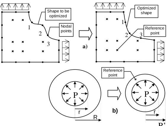
may be the coordinates (x and y) of boundary points or any other parameter (like radius, angles, etc.) that can define the geometry of the structural member. Fig.1 shows an example of a shape optimization of a pressure vessel support and a pipe cross-section. In the first case, the design variables are the coordinates x and y of the three nodal points (1, 2, 3) defining the part of the lug boundary to optimize. In the second case, the external radius R is the design variable to be optimized, while the internal radius “r” is kept constant for fluid flow reasons.
To find the optimal shape of the structures in Fig.1, a set of reference data
ϕ
ˆ
(in terms of quantities like stresses, strains, or displacements) may be given, or such quantities (or respective components) may be minimized at specific reference points. The goal is to look for a shape expressed by v so that reference data are matched or, alternatively, stresses, strains, or displacements are at a minimum. Note that such quantities are functions of the shape of the 2D structural member, therefore, function of the design variables v. Common ways to express these goals of minimization, in terms of v, is to write an objective functions F as shown in Eq.(1) and (2), respectively, for given reference data or for simple minimization of stresses, strains, or displacements. Other objective functions may easily be arranged.F
(
v
) =
∑∑
(
(
v
) -
or
F
(
v
) =
∑∑
(
v
)
= =m k
n j
kj
1 1 2
ϕ
2ˆ
kjϕ
)
= =
m k
n j
kj
1 1 2
ϕ
(1)F
(
v
) =
∑∑
= =m
k n
j kj
1 1
ϕ
(
v
) -
ϕ
ˆ
kjor
F
(
v
) =
∑∑
= =m
k n
j kj
1 1
ϕ
(
v
)
(2)
3 2 1
3 2 1 Shape to be
optimized
Nodal points
Optimized shape
Reference point
a)
P
R r
R
’
rP
b)
Reference point
Fig. 1: a) Design variables: x and y coordinates of nodal points 1, 2 e 3 b) Design variable is the external radius R
In the literature, there are many methods for the minimization of objective functions. In this work, the minimum of the objective function is pursued by the following three popular methods: Powell's, Conjugate Gradient, and BFGS Variable Metric Method (Fox, 1973 and Gill; Murray; Wright, 1981 and Press; Flannery; Teukolsky; Vetterling, 1986 and Reklaitis; Ravindran; Ragsdell, 1983 and Gallager; Zienkiewicz, 1973). They were chosen for this work because they are robust methods, their computer codes are easily available, and they are zero and first order methods which mean the second derivatives of the objective function with respect to the design variables are not necessary. These three methods are generally applied to the minimization of functions without any constraints on the design variables. The objective function in this work, however, has geometric constraints on the design variables. Such constraints are taken into consideration by heuristic approach to avoid unfeasible regions for the design variables during the minimization of the objective function.
3. REVIEW OF THE MINIMIZATION METHODS USED
As explained before, three methods are used in this paper for the minimization of the objective functions defined in Eqs. (1) or (2): Powell’s, Conjugate Gradient, and BFGS methods. In general, the methods differ in the way the minimum is achieved starting from an initial design variable vector vo. Consider the n-dimensional design variable vector v = {v1, v2, v3, ... vn}. For iteration “q+1”, a new value v is obtained according to
v
q+1=
v
q+
α
qS
q (3)where αq is a scalar, and Sq may be defined as the cyclic and unity coordinate vector specifying “n” search
direction such that S1 = {1, 0, 0, ... , 0}, S2 = {0, 1, 0, ... , 0}, and Sn = {0, 0, 0, ... , 1}. Initially, given an initial value for the design variable vo, a minimum for F(v) is obtained in each direction Sq (q = 1,…,n) according to appropriate scalar αq in Eq.(3). The minimum of F(v) may be achieved as a sequence of one-dimensional
minimization as a function of the scalar αq which represents a step length. If the number of design variables in v
is “n”, given an initial value vo, after “n” initial steps, vo becomes vn. Powell’s method defines the search direction (n+1) as
S
n+1=
v
n–
v
o (4)In the Conjugate Gradient method, the gradient of the function ∇F is required, so that the new search direction Sq+1 is calculated. Sq+1 is written as a linear combination of ∇F and the other searching directions S0, S1,
S2,..., Si obtained before, therefore
S
q+1=
−
∇
F
q+1+ β
S
q(5)
where: 2 2 1 q q
F
F
∇
∇
=
+β
and |∇Fq| is the norm of ∇Fq at iteration q. See, for instance, Eq.(7).In the BFGS Method, the objective function F(v) is expanded in Taylor's series around the point vq, and only three terms of this series are taken into account. The point vq represents the “qth” step approach to the minimum of F(v). In compact notation:
F
(
v
) =
F
(
v
q) +
∇
F
qT(
v
-
v
q) + 1/2 (
v
-
v
q)
TJ
q(
v
-
v
q)
(6)In the above expression, the term ∇FqT = [∇F(vq)]T is the gradient of the function F, and Jq is the Hessian
matrix, determined at vq . They are, respectively
∇
Fq
=
∂
∂
∂
∂
n q qv
v
F
v
v
F
)
(
)
(
1M
and
J
q=
( )
( )
( )
( )
∂
∂
∂
∂
∂
∂
∂
∂
∂
∂
2 2 1 2 1 2 2 1 2 n q n q n q qv
v
F
v
v
v
F
v
v
v
F
v
v
F
L
M
M
L
(7)Assuming
F
(v) is at a minimum, and, therefore, the gradient Eq.(6) is zero, then∇
F
T(
v
) =
∇
F
qT+
J
q(
v
-
v
q) =
0
(8)Notice that unless vq is at a minimum, ∇FqT≠0. Therefore, Eq.(8), may be rewritten for the “q+1” iteration as
J
qv
q-
J
qv
q+1= -
∇
F
qTor
v
q+1-
v
q=
v
q-1(
∇
F
qT)
(9)where the design variable v was substituted by vq+1 for the “q+1” approximation to the minimum. Eq.(9) may converge extremely fast in many problems, for instance, if the objective function is quadratic. The difficulties in using Eq.(9) are the calculation of the second derivative of F(v), the Hessian Jq, and the calculation of the
inverse of Jq. In the BFGS Method the inverse of the Hessian is approximated by the matrix Hq. This matrix
converges in each interaction to the exact Jq-1. Therefore, we have
v
q+1-
v
q=
H
q∇
F
qor
S
q=
H
q∇
F
q(10)
For obtaining the matrix Hq (Press; Flannery; Teukolsky; Vetterling, 1986), and Sq, BFGS uses the
following steps: a) The initial matrix H0 is assumed to be the identity matrix I. b) Compute the next matrix Hq at
each interactions “q” and c) Obtain vq+1 from Eq.(10) and verify for convergence
C
B
A
H
H
q=
q−1+
+
+
(11)Where
(
) (
)
(
)(
1)
(
)
[
]
[
(
)
]
(
1) (
1 1)
1 1 1 1 − − − − − − −
∇
−
∇
∇
−
∇
∇
−
∇
⊗
∇
−
∇
−
=
q q q q q q q q q q qF
F
F
F
F
F
F
F
H
H
H
B
(13)(
) (
)
[
H
]
u
u
C
=
∇
F
q−
∇
F
q−1 q−1∇
F
q−
∇
F
q−1⊗
(14)(
)
(
)(
)
(
(
1) (
1)
1)
1 1 1 1 1 − − − − − − − −
∇
−
∇
∇
−
∇
∇
−
∇
−
∇
−
∇
−
−
=
q q q q q q q q q q q q q qF
F
F
F
F
F
F
F
v
v
v
v
H
H
u
(15)In the expressions above, the symbol ⊗ represents the external product. With Sq determined, a new vq+1 in Eq.(3) towards the minimum can be obtained. BFGS and Conjugate Gradient are first order methods and need only the first derivatives of the objective function F. BFGS also needs the calculation of the Hessian matrix H
which is, approximately, calculated as explained before. In this work, the determination of the first derivative of the objective function is performed by finite difference as
i i i i i i i i
e
v
F
e
v
F
v
F
ξ
ξ
ξ
2
)
ˆ
(
)
ˆ
(
+
−
−
=
∂
∂
(16)where
e
ˆ
iis a unity vector in the direction of vi∈v, andξ
iis a small number.4. A BEM FORMULATION FOR SHAPE OPTIMIZATION
The boundary element method is a powerful numerical method and an alternative for engineering analysis - particularly where great precision in the results is required. The BEMcan be used in stress concentrationstudies, in problems with infinity or semi-infinity domains, in the solution of field equation (Laplace, Poisson, etc.), in problems of elasticity, and in fluid mechanics (Brebbia and Dominguez, 1989), among others. One important advantage of the BEM is that it, generally, requires only the discretization of the boundaries of the domain problem, instead of the whole continuous domain as in FEM or in FDM.
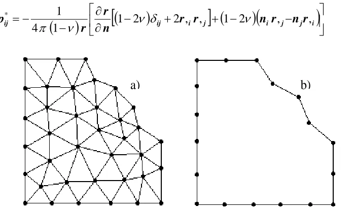
In the last decades, the FEM has been extensively used for structural optimization (Mota Soares; Rodrigues; Choi, 1984). In fact, the FEM presents great advantage for the optimization of particular structures such as trusses and frames, where the design variables may represent the length, the height, and the width dimensions of the member and its cross section. In continuous structures in 2D or 3D spaces, the use of FEM for structural optimization presents some disadvantages. The main disadvantage is the constant need to redefine the mesh every time the geometry of the structure changes. Remeshing tasks take great computational effort because each remesh generation involves redefinition of nodal points in terms of coordinate values, numbering, new element definitions, and corresponding new nodal connectivities. Fig.2 represents the mesh of a continuous 2D structure discretized with finite and boundary elements.
In this article, body forces will be regarded as small compared to other forces. Therefore, neglecting body forces, Somigliana’s Identity (Brebbia; Dominguez, 1989 and Banerjee; Butterfield, 1981) can be written as
∫
∫
ΓΓ
−
ΓΓ
=
u
p
d
p
u
d
u
li lk* k lk* k (17)Where Γ is the boundary of the structural member and represents the displacement component “l” located at a point “i”. As can be noticed in Eq.(17),
u
is expressed only in terms of boundary integrals. In such expression, the fundamental solutions for displacementu
and load are (Brebbia; Dominguez, 1989 and Banerjee; Butterfield, 1981) i lu
i l * lk * lkp
(
−
) (
−
)
+
=
ij i jij
r
r
r
G
u
3
4
ln
1
,
,
(
)
∂
[
(
−
)
+
]
+
(
−
)
(
−
)
∂
−
−
=
ij i j i j j iij
r
r
n
r
n
r
n
r
r
p
1
2
2
,
,
1
2
,
,
1
4
1
*ν
δ
ν
ν
π
(19)a)
b)
Fig. 2: a) Finite Element Mesh and b) Boundary Element Mesh
In Eq.(18) and (19),
δ
ij, r, and n are, respectively, the Kronecker delta, the distance between field and source points, and the normal to the boundary. The indices i and j refer to the Cartesian directions (x, y). ν and G are, respectively, Poisson’s coefficient, and the shear modulus. For more details see references (Brebbia; Dominguez, 1989 and Banerjee; Butterfield, 1981).The Somigliana’s Identity integral can be divided into smaller integrals each related to discrete boundaries defined as elements. In our case, the boundary elements are represented by three nodes and quadratic shape functions to interpolate the nodes. The shape functions (φ1, φ2, φ3), in terms of the non-dimensional parameter ξ,
are
(
1
2
1
1=
ξ
ξ
−
φ
)
,
φ
2(
1
−
ξ
2)
, and
(
1
)
2
1
3=
ξ
ξ
+
φ
(20)Partitioning the boundary Γ into N elements, Eq.(17) can be rewritten as
∑
=∫
∑ ∫
= Γ ∗ Γ ∗
Γ
Φ
=
Γ
Φ
+
N j N j j j i ip
d
u
u
d
p
u
c
j j 1 1 (21)Using the Jacobian |J|, dΓ can be expressed in terms of the natural coordinate dξ, as
D
Γ
=
|
J
|
d
ξ where
2 / 1 2 2 2 1
+
=
Γ
=
ξ
ξ
ξ
d
dx
d
dx
d
d
J
(22)xi are the coordinates (traditionally, x1 = x and x2 = y) defining the geometry of the boundary element as
functions of the shape functions and the nodal coordinates. Putting Eq.(22) into Eq.(21), we get
j N j j N j i i
p
d
J
u
u
d
J
p
u
c
j j∑ ∫
∑ ∫
= Γ ∗ = Γ ∗
Φ
=
Φ
+
1 1ξ
ξ
(23)∑ ∫
Γ
∗
Φ
Γ
=
tq ij
t
d
p
H
ˆ
and
∑ ∫
Γ∗
Φ
Γ
=
tqi ij
t
d
u
G
(24)
Eq.(23) can be rewritten as the following expression
∑
∑
= =
=
+
Nj
j ij N
j
j ij i
i
p
G
u
H
u
c
1 1
ˆ
(25)Grouping the terms multiplying
u
in Eq.(25), and definingH
ijin terms ofH
ˆ
ijasfor
i=j
=
+
=
ij ij
i ij ij
H
H
c
H
H
ˆ
ˆ
for
i
≠
j
(26)
The following expression is now obtained
∑
∑
= =
=
N
j
N
j
j ij j
ij
p
G
u
H
1 1
(27)
Eq.(27) in matrix notation, can be rewritten as
GP
HU
=
(28)Each boundary element with 3 nodes generates sub-matrices 6x6 for H and G matrices in 2D. Common nodes have to be, appropriately, handled. The matrices H and G are non-symmetric and sparse populated. Substitute the given boundary conditions (BCs)
u
andp
on the appropriate node position in the vectors U and Pof Eq.(28). In that equation, using matrix algebra, move all
u
andp
quantities, multiplied by their respective Hor G terms, to the right-hand side of Eq.(28) to obtain vector F of Eq.(29). Place now all the unknowns u and p, multiplied by their respective H or G matrix terms on the left-hand side of Eq.(28). These operations result in matrix A and vector X in Eq.(29).
F
AX
=
(29)X keeps all the unknowns u and p to be determined. Eq.(29) can be solved by any appropriate numerical method for the solution of system of linear equations. After determination of u and p, all the boundary values of the problem (considering also the given set of BCs
u
andp
) are acknowledged. With the set of all boundary values, displacements, stress and strains can be determined at any point of the 2D structural member – for more details see (Brebbia; Dominguez, 1989 and Banerjee; Butterfield, 1981). Displacements, stress and strains obtained by the BEM are function of the design variable vector v, and are used as ϕkj(v) in the objective functionF of Eq.(1) or (2). In Powell’s method there is no need for the gradient of F. In the Conjugate Gradient and BFGS methods, the gradient of F, ∇FqT, in Eqs.(5) and (10), in terms of the design variables v, is needed and
calculated according to Eq.(16). In this work, during the minimization of F, to keep the design variable vector v
in feasible domain, a heuristic rule is applied. The rule consist in cutting off 10% of the step length αq - see Eq.(3)
- until v falls in feasible domain.
5. NUMERICAL EXAMPLES
to accommodate the calculation of the gradient function and the implementation of the optimization approach. The examples presented here deal with the optimization of a) beam rectangular cross-section, b) thickness of a pipe wall, c) location of a circular hole in a rectangular panel, and d) shape of a notch or chamfer. For all examples, a simple convergence criteria F(vn+1) – F(vn)] < ε is used - ε is a small number.
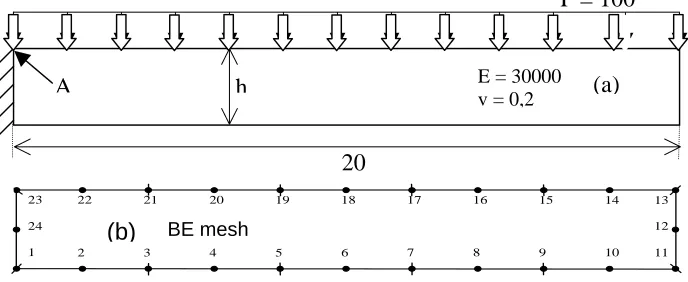
Example-1: This example deals with a cantilever beam of rectangular cross-section, unity thickness, and a variable height. The beam is under a distributed load of 100kgf/cm as shown in Fig.5. The goal is to obtain the beam height "h" such that the maximum stress at point A is at the yield stress fy=2500kgf/cm2. The modulus of
elasticity and Poisson’s ratio are in Fig.3. Using simple calculation from Strength of Materials we know that h=6.9282cm when the maximum stress, fy, is reached at point A of the fixed support. In this case, the objective
function may be taken as F=σ(h)-fy. Where σ(h) is the bending stress at point A which is a function of the
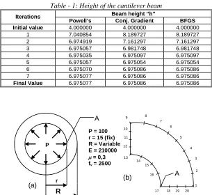
height "h". Fig.3(a) shows the beam and Fig.3(b) the BE mesh with 24 nodes corresponding to 12 quadratic elements. The results of the present formulation are reported in Table-1 for the three optimization methods used. The design variable is v = {h}. The initial value for the design variable is h=4. Convergence was attained in few iterations for each method as reported in Table-1.
1
12 24
23 22 21 20 19 18 17 16 15 14 13
11 10 9
8 7 6 5 4 3 2 A
P = 100
E = 30000 v = 0,2
(a)
A
h
20
(b)
BE meshFig. 3 - Cantilever beam for optimization of height
The final results, from all the three methods, correspond to the expected theoretical value. The expected h=6.9282cm is slightly different of the final values reported in Table-1. It’s because the BEM is more exact and based in the Theory of Elasticity and takes into account shear effects. The expected value of ‘h’ from the Strength of Materials formula is a simplification of the theory of elasticity.
Example-2: In this example, we want to get the minimum allowable thickness "t" of the pipe cross-section pictured in Fig.4(a). The pipe is under internal pressure "P". The inner radius "r" of the pipe is kept constant for flow reasons while the external radius "R" may vary. "R" is the design variable v = {R}. The thickness "t" is expressed as t=(R-r). Fig.4(a) and (b) show details of the pipe and the corresponding BE mesh discretization of one-quarter of the cross-section. 10 quadratic boundary elements with a total of 20 nodes are used for the BE mesh. From the theory of elasticity, the max hoop stress σθtakes place at the internal circumference, point A in
Fig.(4). The simple test is to find the thickness such that σθ, with a certain safe margin, is less than an allowable
stress. The allowable stress is defined as the yield stress fy/SF at point A. SF is the safety factor, here 1.5. The
objective function can be written as F=σθ(R)-fy/SF. The values of R, obtained from the present formulation,
are reported in Table-2 for the case of an initial value of R = 19cm.
For this example, P=100, r=15, the allowable fy/SF=2500/1.5=1666.7, and the final expected R is 15.9287cm - since from the theory of elasticity (Shames, 1964), σθ=P(R2+r2)/(R2-r2). The expected value for the thickness
Table - 1: Height of the cantilever beam
Beam height “h” Iterations
Powell’s Conj. Gradient BFGS Initial value 4.000000 4.000000 4.000000
1 7.040854 8.189727 8.189727
2 6.974919 7.161297 7.161297
3 6.975057 6.981748 6.981748
4 6.975035 6.975097 6.975097
5 6.975057 6.975054 6.975054
6 6.975070 6.975086 6.975086
7 6.975077 6.975086 6.975086
Final Value 6.975077 6.975086 6.975086
r
R
P
A
A
1 3 5 7 9
11
13
15
17 19
2 4 6 8
10
12
14
16
18 20
P = 100 r = 15 (fix) R = Variable E = 210000
µ = 0,3 fy= 2500
(a)
(b)
Fig. 4 – a) pipe section and b) one-quarter mesh with BEs
Table - 2: Pipe thickness
External Radius R and objective function F
Powell’s Conjugate Gradient BFGS Number of
Iterations
R F R F R F
Initial Values 19 1235.78 19 1235.78 19 1235.78 1 15.93345 14.859353 15.93345 15.859353 15.96345 7.568588 2 15.92496 0.225751 15.92456 0.345751 15.92490 0.568755 3 15.92496 0.199015 15.92456 0.136790 15.92490 0.189678
4 --- --- 15.92454 0.128984 --- ---
Final 15.92496 0.199015 15.92454 0.128984 15.92490 0.189678 T = R-r 0.92496 --- 0.92454 --- 0.92490 ---
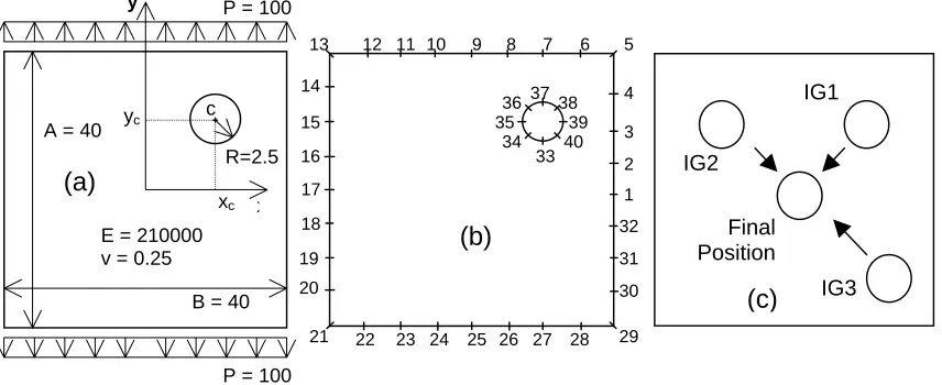
Example-3: In this application, the goal is to place a hole of radius “R” inside a panel such that the stress at the boundary of the hole is minimized. The panel is under traction as can be seen in Fig.5(a). The design variables, in this case, are the coordinates xc and yc of the center of the hole, v = {xc, yc}. Now, we deal with two
degrees of freedom. The objective function is defined as the Euclidean Norm of the principal stresses at the border of the hole. To minimize the Euclidean Norm of principal stresses is the same as to minimize the sum of the squares of the principal stresses, which are computed at the nodes of the BE elements defining the border of the hole as is expressed by Eq.(30).
F =
∑
(
)
=+
NF
NI j
j j
2 2 2
1
σ
σ
(30)where: σ1j and σ2j are the principal stresses at node number j with NI=33 and NF=40. Nodes 1 to 32 discretize
number of iterations. Practically, in the first iteration, the center of the hole moves to the expected solution (0, 0) - center of the panel, as shown in Fig.5(c). This example also tried different initial guesses, IGs; however, the final solution was always extremely close to the center of the panel, as expected - see Fig.5(c). In all the cases, the center of the hole was immediately reached soon after the first iteration and the final solution very close to the expected position (0, 0).
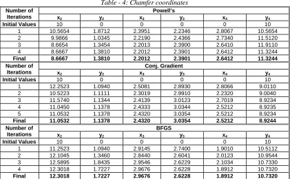
Example-4: Another application of the proposed formulation is to find a “smoother” configuration for a chamfer or notch as shown in Fig.6(a). The chamfer may change as indicated in the nodes in Fig.6(b). The final geometric shape of the chamfer takes into account the minimization of the principal stresses calculated at specific internal points as drawn in Fig.6(a). The discretization with BE is presented in Fig.6(b). The objective function, in terms of the principal stresses, is the same as Eq.(30) but, in this case, NI = internal point #1 and NF = internal point #6. The six internal points are depicted in Fig.6(a). In this case, the designvariables are v = {x2,
y2, x3, y3, x4, y4} which correspond to the coordinates of the nodal points 2, 3, and 4 – see Fig.6(b). Table-4 and
Fig.6(c) depict the results of this optimization. The values of the coordinate (x,y) of the nodal points are according to the Cartesian axis shown in Fig.6(a). All methods converged within a few numbers of iteration presenting similar results. For different referential points, stress components, or stress combination in the objective function, different chamfer profiles are obtained.
(c)
(b)
(a)
Final Position
IG3 IG2
IG1
R=2.5
E = 210000 v = 0.25
yc
xc
c
P = 100
B = 40 A = 40
y
x
38 39 40 37
34 35
36
33
32
31
30
29 5
4
3
2 1
28 27 26 25 24 22 23 21
20 19 18 17 16 15 14
13 12 11 10 9 8 7 6
P = 100
Fig. 5 - a) Initial position of hole. b) BE mesh. c) Result for various IGs
Table - 3: Location of a hole inside the Panel
Determination of the Hole Coordinates xc e yc for a fix Radius
Powell’s Conj. Gradient BFGS Number of
Iterations
xc yc xc yc xc yc
Initial Values 10 10 10 10 10 10
1 -0.011403 -0.006781 0.031983 -0.010543 -0.01753 0.00227
2 -0.001854 0.001977 0.004353 -0.00235 0.00146 0.00034
3 0.000651 -0.0009 0.00234 0.00341 0.00636 -0.00141
4 --- --- --- --- 0.00465 -0.00675
Final 0.000651 -0.0009 0.00234 0.00341 0.00465 -0.00675
6. CONCLUSIONS
variables always inside the feasible domain. The examples presented here are based on the minimization of stresses on few referential points. Those points could be inside or at the border of the structural member. The formulation is also reliable for other minimization quantities like, strains or displacements included in the objective function. The number of design variables used in the examples presented varied from 1 to 6. Convergence was attained soon in all applications studied. The BEM showed good numerical stability, precision in the stress results, easy for mesh updates during shape changes, and reduced number of degrees of freedom. The formulation proposed in this article, for the shape optimization of 2D continuous structures, shows good potential for simple applications.
100
1 2 3 4
hamfer
5 6
7
8
9
10
11
12 13 14 15
16
8 elements
0 5 10 15 20
0 10 X 20
Y
Final Positions
(c
Powell's
C.G.
BFGS
A = 20
Chamfer to design Internal
points where stresses are calculated
(b)
y100 x
(a)
Points to move todesign c
Points to move to design
chamfer ………
H=40 B = 20
L=40
Fig. 6: Design of a chamfer based on the stresses at internalreference points
Table - 4: Chamfer coordinates
Powell’s Number of
Iterations x2 y2 x3 y3 x4 y4
Initial Values 10 0 0 0 0 10
1 10.5654 1.8712 2.3951 2.2346 2.8067 10.5654
2 9.9866 1.0345 2.2190 2.4366 2.7340 11.5120
3 8.6654 1.3454 2.2013 2.3900 2.6410 11.9110
4 8.6667 1.3810 2.2012 2.3901 2.6412 11.3244
Final 8.6667 1.3810 2.2012 2.3901 2.6412 11.3244 Conj. Gradient
Number of
Iterations x2 y2 x3 y3 x4 y4
Initial Values 10 0 0 0 0 10
1 12.2523 1.0940 2.5081 2.8930 2.8066 9.0110
2 10.5223 1.1111 2.3019 2.9910 2.2320 9.0040
3 11.5740 1.1344 2.4139 3.0123 2.7019 8.9234
4 11.0450 1.1378 2.4333 3.0344 2.5212 8.9235
5 11.0532 1.1378 2.4320 3.0354 2.5212 8.9234
Final 11.0532 1.1378 2.4320 3.0354 2.5212 8.9244 BFGS
Number of
Iterations x2 y2 x3 y3 x4 y4
Initial Values 10 0 0 0 0 10
1 11.2523 1.0940 2.9145 2.7400 1.9010 10.5112
2 12.1045 1.3460 2.8440 2.6041 2.0123 10.9544
3 12.5895 1.8435 2.9546 2.6229 2.1034 10.7330
4 12.3018 1.7227 2.9676 2.6228 1.8912 10.7320
Acknowledgements
This article is part of a research in progress at University of Brasilia. The authors want to express their gratitude to CNPq (The Brazilian National Council for Scientific and Technological Development) and to CAPES (The Brazilian Committee for Postgraduate Courses in Higher Education) for the financial supports received for the development of these studies.
REFERENCES
Ricketts, R.E.; Zienkiewicz, O.C. (1984) “Shape Optimization of Continuum Structures”.In: New Directions in Optimum Structural Design. Ed.: E. Atrek, R.H.Gallagher, K.M.Ragsdeil, e O.C.Zienkiewicz; Wiley & Sons Ltd.
Fox, R.L. (1973) “Optimization Method for Engineering Design”. Massachusetts: Addison-Wesley. Gill, P.E.; Murray, W., Wright, M.H. (1981) “Practical Optimization”. London: Academic Press Inc.
Press, W.H.; Flannery, B.P.; Teukolsky, S.A.; Vetterling, W.T. (1986) “Numerical Recipes”. New York: Cambridge University Press.
Reklaitis, G.V.; Ravindran, A.; Ragsdell, K.M. (1983) “Engineering Optimization Methods and applications”. New York: Wiley.
Gallager R. H.; O. C. Zienkiewicz. (1973) “Optimum Structural Design: Theory And Applications”. London: John Willey.
Brebbia, C. A., Dominguez, J. (1989) “Boundary Elements: An Introductory Course”,Computational Mechanics Publications, McGraw-Hill, U.K.
Mota Soares, C. A.; Rodrigues, H. C. and K. K. Choi. (1984) “Shape optimal structural design using boundary elements and minimum compliance techniques”. ASME J of Mechanisms Tran. & Aut. in Design, V.106.
Banerjee, P.K.; Butterfield, R. (1981) “Boundary Element Methods in Engineering Science”. London: McGraw-Hill.