Analysis of the de-orbiting and re-entry of space objects with high area to mass ratio

Analysis of the de-orbiting and re-entry of space

objects with high area to mass ratio

Massimiliano Vasile

Edmondo Minisci

University of Strathclyde, Glasgow, UK

Romain Serra

University of Strathclyde, Glasgow, UK

James Beck

Belstead Research Limited, Ashford, Kent, UK

Ian Holbrough

Belstead Research Limited, Ashford, Kent, UK

This paper presents a preliminary analysis of the de-orbiting and re-entry dynamics of space objects with a large area to mass ratio. Two different classes of objects are considered: fragments of satellites (like solar panels and pieces of thermal blankets) and complete nano-satellites with passive de-orbiting devices like a drag sail. Different sources of uncertainty are considered including atmospheric density variability with latitude and solar cycles, aerodynamic properties of the object, light pressure, initial conditions. The coupling of the uncertainty in the aerodynamic forces and attitude motion is investigated to understand if low fidelity three degrees of freedom models can be used in place of more expensive high fidelity models to make predictions on the re-entry time. Modern uncertainty propagation and quantification tools are used to assess the effect of uncertainty on the re-entry time and study the dependency on a number of key parameters.

Nomenclature

a Semi-major axis, km

i Inclination, deg

α Angle of attack, deg

β Sideslip angle, deg

m Spacecraft mass, kg

A Cross-sectional area, m2 CD Drag coefficient,

-CR Radiation pressure coefficient,

-ρ Atmospheric density, kg/m3 F10.7 Solar flux, 10−22W/m2/s Kp Geomagnetic index,

-r Position, m

v Velocity, m/s

I.

Introduction

There are large uncertainties in the current state of knowledge of the upper atmosphere. This is a major contributor to the difficulties in the prediction of the re-entry of space debris into the atmosphere. Beyond

∗_{Professor, 75 Montrose Street.} †_{Lecturer, 75 Montrose Street.}

this, the aerodynamic behavior of objects between 120km and 300km altitude is not well researched, and the interaction between the aerodynamics and other forces perturbing the orbits are not well understood. With recent guidelines requiring that re-entry of satellites occurs within 25 years of the end-of-life, there have been a number of developments of area augmentation devices, designed to increase the area-to-mass ratio of the satellite thereby promoting orbital decay and decreasing the time to re-entry. Claims as to the effectiveness of a drag sail vary wildly, from figures assuming that the system is stable in the optimum orientation to assumptions of random tumbling.1 _{Within the literature, only one source investigating the}

attitude behavior of a drag sail has been found, which claims that non-planar sails have reasonably good stability characteristics.2 _{This investigation, however, considered the drag force in isolation, even at altitudes}

at which it is not the dominant orbital perturbation. Interaction of the drag with other perturbations, such as non-spherical gravity terms and gravity gradient effects does not appear to have been investigated. Improved understanding of the attitude motion of such sails can lead to improvements in design, or recommendations for particular design features to improve their effectiveness. A coupled model is, therefore, required to fully understand the dynamics of high area to mass ratio objects.

On the other hand a higher fidelity six degrees of freedom model is considerably more computationally expensive than a lower fidelity three degrees of freedom model. Therefore, it would be interesting to model the uncertainty introduced by a lower fidelity model in order to make acceptable predictions without a full high fidelity simulation. Furthermore, it is useful to study the uncertainty in the dynamic behavior of satellites with high area to mass ratio devices and of fragments with equal area to mass ratio, in order to derive a possible scaling law that allows for deriving similar predictions in both cases.

This paper will present an investigation of the dual uncertainties of the atmosphere and the attitude motion of a high area-to-mass ratio nano-satellites and of fragments or parts of satellites. An aerodynamic database for a range of designs and configurations is generated using DSMC calculations. Then, the effect of different parameters, characterizing the atmospheric drag, on the re-entry time is studied. This will provide an improved understanding of the basic motion and on how the attitude configuration combined with the variability in the atmospheric density can affect the re-entry. Modern uncertainty quantification techniques will be applied to these simulations in order to characterize the uncertainties on the re-entry time.

II.

Orbit propagation

In this work, two different simulators have been used: a 3 degrees of freedom (DoF) propagator, developed at the University of Strathclyde to study the re-entry of debris with high area-to-mass ratios, and a 6DoF one developed at Belstead Research Limited (BRL), that is used here to analyze the behavior of nanosatellites with area-augmentation devices. Note that BRL’s simulator, referred to as the ATS6, is also capable of 3DoF propagation in a simpler version named ATS3. A description of the two models follows.

A. 3DoF propagator

The orbit propagator at Strathclyde University is implemented in C++ and is primarily based on Mon-tenbruck & Gill.3 _{The state vector is composed of the Cartesian coordinates for position and velocity in an}

inertial frame. Integration is performed using a Runge-Kutta-Fehlberg 4(5) scheme, which features step-size control. As far as gravitational forces are concerned, the geopotential is expanded up to order and degree 9 and lunisolar perturbations are computed using low-precision ephemerides for the Sun and the Moon. As for the non-gravitational contributions, the atmospheric densityρis computed with the Jacchia-Gill model.4

Apart from the positions of both the object and the Sun, two other parameters determine its value: the mean solar fluxF10.7, given in units of 10−22W/m2/s, and the geomagnetic indexKp, measured on a scale from 0

to 9. These two quantities normally change with time on various scales. For instance, long term variations are correlated to solar cycles. However, here, they are assumed to be constant during each propagation. Their range of variability is explored via the uncertainty quantification technique described in Section III. For this study, predicted monthly averaged values5_forF

1. Non-gravitational forces for a spherical object

Letmdenote the mass of the spacecraft, which is assumed to be constant over time. The acceleration due to drag ¨rdrag is:

¨rdrag=−

1 2CD

A

mρkvrelkvrel (1)

where the parameters are:

• A: cross-sectional area

• CD: drag coefficient

• vrel: relative velocity with respect to the flow

The cross-section area is fixed for a given spherical object while the drag coefficient is assumed to remain constant with time for a given trajectory, but a range of possible values is investigated via the Uncertainty Quantification technique described in Section III to try to capture the dependency on the average tumbling motion. Finally, the atmosphere is assumed to rotate with the Earth. The other non-gravitational force investigated for a spherical object is the solar radiation pressure. In order to see the effects of the worst-case scenario, no eclipse is taken into account. As a result, the corresponding acceleration ¨rSRP writes:

¨

rSRP=− A mPSun

AU2

krSunk3

rSun (2)

where the parameters, not yet introduced, are:

• AU: astronomical unit

• rSun: Sun’s position (computed from ephemerides)

• PSun= 4.560×10−6N/m2: solar radiation pressure in the vicinity of the Earth

It is worth noticing that the two non-gravitational accelerations are both proportional to the area-to-mass ratioA/m, while gravitational contributions are independent of mass. However, for relatively low altitudes, as the ones considered in this paper, the acceleration due to drag is several orders of magnitude higher than radiation pressure and drives the orbit decay.

2. Extension to a square flat plate

For an ideal spherical object, there is no dependency of the orbital motion on attitude. Therefore, in order to study the potential effects of non randomly tumbling objects, a square flat plate is considered. Strictly speaking, a 6DoF simulation would be required for different geometries, and aerodynamic forces would need to be derived for each orientation, Mach number and altitude. As a first analysis, in this paper, we will assume that the attitude is maintained constant through the whole trajectory and we calculate the aerodynamic forces for a discrete number of configurations. The drag coefficient CD is computed as a function of the

side-slip angleβ and the angle of attack α. More precisely, reference values are obtained for a few specific orientations via Direct Simulations Monte Carlo (DSMC) and an interpolated model is then used to estimate

CDfor any possible orientation. The methodology adopted for the DSMC is detailed in the next paragraph.

The dsmcFoamStrath6 _{code was used to run simulations of the square flat plate, based on the openFoam}

platform. A Variable Hard Sphere (VHS) model was used, along with a fully diffusive reflection model. The good DSMC practice suggests using a mesh refinement determined by the Mean Free Path (MFP). The maximum cell size has to be less than 1/3 of the MFP. In this work, the free molecular regime has been investigated. In this particular flow regime, the cell size is dictated by the geometrys surface quality achievable with the meshing tool. A meshing box of 3x2x2 [m] has been used, with a free flow cell size of 8.6cm, the minimum cell size on the flat plate surface was 0.5cm. The mesh was filled with 20 particles per cell, granting a good precision (the recommended is 10 particles per cell). The DSMC timestep was 10−5_{, the}

50km steps. The flat plate relative velocity was computed by the orbital velocity, with the assumption of a circular orbit. The molecular composition, density, and temperature were acquired by the MSISE00 model embedded in Matlab. The wall temperature used for the Gas surface interaction was set toTwall= 350K, the

flow temperature changes over the altitude. The speed ratio changes over the altitude due to the variation in the molecular composition and the free flow temperature. The flow velocity has the same direction and orientation of the X-axis (e.g.: V = [7814.1 0 0]m/s). The reference system is shown in Figure 1 along with the configuration where both angles are zero. In Figure 2 the sideslip is achieved by a rotation of 45 degrees about the Y axis, and the angle of attack is zero. The rotation order is always the same: first rotation about the Y axis, second rotation about the Z axis. Results are given in Table 2. Note that for the particular cases whereβ = 0, the outputs are in good agreement with the literature.7

Table 1. Drag coefficient,CD, from the DSMC

a a a a a a a a a aa Altitude (km)

(β, α)

deg (0,0) (45,0) (0,45) (90,0) (45,45) (90,45)

150 2.105 1.479 1.480 0.122 1.051 0.129

200 2.127 1.493 1.496 0.141 1.057 0.148 250 2.138 1.500 1.501 0.153 1.062 0.160

300 2.146 1.505 1.506 0.160 1.065 0.166 350 2.153 1.508 1.508 0.164 1.068 0.172

400 2.155 1.511 1.511 0.168 1.066 0.175

From Table 2, average values forCD over the altitude range are obtained for each occurrence of (β, α).

Due to the symmetry of the square plate, only values in [0,90]2degrees are required. Moreover, some cases can be immediately deduced from the available data e.g. (0,90) is similar to (90,0). In the end, nine different configurations are used as references to compute an interpolated model of log₂(CD(β, α)). It consists of a

second order polynomial fit obtained in Matlab. As a result, theCDis a non-linear function of (β, α). Hence

a uniform sampling of these two angles via the Uncertainty Quantification technique described in Section III would lead to a non-uniform distribution of the drag coefficient.

B. ATS3 and 6

BRL’s ATS6 (respectively ATS3) is a 6DoF (respectively 3DoF) aerothermodynamic trajectory simulator that embodies the work of Gainer & Hoffman.8 _{Fundamental equations are written in an Earth-fixed reference}

frame and attitude is represented using quaternions. Drag is evaluated from a database of coefficients pre-calculated for a number of speed ratios in the range 2 - 25, for all orientations of the geometry relative to the flow in steps of 5 degrees of attack and sideslip. The required values for intermediate attitude and velocities interpolated in three dimensions (velocity, attack, sideslip). The aerodynamic databases themselves are constructed from an in-house aerothermodynamic coefficient generator (ACG). This employs a ray-tracing scheme to evaluate the profile of the geometry being examined from either geometric primitives, or, as in this case, an STL CAD file. Continuum drag coefficients are generated using modified Newtonian theory. Free molecular coefficients are constructed from shear and pressure terms as described by Chambre & Schaaf.9

Figure 1. Reference system and geometrical configuration for the case(β, α) = (0,0)degrees of the DSMC

III.

Uncertainty Analysis

A non-intrusive technique is used to fast propagate uncertainty during deorbit and re-entry: it consists in a Chebyshev high order polynomial approximation that is briefly described in this Section. The reader can refer to Tardioli et al.10 _{for more details on this method. The non-intrusive Chebyshev approach is}

a polynomial approximation of the function of interest. More precisely, the latter is interpolated with a multivariate Chebyshev polynomial via a Latin hypercube sampling of the model. Letnbe the number of variables anddthe desired degree of interpolation. The corresponding Chebyshev basis is:

Ci(x) =

d

Y

r=1

Cir(xr),

where C0(xr) := 1, Cir(xr) := cos(irarccos(xr)) andx∈[−1,1]

d_{. The fact that Chebyshev polynomials}

are defined on the unit hypercube requires to translate the original variables in this particular set. The generic polynomial interpolant for the function of interest has the form

F(x) = X

i,|i|≤n

piCi(x),

wherepiare the unknown coefficients to be computed from the samples. The minimum number of required

nodes is equal to the size of the Chebyshev basis:

N = (n+d)!

d!n! (3)

When the number of samples equals this value, the coefficients of the Chebyshev polynomial are obtained by inverting the following linear system of equations:



  

C0(x0,1) . . . CN(x0,1)

..

. . .. ...

C0(x0,s) . . . CN(x0,s)

    ·     p0 .. . pN     =     y1 .. . ys    

wheresis the number of grid points andy1, . . . , ysare the true values at these points obtained by evaluating

the real model. When more samples are computed i.e. s >N, a least square approach enables to compute the coefficients. This adds more robustness to the method.

IV.

Results and analysis

A. Study of the re-entry of debris with high-area to mass ratio

In this section we will investigate the effect of uncertainty in the atmospheric density, drag coefficient, light pressure and area to mass ratio on the re-entry time of fragments of satellites with high area to mass ratio. We consider two cases: one in which the object is randomly tumbling and its average drag coefficient is equivalent to that of a sphere (sphere case), the other in which the object is assumed to take a semi-stable configuration (flat plate case).

1. Case of spherical debris

In this part, the atmospheric re-entry of spherical debris with high area-to-mass ratios has been investigated. The idea is to study on a range of orbits the behavior of a cloud of fragments as obtained for example after a collision. For this analysis, the propagation is stopped as soon as the simulated object reaches an altitude below 120km. The initial epoch was chosen as January 1st 2024 12:00 UTC, due to predictions5 _foreseeing

coefficient as well as all the angles among the Keplerian orbital elements. As for the area-to-mass ratio, it covers two orders of magnitude: from 1 (similar for example to a solar panel) to 10 (similar for instance to a piece of blanket or paint). Finally, values for the drag coefficient spread over ±10% around a nominal value of 2. Based on the aforementioned re-entry criterion, a surrogate has been computed for the re-entry time. Due to the large span of final values, it is actually the logarithm of the number of days before re-entry that has been approximated with a 5-th order Chebyshev polynomial. For the sake of robustness, it was interpolated on a wider range than the one actually used in the analysis, hence the bracketed values for some parameters in Table 2.

Table 2. Ranges of parameters for the sphere (numbers under brackets are the ones used for the original Chebyshev interpolation as the analysis was performed on a narrower range)

Number Name Unit Min. value Max. value

1 Semi-major axis km (6650) 6700 (7150) 7100

2 Eccentricity - 0 0.01

3 Inclination deg 0 180

4 Right ascension of the ascending node deg 0 360

5 Argument of perigee deg 0 360

6 True anomaly deg 0 360

7 Area-to-mass ratio m2_{/ kg 1 10}

8 Mean solar flux 10−22_W/m2_{/s (90) 100 (210) 200}

9 Geomagnetic index - (2) 2.33 (4) 3.66

10 Drag coefficient - (1.5) 1.8 (2.5) 2.2

11 Radiation pressure coefficient - 1 2

In the following, some analysis is performed on the real model first, before using the surrogate to compute re-entry probabilities.

Figure 3 shows the re-entry time as a function of semi-major axisaand inclinationifor a particular value of the other parameters. For each point on the (a, i) grid, a full propagation was run to compute re-entry time with all other parameters set to mid-range values from Table 2. For instance, the drag coefficient is equal to 2. Some fairly intuitive trends can be seen on this map. First of all, the larger the semi-major axis is, the longer the time of re-entry is, simply because the initial altitude is higher. Second, orbits with a near-polar inclination lead to slower re-entry compared to near-equatorial ones. This is due to the Earth’s oblateness that implies higher altitudes at higher latitudes and thus less drag. Lastly, retrograde orbits decay faster than prograde orbits as the former go in a direction opposite to the rotating atmosphere.

Figure 3. Days before re-entry for middle-range values from Table 2 as a function of initial semi-major axis and inclination (logarithmic scale)

Next, the surrogate is used to obtain various statistics on re-entry, assuming uniform sampling of the ranges of values in Table 2. The relative fast evaluation of the Chebyshev polynomial allows for a fairly large number of samples (here 105_{) to estimate the probability of re-entry. The following studies have been carried}

out as a function of the initial semi-major axis and/or inclination, as these two parameters can describe any near-circular orbit in a rather general way. For individual studies,aor i is discretized on one axis and the other 10 parameters are free. For coupled studies, the plane is divided into a grid and for each occurrence of (a, i), the 9 other parameters are sampled.

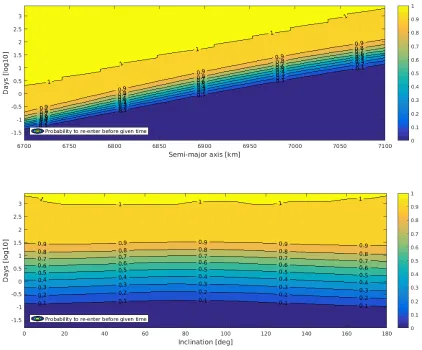
In Figure 6, marginal cumulative distributions both for the initial semi-major axis and the initial in-clination are shown. In other words, it shows the probability to re-enter within the time on the vertical axis depending on the quantity on the horizontal axis. It can be seen that the final range for re-entry is approximately from 0.1 to 1000 days, covering a total of 4 orders of magnitude. This demonstrates a large variability with respect to Figure 3, especially for the maximum values. The same trends already discussed appear again: slow re-entry is more likely to happen for large values ofaas well as for near-polar orbits (i

Figure 4. Days before re-entry for middle-range values from Table 2 and initial inclination of 10deg as a function of initial ascension of the ascending node and argument of perigee (logarithmic scale)

Figure 7. Probabilities to re-enter before given time as a function of initial semi-major axis and inclination from surrogate for the sphere

2. Case of a square flat plate

This part of the study uses a 3DoF model to approximate the motion of a square flat plate, as described in Section II. Similarly to the spherical case, orbit propagation is stopped when altitude reaches 120km and the initial epoch is 01/01/2024 at midday. A 5-th order Chebyshev polynomial has been computed as a surrogate for the logarithm of the re-entry time, using the ranges reported in Table 3. While the study of spherical debris simulated a large range of area-to-mass ratio as in a cloud of fragments, here A/m is concentrated around 1, focusing on a particular type of plate similar to a piece of solar panel. The study is still restricted to near-circular orbits. In accordance with the available data from the DSMC, the initial possible altitudes are lower than for the spherical case: from around 200 to 500km. Moreover, from the previous analysis we can say that the the dynamics is mainly governed by gravity and aerodynamics, therefore solar radiation pressure is not included in the simulations in this section.

The key simplifying assumption in this analysis is that the flat plate maintains its orientation with respect to the velocity vector during the whole deorbiting trajectory. This is an extreme case that is not true in general as it will be demonstrated in section 2. Under this assumption the flat plate rotates, as it moves along the trajectory, to maintain its orientation with respect to the local velocity vector.

Table 3. Ranges of parameters for the square flat plate

Number Name Unit Min. value Max. value

1 Semi-major axis km 6600 6800

2 Eccentricity - 0 0.01

3 Inclination deg 0 180

4 Right ascension of the ascending node deg 0 360

5 Argument of perigee deg 0 360

6 True anomaly deg 0 360

7 Area-to-mass ratio m2_{/ kg 0.9 1.1}

8 Mean solar flux 10−22W/m2/s 100 200

9 Geomagnetic index - 2.66 3.33

10 Sideslip angle deg 0 90

11 Angle of attack deg 0 90

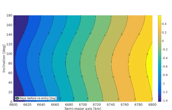
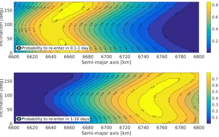
As before, the time of re-entry is calculated as a function of initial semi-major axis and initial inclination accounting for uncertainty in all the other parameters. The results from the evaluation of the real model on mid-range values from Table 3 are shown in Figure 9. The map demonstrates the same trend as for the spherical case. For example, initial inclinations around 0 or 180 degrees lead to faster re-entry than inclinations around 90deg.

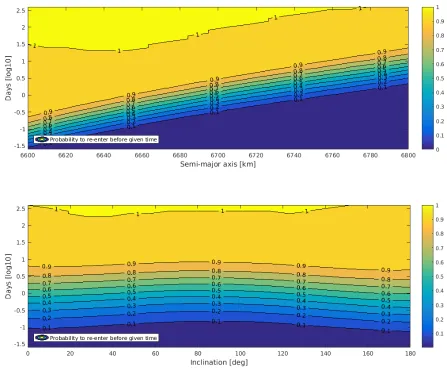
A statistical analysis of re-entry is presented next, using the surrogate and uniform Monte Carlo simu-lations with 105_{samples (as for the sphere). Figure 10 shows the marginal cumulative distribution both for}

the semi-major axis and the inclination. Overall, the re-entry range proves to be around 0.05-500 days. It is almost as spread out as for the sphere, even though the range of initial semi-major axis contains lower values. This illustrates the dependency of drag on attitude for a non-tumbling object. Two different aerody-namic configurations can produce drastically different values for theCD, resulting in quite different re-entry

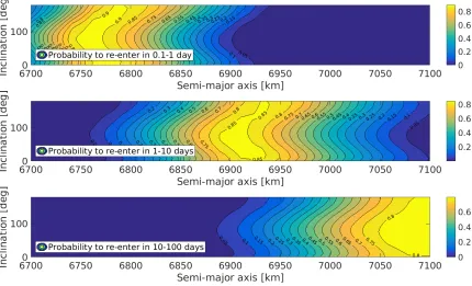
times. Once again, the variability tends to be more pronounced for maximums rather than for minimums. Probabilities to re-enter within various times and intervals are shown respectively in Figure 11 and Figure 12.

Figure 11. Probabilities to re-enter within given time as a function of initial semi-major axis and inclination from surrogate for the plate

3. Comparison between a sphere and a square flat plate with similar area-to-mass ratio

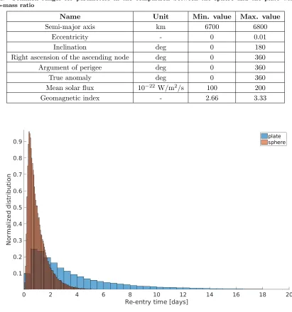
In order to isolate the effect of a fixed attitude on drag, the differences on re-entry time between a spherical object and a square flat plate of similar dimensions (namely a unit area-to-mass ratio) have been investigated. This comparison has been obtained from their respective surrogates previously computed. For consistency, the parameters are sampled on a common range - when relevant - reported in Table 4. In particular, the span of initial altitude is approximately 300-500km. The corresponding distributions can be seen in Figure 13, even though the tail for the flat plate actually spreads well over 20 days and has been cut off here. In fact, due to the many possible aerodynamic configurations for the plate, there is a higher variability inCD

than for the sphere. This results in a re-entry range for the plate that is much larger especially in the upper end (100 days against 10).

Table 4. Common ranges for parameters in the comparison between the sphere and the plate with unit area-to-mass ratio

Name Unit Min. value Max. value

Semi-major axis km 6700 6800

Eccentricity - 0 0.01

Inclination deg 0 180

Right ascension of the ascending node deg 0 360

Argument of perigee deg 0 360

True anomaly deg 0 360

Mean solar flux 10−22_W/m2_{/s 100 200}

Geomagnetic index - 2.66 3.33

B. Study of aerodynamic stability for drag sails

This section will investigate the motion of a nano-satellite equipped with a passive de-orbiting device such a drag sail. The interest is to identify the effect of stability in the attitude motion on the re-entry time and how the predictions with a full 6dof simulation differs from a simpler 3dof simulation. This section will also look into how the area to mass ratio affects the attitude motion, for different configurations, and therefore, the re-entry time.

1. De-orbit drag sail configuration

The test cases for drag sails are based on available data for the SSTL TechDemoSat mission with the Cranfield University Icarus drag sail. It is worth noting that the de-orbit predictions of this drag augmented system are based on the assumption that the system is randomly tumbling,11 _{and de-orbit from an initial altitude}

of 635km on a sun-synchronous orbit is expected to take just under nine years.

The basic geometry of the satellite is that of a 77cm x 50cm x 90cm cuboid. The launch adaptor interface is on the -Y face, which suggests that the center-of-mass is below center. As no precise mass properties are available the sensitivity of the drag sail stability to an offset in the center-of-gravity from the geometric center requires analysis. The satellite mass is approximately 150kg, and the sail construction is about 3.5kg. In the deployed configuration the sail has a small sail-angle of 8deg (see Fig. 14). It is worth noting that further sails from Cranfield11have been designed flat (0deg angle to the vertical), which is relatively common amongst drag sails. Therefore, a base test case with a flat configuration drag sail is considered.

It is worth noting that there are other configurations of drag sail which have been considered in the literature. Roberts & Harkness2 consider a conical sail with an apex angle of approximately 45deg and claim that this configuration is aerodynamically stable, due to the center-of-pressure being moved backward relative to the center-of-gravity. Interestingly, this is in contrast to the tumbling assumption of Kingston et al.,11 _{and is worthy of investigation. No attempt to determine if a stable configuration can be established}

from a tumbling state has been made in either case. They also state that both gravity gradient perturbations and solar radiation pressure effects are low at the conditions of interest. Therefore, a second configuration of drag sail using an angle is proposed. Rather than using a cone, the more practical solution of an Icarus-type sail with a larger angle to the vertical is suggested. The geometry remains as before, with the sail in four segments, but with a larger angle to the vertical.

To assess the performance of the drag sail, a test spacecraft is used. This is based on the TechDemoSat spacecraft with a simplified geometry and approximate mass as given in Table 5.

Table 5. General Spacecraft Properties

Attribute Value

Shape Cuboid

X-length (m) 0.5

Y-width (m) 0.77 Z-height (m) 0.9

Mass (kg) 150

To test different drag sail configurations, the sail size and sail angle are tested. Two sizes of sail, and two angles are used, with one condition where the projected area of the vehicle, and thus the expected drag when aligned, are identical. The parameters defining the sail geometry are given in Figure 14. The sail height is defined similarly to the sail width in the direction out of the page.

Using these parameters, four drag sails are defined. The first two have a different sail angle, but the same overall height and width as in the Figure 14 schematic. From this, it is clear that the nominal drag area is the same, but the area of the sail material is significantly different. Therefore, two further sails are defined, such that the effect of the sail angle on a drag sail of a fixed sail area, and thus fixed packing volume, can be seen. The four sails are defined in Table 6.

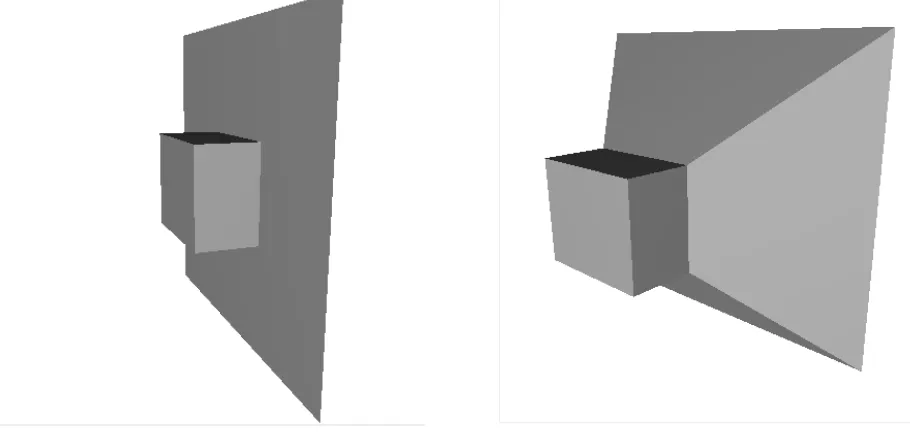
Figure 14. Sail geometry parameter definition

Table 6. Drag Sail Definitions

Drag Overall Overall Sail Height Sail Width Sail Angle Sail Height (m) Width (m) (m) (m) (degrees)

DS1 2.75 2.5 0.925 0.865 0

DS2 2.75 2.5 1.308 1.223 45

DS3 3.516 3.216 1.308 1.223 0

DS4 2.208 1.993 0.925 0.865 45

Table 7. Test cases

Test case Spacecraft center of gravity Drag sail Projected area (m2₎

1 (0,0,0) DS1 6.875

2 (0,0,0) DS2 6.875

3 (0,0,0) DS3 11.31

4 (0,0,0) DS4 4.40

Drag sails 1 and 2 are shown in Figure 15. Note that for consistency with the satellite drawings, the sail is on the +X side of the vehicle, so strictly, the stable position is flying backwards.

Figure 15. Drag sails 1 and 2

2. Aerodynamic stability

A preliminary investigation of the stability of the four vehicle geometries has been undertaken with ATS6. For this study the center of mass of the vehicle was placed at the geometric center of the cuboid section of the vehicle, and an inertia tensor constructed on the assumption that the vehicle is modeled as a uniform regular cuboid. An initial condition was taken from the TechDemoSat-1 Two Line Element (TLE) for 2016-07-27 published on CelesTrak, as extracted in Table 8.

Table 8. Orbital elements from TechDemoSat-1 TLE for 2016-07-27

Inclination RAAN Eccentricity Argument of Mean anomaly Mean motion (deg) (deg) (-) perigee (deg) (deg) (revolution / day)

98.3250 301.9984 0.0006960 43.8230 316.3533 14.81208499110957

This TLE results in the simulation initial condition described in Table 9. From this point a trajectory was propagated using a 4-th order Runge-Kutta integrator with a step size of 5 seconds.

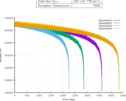
A dynamic Jacchia Roberts atmosphere model was employed with parameters as defined in Table 10. The initial pitch rate of -0.0618 degrees / second was empirically selected to maintain a zero angle of attack as the vehicle orbited. This is to ensure the correct pitch rate to maintain orientation relative to the wind as the vehicle orbits the planet. As can be seen in Figure 16, the four sail configurations under consideration result in re-entries between 6 and 12 years, well within the 25-year constraint.

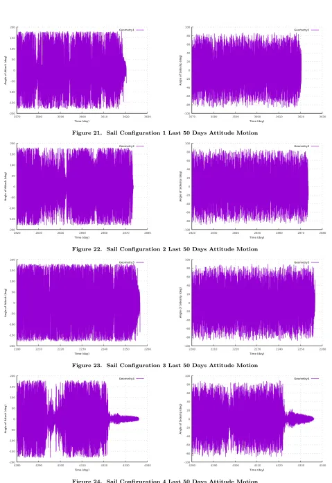
Examining the vehicle attitude in the first few days of the predicted trajectory, as shown in Figure 17 through Figure 20, although the initial condition has been selected to try to maintain a stable vehicle first attitude through the orbit the attitude motion very quickly degenerates to a tumbling motion, regardless of sail configuration.

Examining the full trajectories, it can also be seen that the amplitude of this motion does not fall. Further, as shown in Figure 21 through Figure 24, and in all but the case of geometry 4 stability is not regained prior to re-entry. In the case of geometry 4 tumbling stops approximately 10 days prior to re-entry at an altitude of 325km.

Table 9. ATS6 Trajectory Initial Conditions

Variable Day 2

Date / time (UTC) 2013-10-22 03:00

Latitude (degrees) 81.37

Longitude (degrees) 115.94

Altitude (m) 642886

Velocity (m/s) 7621.82

Bearing (degrees) 73.72

Flight Path Angle (degrees) 0.0419

Sideslip (degrees) 0

Bank (degrees) 0

Pitch rate (degrees / sec) -0.0618

Yaw rate (degrees / sec) 0

Roll rate (degrees / sec) 0

Table 10. Jacchia Roberts Atmosphere Properties

Variable Value

GeomagneticKp 3.22

Solar fluxF10.7 132×10−22W/m2/s

Exosphere Temperature 703K

Figure 17. Sail Configuration 1 First 2 Days Attitude Motion

Figure 18. Sail Configuration 2 First 2 Days Attitude Motion

Figure 19. Sail Configuration 3 First 2 Days Attitude Motion

Figure 21. Sail Configuration 1 Last 50 Days Attitude Motion

Figure 22. Sail Configuration 2 Last 50 Days Attitude Motion

Figure 23. Sail Configuration 3 Last 50 Days Attitude Motion

6DoF entry date is predicted to be slightly later than the equivalent tumble averaged 3DoF trajectory. This suggests that not only is the sail not being correctly oriented to the direction of travel in order to maximize the vehicles drag, but it fact it is failing to achieve the drag coefficient predicted by random tumbling, which is generally assumed in dragsail analysis to be a worst case. This analysis suggests that this assumption has not been justified.

Figure 25. Sail Configuration 1 3DoF / 6DoF Com-parison

Figure 26. Sail Configuration 2 3DoF / 6DoF Com-parison

Figure 27. Sail Configuration 3 3DoF / 6DoF Com-parison

Figure 28. Sail Configuration 4 3DoF / 6DoF Com-parison

These results would appear to contradict the work of Roberts & Harkness2 which suggests that conic sails should be stable at altitudes of 600km. However, it should be noted that sails examined by Roberts & Harkness are substantially larger relative to the mass of the vehicle at approximately∼1m2/kg, than those proposed here (∼0.05m2_{/kg). This will result in the substantially larger torques maintaining that attitude}

of the vehicle in its optimum orientation, although such large sails are beyond current boom manufacturing and sail packaging technology. If the sails in geometries 1 and 2 are scaled to give projected areas of 150m2

- named geometry 5 and 6 respectively; bringing the mass per unit projected area to∼1m2_{/kg the resulting}

attitude motion is summarized in Figure 29 and Figure 30. Whilst the flat sail of geometry 5 continues to show large amplitude motion, it does not break down into random tumbling. In contrast, the greater sail area (211m2_{) and higher average drag of the pyramid sail in geometry 6 leads to stable motion. In both}

instances re-entry is predicted in approximately than 90 days, indicating that the average drag experienced by the two geometries during re-entry is similar.

Even when the sail area is normalized to 150m2_{, with a resulting maximum projected area of 107m}2_,

Figure 29. Sail Geometry 1 Scaled to 150m2 Pro-jected Area Sideslip Profile

Figure 30. Sail Geometry 2 Scaled to 150m2 Pro-jected Area Sideslip Profile

Figure 31. Sail Geometry 1 Scaled to 150m2 Pro-jected Area Altitude Profile

Figure 32. Sail Geometry 2 Scaled to 150m2 Pro-jected Area Altitude Profile

Figure 33. Sail Geometry 2 Scaled to 150m2 _Sail Area Sideslip Profile

Figure 34. Sail Geometry 2 Scaled to 150m2 _Sail Area Altitude Profile

Table 11. Large Drag Sail Definitions

Drag Overall Overall Projected Sail Height Sail Width Sail Area Sail Angle Sail Height (m) Width (m) Area (m2_{) (m) (m) (m}2_{) (degrees)}

DS5 12.5 12 150 5.80 5.62 150 0

DS6 12.5 12 150 8.20 7.94 211 45

A first order analysis of the onset of tumbling may be undertaken by adjusting the mass and moment of inertia of a sail to obtain a suitable projected area to mass ratio. It should be noted that this approach employs the simplifying assumption that the mass of the sail is negligible relative to that of the vehicle, and therefore, adjusting the overall system mass has no effect on the center of mass. Figure 35 and Figure 36 illustrate the sideslip profiles for geometry 5 and 6 with masses adjusted to give area to mass ratios in the range 0.01m2_{/kg - 10m}2_/kg.

Figure 35. Sail Geometry 5 Sideslip Profile as a Function of Area:Mass

Figure 36. Sail Geometry 6 Sideslip Profile as a Function of Area:Mass

Tumbling occurs for area to mass ratios below 0.75m2_{/kg and 0.02m}2_{/kg for geometries 5 and 6}

respec-tively. As expected, the onset of tumbling is highly geometry specific. The assumption that the mass of the sail is negligible leads to the center of mass being located at the geometric center of the main vehicle for all configurations. Clearly, the 45deg sail angle and greater X component of geometry 6 leads to the center of pressure being further behind the center of gravity, resulting in a larger static margin and greater stability. The greater sail area of geometry 6 will also be contributing to the overall stability of this configuration, as is shown by an area to mass ratio of 0.05m2_{/kg tumbling when applied to geometry 7 in Figure 37. It should}

be noted that the smaller sail area in this instance will also result in the center of pressure being closer to the center of gravity, reducing the static margin of this configuration in comparison to geometry 6. As a consequence, the reduction in stability cannot be entirely attributed to the decreased sail area.

Further analysis is required to assess the limits of the sail area required to maintain stability for a given satellite mass when the simplify assumption of a negligible sail mass is removed.

In a similar manner a first order assessment of the impact of scale on stability given a constant area to mass ratio can be undertaken by scaling the mass and moment of inertia of geometry 5 and 6 to match the area to mass ratio of configurations 1 and 2 respectively. The results of this comparison are illustrated in the attitude motion of the vehicles as shown in Figure 38 and Figure 39.

The motion of sail configurations 1 and 5 when scaled to the same area to mass ratio initially show a good correlation. However, after half a day the predicted behavior diverges. It is speculated that this variation is caused by the fact that only the mass has been scaled and the relative sizes of the main vehicle have not been similarly treated. It should also be noted that attitude motion is sensitive to small differences in input, and that variations in predicted behaviors tend to be reinforced. Clearly, the behavior of geometries 2 and 6 differ significantly with configuration 6 displaying attitude motion with a small amplitude relative to that of geometry 2.

Figure 37. Sail Geometry 7 Sideslip Profile as a Function of Area:Mass

Figure 38. Constant Area To Mass Ratio Comparison, Geometries 1 and 5

Figure 40. First 80 days Sideslip Motion of Geom-etry 6 Constant Area to Mass Ratio

Figure 41. Full Sideslip Motion of Geometry 6 Constant Area to Mass Ratio

V.

Conclusions

The first part of this work investigated the re-entry time of fragments of satellites under uncertainty while the second part investigates the aerodynamic stability of drag sails for a nanosatellite. From the preliminary results in this paper one can say that where a high area-to-mass ratio object can expect some stability, it is a requirement that a 6DoF model is used in order to provide a good assessment of the de-orbit time. However, in cases that the object is expected to tumble, a 3DoF analysis using a tumble averaged drag provides a good baseline for an uncertainty analysis.

The uncertainty on the atmospheric drag up to an altitude of about 800km is greatly dominating the re-entry time with large variations in the probability of a successful re-entry. For the spherical case, a probability of 1 for a re-entry time of less than 10 days is expected for altitudes lower than about 500km. On the contrary the uncertainty on the configuration of the flat plate gives a probability of 1 only bellow 300km. These variations have an impact on the re-entry point and on the probability of a collision with other objects in orbit. The results with the flat plate need to be taken with care and only as limit cases. As demonstrated in the case of the drag sail some configurations are not necessarily stable and can induce a tumbling motion. Therefore, although all orientations were considered equally probable, in reality only some of them are actually possible. Therefore, additional work is required to analyze the 6DoF dynamics of the flat plate, for different geometries, and to include the uncertainties in the 6DoF propagation of the drag sail in order to investigate the scalability of the uncertainty on the re-entry time withA/m.

VI.

Acknowledgments

The Authors would like to thank the UK Space Agency for the grant supporting project DEUQ - ”Multi-fidelity analysis of space debris de-orbiting and re-entry under uncertainty” and the publication of this work. The Authors also wish to thank Alessandro Falchi at Strathclyde University for his help with the Direct Simulation Monte Carlo.

References

1_{Lappas, V., Pellegrino, S., Guenat, H., Straubel, M., Steyn, H., Kostopoulos, V., Sarris, E., Takinalp, O., Wokes, S., and}

Bonnema, A., “DEORBITSAIL: De-orbiting of satellites using solar sails,”Space Technology (ICST), 2011 2nd International Conference on, IEEE, 2011, pp. 1–3.

2_{E Roberts, P. C. and Harkness, P. G., “Drag sail for end-of-life disposal from low earth orbit,”Journal of Spacecraft and} Rockets, Vol. 44, No. 6, 2007, pp. 1195–1203.

3_{Montenbruck, O. and Gill, E.,Satellite orbits: models, methods and applications, Springer Science & Business Media,}

2012.

4_{Gill, E., “Smooth bi-polynominal interpolation of Jacchia 1971 atmospheric densities for efficient satellite drag}

computa-tion,” 1996.

5_{Flohrer, T., Krag, H., Lemmens, S., Bastida Virgili, B., Merz, K., and Klinkrad, H., “Influence of solar activity on}

6_{Scanlon, T., Roohi, E., White, C., Darbandi, M., and Reese, J., “An open source, parallel DSMC code for rarefied gas}

flows in arbitrary geometries,”Computers and Fluids, Vol. 39, No. 10, 2010, pp. 2078–2089.

7_{Dogra, V. K., Moss, J. N., and Price, J. M., “Rarefied flow past a flat plate at incidence,” 1988.}

8_{Gainer, T. G. and Hoffman, S., “Summary of transformation equations and equations of motion used in free flight and}

wind tunnel data reduction and analysis,” 1972.

9_{Schaaf, S. A. and Chambr´e, P. L.,Flow of rarefied gases, University Press, 1961.}

10_{Tardioli, C., Kubicek, M., Vasile, M., Minisci, E., and Riccardi, A., “Comparison of Non-Intrusive Approaches to}

Un-certainty Propagation in Orbital Mechanics,”Proc. of the AIAA-AAS Astrodynamics Specialists Conference, Veil, Colorado, USA, 2015.

11_{Kingston, J., Palla, C., Hobbs, S., and Longley, J., “Drag augmentation system modules for small satellites,” ESA Clean}