Nonlinear preconditioning : how to use a nonlinear Schwarz method to precondition Newton's method

NONLINEAR PRECONDITIONING: HOW TO USE A NONLINEAR

SCHWARZ METHOD TO PRECONDITION NEWTON’S METHOD

∗

V. DOLEAN†, M. J. GANDER‡, W. KHERIJI§, F. KWOK¶, AND R. MASSON§

Abstract. For linear problems, domain decomposition methods can be used directly as iterative solvers but also as preconditioners for Krylov methods. In practice, Krylov acceleration is almost always used, since the Krylov method finds a much better residual polynomial than the stationary iteration and thus converges much faster. We show in this paper that also for nonlinear problems, domain decomposition methods can be used either directly as iterative solvers or as preconditioners for Newton’s method. For the concrete case of the parallel Schwarz method, we show that we obtain a preconditioner we call RASPEN (restricted additive Schwarz preconditioned exact Newton), which is similar to ASPIN (additive Schwarz preconditioned inexact Newton) but with all components directly defined by the iterative method. This has the advantage that RASPEN already converges when used as an iterative solver, in contrast to ASPIN, and we thus get a substantially better preconditioner for Newton’s method. The iterative construction also allows us to naturally define a coarse correction using the multigrid full approximation scheme, which leads to a convergent two-level nonlinear iterative domain decomposition method and a two level RASPEN nonlinear preconditioner. We illustrate our findings with numerical results on the Forchheimer equation and a nonlinear diffusion problem.

Key words. nonlinear preconditioning, two-level nonlinear Schwarz methods, preconditioning Newton’s method

AMS subject classifications. 65M55, 65F10, 65N22

DOI. 10.1137/15M102887X

1. Introduction.

Nonlinear partial differential equations are usually solved

af-ter discretization by Newton’s method or variants thereof. While Newton’s method

converges well from an initial guess close to the solution, its convergence behavior

can be erratic and the method can lose all its effectiveness if the initial guess is too

far from the solution. Instead of using Newton, one can use a domain

decomposi-tion iteradecomposi-tion, applied directly to the nonlinear partial differential equadecomposi-tions, and one

then obtains much smaller subdomain problems, which are often easier to solve by

Newton’s method than the global problem. The first analysis of an extension of the

classical alternating Schwarz method to nonlinear monotone problems can be found

in [29], where a convergence proof is given at the continuous level for a minimization

formulation of the problem. A two-level parallel additive Schwarz method for

non-∗_{Submitted to the journal’s Methods and Algorithms for Scientific Computing section July 2,} 2015; accepted for publication (in revised form) July 22, 2016; published electronically November 1, 2016.

http://www.siam.org/journals/sisc/38-6/M102887.html

Funding: This work was partially supported by TOTAL. The work of the fourth author was partially supported by the Hong Kong Research Grant Council (grant ECS/22300115) and by the NSFC Young Scientist Fund (grant 11501483).

†_{Department of Maths and Stats, University of Strathclyde, Glasgow G1 1XH, United} King-dom, and Laboratoire J. A. Dieudonn´e, CNRS, Universit´e Cˆote d’Azur, 06108 Nice Cedex, France ([email protected]).

‡_{Section de Math´ematiques, Universit´e de Gen`eve, CP 64, 1211 Gen`eve, Switzerland (Martin.} [email protected]).

§_{Laboratoire J. A. Dieudonn´e, CNRS, Universit´e Cˆote d’Azur, 06108 Nice Cedex, France,} and INRIA Team Coffee, Parc Valrose, 06108 Nice Cedex, France ([email protected], [email protected]).

¶_{Department of Mathematics, Hong Kong Baptist University, Kowloon Tong, Hong Kong} (felix [email protected]).

A3357

linear problems was proposed and analyzed in [12], where the authors prove that the

nonlinear iteration converges locally at the same rate as the linear iteration applied to

the linearized equations about the fixed point, and also a global convergence result is

given in the case of a minimization formulation under certain conditions. In [30], the

classical alternating Schwarz method is studied at the continuous level, when applied

to a Poisson equation whose right-hand side can depend nonlinearly on the function

and its gradient. The analysis is based on fixed point arguments; in addition, the

author also analyzes linearized variants of the iteration in which the nonlinear terms

are relaxed to the previous iteration. A continuation of this study can be found in

[31], where techniques of super- and subsolutions are used. Results for more general

subspace decomposition methods for linear and nonlinear problems can be found in

[37, 35]. More recently, there have also been studies of so-called Schwarz waveform

relaxation methods applied directly to nonlinear problems: see [19, 21, 11], where also

the techniques of super- and subsolutions are used to analyze convergence, and [25, 4]

for optimized variants.

Another way of using domain decomposition methods to solve nonlinear problems

is to apply them within the Newton iteration in order to solve the linearized problems

in parallel. This leads to the Newton–Krylov–Schwarz methods [7, 6]; see also [5]. We

are, however, interested in a different way of using Newton’s method here. For linear

problems, subdomain iterations are usually not used by themselves; instead, the

equa-tion at the fixed point is solved by a Krylov method, which greatly reduces the number

of iterations needed for convergence. This can also be done for nonlinear problems:

suppose we want to solve

F

(

u

) = 0 using the fixed point iteration

u

n+1

=

G

(

u

n

). To

accelerate convergence, we can use Newton’s method to solve

F

(

u

) :=

G

(

u

)

−

u

= 0

instead. We first show in section 2 how this can be done for a classical parallel Schwarz

method applied to a nonlinear partial differential equation, both with and without

coarse grid, which leads to a nonlinear preconditioner we call RASPEN (Restricted

Additive Schwarz Preconditioned Exact Newton). With our approach, one can

ob-tain in a systematic fashion nonlinear preconditioners for Newton’s method from any

domain decomposition method. A different nonlinear preconditioner called ASPIN

(Additive Schwarz Preconditioned Inexact Newton) was invented about a decade ago

in [8]; see also the earlier conference publication [9]. Here, the authors did not think of

an iterative method but directly tried to design a nonlinear two-level preconditioner

for Newton’s method. This is in the same spirit as some domain decomposition

meth-ods for linear problems that were directly designed to be a preconditioner; the most

famous example is the additive Schwarz preconditioner [13], which does not lead to

a convergent stationary iterative method without a relaxation parameter, but is very

suitable as a preconditioner; see [20] for a detailed discussion. It is, however,

diffi-cult to design all components of such a preconditioner, in particular also the coarse

correction, without the help of an iterative method in the background. We discuss

in section 3 the various differences between ASPIN and RASPEN. Our comparison

shows three main advantages of RASPEN: first, the one-level preconditioner came

from a convergent underlying iterative method, while ASPIN is not convergent when

used as an iterative solver without relaxation; thus, we have the same advantage as

in the linear case (see [14, 20]). Second, the coarse grid correction in RASPEN is

based on the full approximation scheme (FAS), whereas in ASPIN, a different, ad

hoc construction based on a precomputed coarse solution is used, which is good only

close to the fixed point. And finally, we show that the underlying iterative method in

RASPEN already provides the components needed to use the exact Jacobian, instead

of an approximate one in ASPIN. These three advantages, all due to the fact that

RASPEN is based on a convergent nonlinear domain decomposition iteration, lead

to substantially lower iteration numbers when RASPEN is used as a preconditioner

for Newton’s method compared to ASPIN. We illustrate our results in section 4 with

an extensive numerical study of these methods for the Forchheimer equation and a

nonlinear diffusion problem.

2. Main ideas for a simple problem.

To explain the main ideas, we start

with a one-dimensional (1D) nonlinear model problem,

(2.1)

L

(

u

) =

f

in Ω := (0

, L

)

,

u

(0) = 0

,

u

(

L

) = 0

,

where, for example,

L

(

u

) =

−

∂

x

((1 +

u

2

)

∂

x

u

). One can apply a classical parallel

Schwarz method to solve such problems. Using, for example, the two subdomains

Ω

1

:= (0

, β

) and Ω

2

:= (

α, L

),

α < β

, the classical parallel Schwarz method is

(2.2)

L

(

u

n

1

) =

f

in Ω

1

:= (0

, β

)

,

u

n

1

(0) = 0

,

u

n

1

(

β

) =

u

n−1

2

(

β

)

,

L

(

u

n

2

) =

f

in Ω

2

:= (

α, L

)

,

u

n₂

(

α

) =

u

n₁−1

(

α

)

,

u

n₂

(

L

) = 0

.

This method only gives a sequence of approximate solutions per subdomain, and it is

convenient to introduce a global approximate solution, which can be done by gluing

the approximate solutions together. A simple way to do so is to select values from

one of the subdomain solutions by resorting to a nonoverlapping decomposition,

(2.3)

u

n

(

x

) :=

u

n

1

(

x

)

if 0

≤

x <

α+β

2

,

u

n₂

(

x

)

if

α+₂β

≤

x

≤

L,

which induces two extension operators

P

e

i

(often called ˜

R

Ti

in the context of restricted

additive Schwarz (RAS)); we can write

u

n

₌

e

P

1

u

n1

+

P

e

2

u

n2

.

Like in the case of linear problems, where one usually accelerates the Schwarz

method, which is a fixed point iteration, using a Krylov method, we can accelerate the

nonlinear fixed point iteration (2.2) using Newton’s method. To do so, we introduce

two solution operators for the nonlinear subdomain problems in (2.2),

(2.4)

u

n₁

=

G

1

(

u

n−1

)

,

u

n2

=

G

2

(

u

n−1

)

,

with which the classical parallel Schwarz method (2.2) can now be written in compact

form, even for many subdomains

i

= 1

, . . . , I

, as

(2.5)

u

n

=

I

X

i=1

e

P

i

G

i

(

u

n−1

) =:

G

1

(

u

n−1

)

.

As shown in the introduction, this fixed point iteration can be used as a

precondi-tioner for Newton’s method, which means to apply Newton’s method to the nonlinear

equation

(2.6)

F

˜

1

(

u

) :=

G

1

(

u

)

−

u

=

I

X

i=1

e

P

i

G

i

(

u

)

−

u

= 0

,

0 0.1 0.2 0.3 0.4 0.5 0.6 0.7 0.8 0.9 0

−10

−18 −16 −14 −12 −8 −6 −4 −2 2

0 0.1 0.2 0.3 0.4 0.5 0.6 0.7 0.8 0.9

0

−10

−18 −16 −14 −12 −8 −6 −4 −2

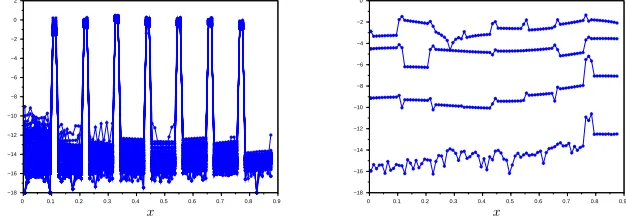
Fig. 1. Illustration of the residual when RAS is used as a nonlinear solver (left) or as a

preconditioner for Newton’s method (right).

because it is this equation that holds at the fixed point of iteration (2.5). We call this

method one-level RASPEN. We show in Figure 1 as an example the residual of the

nonlinear RAS iterations and using RASPEN as a preconditioner for Newton when

solving the Forchheimer equation with eight subdomains from the numerical section.

We observe that the residual of the nonlinear RAS method is concentrated at the

interfaces, since it must be zero inside the subdomains by construction. Thus, when

Newton’s method is used to solve (2.6), it only needs to concentrate on reducing the

residual on a small number of interface variables. This explains the fast convergence

of RASPEN shown on the right of Figure 1, despite the slow convergence of the

underlying RAS iteration.

Suppose we also want to include a coarse grid correction step in the Schwarz

iteration (2.2), or equivalently in (2.5). Since the problem is nonlinear, we need to

use the FAS from multigrid to do so (see, for example, [3, 27]): given an approximate

solution

u

n−1

_{, we compute the correction}

_c

_{by solving the nonlinear coarse problem}

(2.7)

L

c

₍

_R

0

u

n−1

+

c

) =

L

c

(

R

0

u

n−1

) + ˜

R

0

(

f

− L

(

u

n−1

))

,

where

L

c

_{is a coarse approximation of the nonlinear problem (2.1) and}

_R

0

is a

restric-tion operator. This correcrestric-tion

c

:=

C

0

(

u

n−1

) is then added to the iterate to get the

new corrected value

(2.8)

u

nnew−1

=

u

n−1

+

P

0

C

0

(

u

n−1

)

,

where

P

0

is a suitable prolongation operator. Introducing this new approximation

from (2.8) at step

n

−

1 into the subdomain iteration formula (2.5), we obtain the

method with integrated coarse correction

(2.9)

u

n

=

I

X

i=1

e

P

i

G

i

(

u

n−1

+

P

0

C

0

(

u

n−1

)) =:

G

2

(

u

n−1

)

.

This stationary fixed point iteration can also be accelerated using Newton’s method:

we can use Newton to solve the nonlinear equation

(2.10)

F

˜

2

(

u

) :=

G

2

(

u

)

−

u

=

I

X

i=1

e

P

i

G

i

(

u

+

P

0

C

0

(

u

))

−

u

= 0

.

[image:4.612.93.406.112.224.2]

We call this method two-level FAS-RASPEN.

We have written the coarse step as a correction, but not the subdomain steps.

This, however, can also be done, by simply rewriting (2.5) to add and subtract the

previous iterate,

(2.11)

u

n

=

u

n−1

+

I

X

i=1

e

P

i

(

G

i

(

u

n−1

)

−

R

i

u

n−1

)

|

{z

}

=:Ci(un−1)

=

u

n−1

+

I

X

i=1

e

P

i

C

i

(

u

n−1

)

,

where we have assumed that

P

i

P

˜

i

R

i

=

I

V

, the identity on the vector space; see

Assumption 1 in the next section. Together with the coarse grid correction (2.8), this

iteration then becomes

(2.12)

u

n

=

u

n−1

+

P

0

C

0

(

u

n−1

) +

I

X

i=1

e

P

i

C

i

(

u

n−1

+

P

0

C

0

(

u

n−1

))

,

which can be accelerated by solving with Newton the equation

(2.13)

F

˜

2

(

u

) :=

P

0

C

0

(

u

) +

I

X

i=1

e

P

i

C

i

(

u

+

P

0

C

0

(

u

)) = 0

.

This is equivalent to ˜

F

2

(

u

) = 0 from (2.10), only written in correction form.

3. Definition of RASPEN and comparison with ASPIN.

We now define

formally the one- and two-level versions of the RASPEN method and compare them

with the respective ASPIN methods. We consider a nonlinear function

F

:

V

→

V

0

,

where

V

is a Hilbert space, and the nonlinear problem of finding

u

∈

V

such that

(3.1)

F

(

u

) = 0

.

Let

V

i

, i

= 1

, . . . , I

, be Hilbert spaces, which would generally be subspaces of

V

.

We consider for all

i

= 1

, . . . , I

the linear restriction and prolongation operators

R

i

:

V

→

V

i

,

P

i

:

V

i

→

V

, as well as the “restricted” prolongation

P

e

i

:

V

i

→

V

.

Assumption

1. We assume that

R

i

and

P

i

satisfy for

i

= 1

, . . . , I

R

i

P

i

=

I

Vi

,

the identity on

V

i

,

and that

R

i

and

P

e

i

satisfy

PIi=1PeiRi=IV

.

These are all the assumptions we need in what follows, but it is helpful to think

of the restriction operators

R

i

as classical selection matrices which pick unknowns

corresponding to the subdomains Ω

i

, of the prolongations

P

i

as

R

Ti

, and of the

P

e

i

as

extensions based on a nonoverlapping decomposition.

3.1. One- and two-level RASPEN.

We can now formulate precisely the

RASPEN method from the previous section: we define the local inverse

G

i

:

V

→

V

i

to be solutions of

(3.2)

R

i

F

(

P

i

G

i

(

u

) + (

I

−

P

i

R

i

)

u

) = 0

.

In the usual PDE framework, this corresponds to solving locally on the subdomain

i

the PDE problem on

V

i

with Dirichlet boundary condition given by

u

outside of the

subdomain

i

; see (2.4). Then, one-level RASPEN solves the nonlinear equation

(3.3)

F

˜

1

(

u

) =

I

X

i=1

e

P

i

G

i

(

u

)

−

u

= 0

using Newton’s method; see (2.6). The preconditioned nonlinear function (3.3)

cor-responds to the fixed point iteration

(3.4)

u

n

=

I

X

i=1

e

P

i

G

i

(

u

n−1

);

see (2.5). Equivalently, the RASPEN equation (3.3) can be written in correction form

as

(3.5)

F

˜

1

(

u

) =

I

X

i=1

e

P

i

(

G

i

(

u

)

−

R

i

u

) =:

I

X

i=1

e

P

i

C

i

(

u

)

,

where we define the corrections

C

i

(

u

) :=

G

i

(

u

)

−

R

i

u

. This way, the subdomain solves

(3.2) can be written in terms of

C

i

(

u

) as

(3.6)

R

i

F

(

u

+

P

i

C

i

(

u

)) = 0

.

In the special case where

F

(

u

) =

Au

−

b

is affine, (3.6) reduces to

R

i

A

(

u

+

P

i

C

i

(

u

))

−

R

i

b

= 0 =

⇒

C

i

(

u

) =

A

i−1

R

i

(

b

−

Au

)

,

where

A

i

=

R

i

AP

i

is the subdomain matrix. This implies

˜

F

1

(

u

) =

I

X

i=1

e

P

i

A

−i 1

R

i

(

b

−

Au

)

,

and we immediately see that the Jacobian is the matrix

A

preconditioned by the RAS

preconditioner

P

I

i=1

P

e

i

A

−i1

R

i

. Thus, if a Krylov method is used to solve the outer

system, our method is equivalent to the Krylov-accelerated one-level RAS method in

the linear case.

To define the two-level variant, we introduce a coarse space

V

0

and the linear

re-striction and prolongation operators

R

0

:

V

→

V

0

,

P

0

:

V

0

→

V

. Let

F

0

:

V

0

→

V

00

be

the coarse nonlinear function, which could be defined by using a coarse discretization

of the underlying problem, or using a Galerkin approach we use here, namely,

(3.7)

F

0

(

u

0

) =

R

e

0

F

(

P

0

(

u

0

))

.

Here,

R

e

0

:

V

0

→

V

00

is a projection operator that plays the same role as

R

0

, but in

the residual space. In two-level FAS-RASPEN, we use the well-established nonlinear

coarse correction

C

0

(

u

) from the FAS already shown in (2.7), which in the rigorous

context of this section is defined by

(3.8)

F

0

(

C

0

(

u

) +

R

0

u

) =

F

0

(

R

0

u

)

−

R

e

0

F

(

u

)

.

This coarse correction is used in a multiplicative fashion in RASPEN, i.e., we solve

with Newton the preconditioned nonlinear system

(3.9)

F

e

2

(

u

) =

P

0

C

0

(

u

) +

n

X

i=1

e

P

i

C

i

(

u

+

P

0

C

0

(

u

)) = 0

.

This corresponds to the nonlinear two-level fixed point iteration

u

n+1

=

u

n

+

P

0

C

0

(

u

n

) +

n

X

i=1

e

P

i

C

i

(

u

n

+

P

0

C

0

(

u

n

))

0 2 4 6 8 10 12 14 16 18 20 22 24 0 −10 −8 −6 −4 −2 2 4 6 −9 −7 −5 −3 −1 1 3 5 Iteration n Newton One Level AS Two level AS One Level ASPIN Two level ASPIN

0 2 4 6 8 10 12 14 16 18 20 22 24

0 −10 −8 −6 −4 −2 2 4 6 −9 −7 −5 −3 −1 1 3 5 Iteration n Newton One Level RAS Two level RAS One Level RASPEN Two level FA−RASPEN

0 20 40 60 80 100 120 140 160 180

0 −10 −8 −6 −4 −2 2 4 6 −9 −7 −5 −3 −1 1 3 5

Linear subdomain solves

Newton One Level AS Two level AS One Level ASPIN Two level ASPIN

0 20 40 60 80 100 120 140 160 180 0 −10 −8 −6 −4 −2 2 4 6 −9 −7 −5 −3 −1 1 3 5

Linear subdomain solves

Newton One Level RAS Two level RAS One Level RASPEN Two level FA−RASPEN

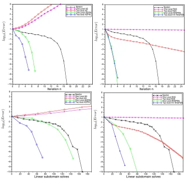
Fig. 2. Error as function of nonlinear iteration numbers in the top row and as number of

subdomain solves in the bottom row for ASPIN (left) and RASPEN (right).

with

C

0

(

u

n

) defined in (3.8) and

C

i

(

u

n

) defined in (3.6). This iteration is convergent,

as we can see in Figure 2 in the right column. In the special case of an affine residual

function

F

(

u

) =

Au

−

b

, a simple calculation shows that

e

F

2

(

u

) =

P

0

A

−01

R

e

0

+

I

X

i=1

e

P

i

A

−i1

R

i

(

I

V

−

AP

0

A

−01

R

e

0

)

!

(

b

−

Au

)

,

where we assumed that the coarse function

F

0

=

A

0

u

0

−

b

0

is also linear. Thus, in the

linear case, two-level RASPEN corresponds to preconditioning by a two-level RAS

preconditioner, where the coarse grid correction is applied multiplicatively.

3.2. Comparison of one-level variants.

In order to compare RASPEN with

the existing ASPIN method, we recall the precise definition of one-level ASPIN from

[8], which gives a different reformulation

F

1

(

u

) = 0 of the original equation (3.1) to

be solved. In ASPIN, one also defines for

u

∈

V

and for all

i

= 1

, . . . , I

the corrections

as in (3.6), i.e., we define

C

i

(

u

)

∈

V

i

such that

R

i

F

(

u

+

P

i

C

i

(

u

)) = 0

,

[image:7.612.70.439.90.446.2]

where

P

i

C

i

(

u

) are called

T

i

in [8]. Then, the one-level ASPIN preconditioned function

is defined by

(3.10)

F

1

(

u

) =

I

X

i=1

P

i

C

i

(

u

)

,

and the preconditioned system

F

1

(

u

) = 0 is solved using a Newton algorithm with an

inexact Jacobian; see section 3.4. The ASPIN preconditioner also has a corresponding

fixed point iteration: adding and subtracting

P

i

R

i

u

in the definition (3.6) of the

corrections

C

i

, we obtain

R

i

F

(

u

+

P

i

C

i

(

u

)) =

R

i

F

(

P

i

(

R

i

u

+

C

i

(

u

)) +

u

−

P

i

R

i

u

) = 0

,

which implies, by comparing with (3.2) and assuming existence and uniqueness of the

solution to the local problems, that

G

i

(

u

) =

R

i

u

+

C

i

(

u

)

.

We therefore obtain for one-level ASPIN

(3.11)

F

1

(

u

) =

I

X

i=1

P

i

C

i

(

u

) =

I

X

i=1

P

i

G

i

(

u

)

−

I

X

i=1

P

i

R

i

u,

which corresponds to the nonlinear fixed point iteration

(3.12)

u

n

=

u

n−1

+

I

X

i=1

P

i

C

i

(

u

n−1

) =

u

n−1

−

I

X

i=1

P

i

R

i

u

n−1

+

I

X

i=1

P

i

G

i

(

u

n−1

)

.

This iteration is not convergent in the overlap, already in the linear case (see [14, 20]),

and needs a relaxation parameter to yield convergence; see, for example, [12] for

the nonlinear case. This can be seen directly from (3.12): if an overlapping region

belongs to

K

subdomains, then the current iterate

u

n

_{is subtracted}

_K

_{times there,}

and then the sum of the

K

respective subdomain solutions is added to the result.

This redundancy is avoided in our formulation (3.4). The only interest in using an

additive correction in the overlap is that in the linear case, the preconditioner remains

symmetric for a symmetric problem.

We show in Figure 2 a numerical comparison of the two methods, together with

Newton’s method applied directly to the nonlinear problem, for the first example of the

Forchheimer equation from section 4.1 on a domain of unit size with eight subdomains,

overlap 3

h

, with

h

= 1

/

100. In these comparisons, we use ASPIN first as a fixed-point

iterative solver (labeled AS for additive Schwarz) and then as a preconditioner. We do

the same for our new nonlinear iterative method, which in the figures is labeled RAS.

We see from this numerical experiment that ASPIN as an iterative solver (AS) does

not converge, whereas RASPEN used as an iterative solver (RAS) does, both with

and without coarse grid. Also note that two-level RAS is faster than Newton directly

applied to the nonlinear problem for small iteration counts, before the superlinear

convergence of Newton kicks in. The fact that RASPEN is based on a convergent

iteration, but not ASPIN, has an important influence also on the Newton iterations

when the methods are used as preconditioners: the ASPIN preconditioner requires

more Newton iterations to converge than RASPEN does. At first sight, it might

be surprising that in RASPEN, the number of Newton iterations with and without

coarse grid is almost the same, while ASPIN needs more iterations without coarse

grid. In contrast to the linear case with Krylov acceleration, it is not the number

of Newton iterations that depends on the number of subdomains, but the number of

linear inner iterations within Newton, which grows when no coarse grid is present.

We show this in the second row of Figure 2, where now the error is plotted as a

function of the maximum number of linear subdomain solves used in each Newton

step; see subsection 4.1.1. With this more realistic measure of work, we see that both

RASPEN and ASPIN converge substantially better with a coarse grid, but RASPEN

needs many fewer subdomain solves than ASPIN does.

3.3. Comparison of two-level variants.

We now compare two-level

RASPEN with the two-level ASPIN method of [32]. Recall that the two-level

FAS-RASPEN consists of applying Newton’s method to (3.9),

e

F

2

(

u

) =

P

0

C

0

(

u

) +

n

X

i=1

e

P

i

C

i

(

u

+

P

0

C

0

(

u

)) = 0

,

where the corrections

C

0

(

u

) and

C

i

(

u

) are defined in (3.8) and (3.6), respectively.

Unlike FAS-RASPEN, two-level ASPIN requires the solution

u

∗₀

∈

V

0

to the coarse

problem, i.e.,

F

0

(

u

∗0

) = 0, which can be computed in a preprocessing step.

In two-level ASPIN, the coarse correction

C

0A

:

V

→

V

0

is defined by

(3.13)

F

0

(

C

0A

(

u

) +

u

∗0

) =

−

R

e

0

F

(

u

)

,

and the associated two-level ASPIN function uses the coarse correction in an additive

fashion, i.e., Newton’s method is used to solve

(3.14)

F

2

(

u

) =

P

0

C

0A

(

u

) +

I

X

i=1

P

i

C

i

(

u

) = 0

with

C

A

0

(

u

n

) defined in (3.13) and

C

i

(

u

n

) defined in (3.6). This is in contrast to

two-level FAS-RASPEN, where the coarse correction

C

0

(

u

) is computed from the

well-established FAS and is applied multiplicatively in (3.9). The fixed point iteration

corresponding to (3.14) is

u

n+1

=

u

n

+

P

0

C

0A

(

u

n

_{) +}

I

X

i=1

P

i

C

i

(

u

n

)

.

Just like its one-level counterpart, two-level ASPIN is not convergent as a fixed-point

iteration without a relaxation parameter; see Figure 2 in the left column. Moreover,

because the coarse correction is applied additively, the overlap between the coarse

space and subdomains leads to slower convergence in the Newton solver, which does

not happen with FAS-RASPEN.

3.4. Computation of Jacobian matrices.

When solving (3.5), (3.9), (3.11),

and (3.14) using Newton’s method, one needs to repeatedly solve linear systems

in-volving Jacobians of the above functions. If one uses a Krylov method such as GMRES

to solve these linear systems, like we do in this paper, then it suffices to have a

pro-cedure for multiplying the Jacobian with an arbitrary vector. In this section, we

derive the Jacobian matrices for both one-level and two-level RASPEN in detail. We

compare these expressions with ASPIN, which approximates the exact Jacobian with

an inexact one in an attempt to reduce the computational cost, even though this can

potentially slow down the convergence of Newton’s method. Finally, we show that

this approximation is not necessary in RASPEN: in fact, all the components involved

in building the exact Jacobian have already been computed elsewhere in the

algo-rithm, so there is little additional cost in using the exact Jacobian compared with the

approximate one.

3.4.1. Computation of the one-level Jacobian matrices.

We now show

how to compute the Jacobian matrices of ASPIN and RASPEN. To simplify notation,

we define

(3.15)

u

(i)

:=

P

i

G

i

(

u

) + (

I

−

P

i

R

i

)

u

and

J

(

v

) :=

dF

du

(

v

)

.

By differentiating (3.2), we obtain

(3.16)

dG

i

du

(

u

) =

−

(

R

i

J

(

u

(i)

₎

_P

i

)

−1

R

i

J

(

u

(i)

) +

R

i

.

We deduce for the Jacobian of RASPEN from (3.3)

(3.17)

d

˜

F

1

du

(

u

) =

I

X

i=1

e

P

i

dG

i

du

(

u

)

−

I

=

−

I

X

i=1

e

P

i

(

R

i

J

(

u

(i)

)

P

i

)

−1

R

i

J

(

u

(i)

)

,

since the identity cancels. Similarly, we obtain for the Jacobian of ASPEN (additive

Schwarz preconditioned exact Newton) in (3.11)

(3.18)

d

F

1

du

(

u

) =

I

X

i=1

P

i

dG

i

du

(

u

)

−

I

X

i=1

P

i

R

i

=

−

I

X

i=1

P

i

(

R

i

J

(

u

(i)

)

P

i

)

−1

R

i

J

(

u

(i)

)

,

since now the terms

P

I

i=1

P

i

R

i

cancel. In ASPIN, this exact Jacobian is replaced by

the inexact Jacobian

d

F

1

du

inexact

(

u

) =

−

I

X

i=1

P

i

(

R

i

J

(

u

)

P

i

)

−1

R

i

!

J

(

u

)

.

We see that this is equivalent to preconditioning the Jacobian

J

(

u

) of

F

(

u

) by the

additive Schwarz preconditioner, up to the minus sign. This can be convenient if one

already has a code for this, as it was noted in [8]. The exact Jacobian is, however,

also easily accessible, since the Newton solver for the nonlinear subdomain system

R

i

F

(

P

i

G

i

(

u

) + (

I

−

P

i

R

i

)

u

) = 0 already computes and factorizes the local Jacobian

matrix

R

i

J

(

u

(i)

)

P

i

. Therefore, the only missing ingredient for computing the exact

Jacobian of

F

1

is the matrices

R

i

J

(

u

(i)

), which only differ from

R

i

J

(

u

(i)

)

P

i

by a few

additional columns, corresponding in the usual PDEs framework to the derivative

with respect to the Dirichlet boundary conditions. In contrast, the computation of

the inexact ASPIN Jacobian requires one to recompute the entire Jacobian of

F

(

u

)

after the subdomain nonlinear solves.

3.4.2. Computation of the two-level Jacobian matrices.

We now compare

the Jacobians for the two-level variants. For RASPEN, we need to differentiate ˜

F

2

with respect to

u

, where ˜

F

2

is defined in (3.9):

e

F

2

(

u

) =

P

0

C

0

(

u

) +

n

X

i=1

e

P

i

C

i

(

u

+

P

0

C

0

(

u

))

.

To do so, we need

dC0

du

and

dCi

du

for

i

= 1

, . . . , I

. The former can be obtained by

differentiating (3.8):

F

₀0

(

R

0

u

+

C

0

(

u

))

R

0

+

dC

0

du

=

F

₀0

(

R

0

u

)

R

0

−

R

e

0

F

0

(

u

)

.

Thus, we have

(3.19)

dC

0

du

=

−

R

0

+ ˆ

J

−1

0

(

J

0

R

0

−

R

e

0

J

(

u

))

,

where

J

0

=

F

00

(

R

0

u

) and ˆ

J

0

=

F

00

(

R

0

u

+

C

0

(

u

)). Note that the two Jacobian matrices

are evaluated at different arguments, so no cancellation is possible in (3.19) except in

special cases (e.g., if

F

0

is an affine function). Nonetheless, they are readily available:

ˆ

J

0

is simply the Jacobian for the nonlinear coarse solve, so it would have already been

calculated and factorized by Newton’s method.

J

0

would also have been calculated

during the coarse Newton iteration if

R

0

u

is used as the initial guess.

We also need

dCi

du

from the subdomain solves. From the relation

G

i

(

u

) =

R

i

u

+

C

i

(

u

)

,

we deduce immediately from (3.16) that

(3.20)

dC

i

du

=

dG

i

du

−

R

i

=

−

(

R

i

J

(

u

(i)

₎

_P

i

)

−1

R

i

J

(

u

(i)

)

,

where

u

(i)

₌

_u

₊

_P

i

C

i

(

u

)

.

Thus, the Jacobian for the two-level RASPEN function is

(3.21)

d

F

e

2

du

=

P

0

dC

0

du

−

X

i

˜

P

i

(

R

i

J

(

v

(i)

)

P

i

)

−1

R

i

J

(

v

(i)

)

I

+

P

0

dC

0

du

,

where

dC0

du

is given by (3.19) and

v

(i)

₌

_u

₊

_P

0

C

0

(

u

) +

P

i

C

i

(

u

+

P

0

C

0

(

u

))

.

For completeness, we compute the Jacobian for two-level ASPIN. First, we obtain

dCA

0

du

by differentiating (3.13), which gives

(3.22)

dC

A

0

du

=

−

ˆ

J

₀−1

R

e

0

J

(

u

)

,

where ˆ

J

0

=

F

00

(

C

0A

(

u

) +

u

∗0

)

.

In addition, two-level ASPIN uses as approximation for

(3.20)

(3.23)

dC

i

du

≈ −

(

R

i

J

(

u

)

P

i

)

−1

_R

i

J

(

u

)

.

Thus, the inexact Jacobian for the two-level ASPIN function is

(3.24)

d

F

2

du

≈ −

P

0

ˆ

J

₀−1

R

e

0

J

(

u

)

−

X

i

P

i

(

R

i

J

(

u

)

P

i

)

−1

R

i

J

(

u

)

.

Comparing (3.21) with (3.24), we see two major differences.

First,

dC

0

/du

only

simplifies to

−

R

e

0

J

(

u

) if

J

0

= ˆ

J

0

, i.e., if

F

0

is affine. Second, (3.21) resembles a

two-stage multiplicative preconditioner, whereas (3.24) is of the additive type. This is due

to the fact that the coarse correction in two-level RASPEN is applied multiplicatively,

whereas two-level ASPIN uses an additive correction.

4. Numerical experiments.

In this section, we compare the new nonlinear

preconditioner RASPEN to ASPIN for the Forchheimer model, which generalizes the

linear Darcy model in porous media flow [18, 36, 10], and for a 2D nonlinear diffusion

problem that appears in [1].

4.1. Forchheimer model and discretization.

Let us consider the

Forch-heimer parameter

β >

0, the permeability

λ

∈

L

∞

(Ω) such that 0

< λ

min

≤

λ

(

x

)

≤

λ

max

for all

x

∈

Ω, and the function

q

(

g

) = sgn(

g

)

−1+

√

1+4β|g|

2β

. The Forchheimer

model on the interval Ω = (0

, L

) is defined by the equation

(4.1)







(

q

(

−

λ

(

x

)

u

(

x

)

0

₎₎

0

₌

_f

₍

_x

₎

_{in Ω}

_,

u

(0) =

u

D

0

,

u

(

L

) =

u

D

L

.

Note that at the limit when

β

→

0

+

_{, we recover the linear Darcy equation. We}

consider a 1D mesh defined by the

M

+ 1 points

0 =

x

1

2

<

· · ·

< x

K+12

<

· · ·

< x

M+12

=

L.

The cells are defined by

K

= (

x

_K−1

2

, x

K+12

) for

K

∈ M

=

{

1

, . . . , M

}

and their

center by

x

K

=

x_K−1

2

+x

K+ 1₂

2

. The Forchheimer model (4.1) is discretized using a

two point flux approximation (TPFA) finite volume scheme. We define the TPFA

transmissibilities by



















T

_K+1 2

=

1

|x_{K+ 1}

2−

xK|

λK

+

|xK+1−xK+ 1₂|

λK+1

for

K

= 1

, . . . , M

−

1

,

T

1 2

=

λ

1

|

x

1

−

x

1

2

|

,

T

_M+1 2

=

λ

M

|

x

_M+1

2

−

x

M

|

,

with

λ

K

=

_|x 1 K+ 1₂−xK−1

2 |

R

xK+ 1₂

x_K−1

2

λ

(

x

)

dx

. Then, the

M

cell unknowns

u

K

,

K

∈ M

,

are the solution of the set of

M

conservation equations











q

(

T

K+1

2

(

u

K

−

u

K+1

)) +

q

(

T

K− 1

2

(

u

K

−

u

K−1

)) =

f

K

, K

= 2

, . . . , M

−

1

,

q

(

T

3

2

(

u

1

−

u

2

)) +

q

(

T

1

2

(

u

1

−

u

D

0

)) =

f

1

,

q

(

T

_M+1

2

(

u

M

−

u

D

L

)) +

q

(

T

M−1

2

(

u

M

−

u

M−1

)) =

f

M

,

with

f

K

=

R

xK+ 1₂

x_K−1

2

f

(

x

)

dx

. In the following numerical tests we will consider a uniform

mesh of cell size denoted by

h

=

L

M

.

4.1.1. One-level variants.

We start from a nonoverlapping decomposition of

the set of cells

f

Mi

, i

= 1

, . . . , I,

such that

M

=

S

i=1,...,I

M

f

i

and

M

f

i

∩

M

f

j

=

∅

for all

i

6

=

j

.

The overlapping decomposition

M

i

, i

= 1

, . . . , I

, of the set of cells is obtained

by adding

k

layers of cells to each

Mi

f

to generate overlap with the two neighboring

subdomains

Mi

f

−1

(if

i >

1) and

Mi

f

+1

(if

i < I

) in the simple case of our 1D domain.

In the ASPIN framework, we set

V

=

R

#M

, and

V

i

=

R

#Mi

_,

_i

_{= 1}

_{, . . . , I}

_{. The}

restriction operators are then defined by

(

R

i

v

)

K

=

v

K

for

K

∈ Mi

,

0 0.2 0.4 0.6 0.8 1 1.2 1.4 1.6 0

1

0.2 0.4 0.6 0.8

0.1 0.3 0.5 0.7 0.9 1.1

permeability

0 0.2 0.4 0.6 0.8 1 1.2 1.4 1.6

0

−60 −40 −20 20 40 60

−50 −30 −10 10 30 50

right hand side

0 0.2 0.4 0.6 0.8 1 1.2 1.4 1.6 0

−2

−3 −1 1

−2.8 −2.6 −2.4 −2.2 −1.8 −1.6 −1.4 −1.2 −0.8 −0.6 −0.4 −0.2 0.2 0.4 0.6

0.8 Initial guess Exact solution

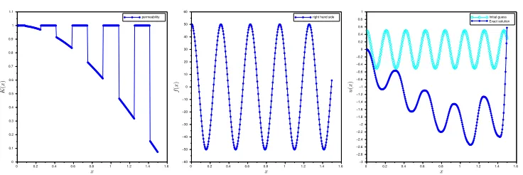
Fig. 3. Permeability field (left), source term (middle), initial guess and solution (right).

and the prolongation operators are

(

P

i

v

i

)

K

=

v

K

for

K

∈ Mi

,

(

P

i

v

i

)

K

= 0 for

K

6∈ Mi

,

and

(

(

P

e

i

v

i

)

K

=

v

K

for

K

∈

Mi

f

,

(

P

e

i

v

i

)

K

= 0 for

K

6∈

Mi

f

.

The coarse grid is obtained by the agglomeration of the cells in each

Mi

f

defining a

coarse mesh of (0

, L

).

Finally, we set

V

0

=

R

I

. In the finite volume framework, we define for all

v

∈

V

(

R

0

v

)

i

=

1

#

M

f

i

X

K∈Mfi

v

K

for all

i

= 1

, . . . , I,

(

R

e

0

v

)

i

=

X

K∈Mfi

v

K

for all

i

= 1

, . . . , I.

In our case of a uniform mesh,

R

0

corresponds to the mean value in the coarse cell

i

for cellwise constant functions on

M

, whereas

R

e

0

corresponds to the aggregate flux

over the coarse cell

M

f

i

.

For

v

0

∈

V

0

, its prolongation

v

=

P

0

v

0

∈

V

is obtained by the piecewise linear

interpolation

ϕ

(

x

) on (0

, x

1

), (

x

1

, x

2

)

, . . . ,

(

x

I

, L

), where the

x

i

are the centers of the

coarse cells, and

ϕ

(

x

i

) = (

v

0

)

i

,

i

= 1

, . . . , I

,

ϕ

(0) = 0,

ϕ

(

L

) = 0. Then,

v

=

P

0

v

0

is

defined by

v

K

=

ϕ

(

x

K

) for all

K

∈ M

. The coarse grid operator

F

0

is defined by

F

0

(

v

0

) =

R

e

0

F

(

P

0

v

0

) for all

v

0

∈

V

0

.

We use for the numerical tests the domain Ω = (0

,

3

/

2) with the boundary

con-ditions

u

(0) = 0 and

u

(3

/

2) = 1, and different values of

β

. As a first challenging test,

we choose the highly variable permeability field

λ

and the oscillating right-hand side

shown in Figure 3. We measure the relative

l

1

_{norms of the error obtained at each}

Newton iteration as a function of the parallel linear solves

LS

n

needed in the

subdo-mains per Newton iteration, which is a realistic measure for the cost of the method.

Each Newton iteration requires two major steps:

1. The evaluation of the fixed point function

F

, which means solving a nonlinear

problem in each subdomain. This is done using Newton in an inner iteration

on each subdomain and thus requires at each inner iteration a linear

subdo-main solve performed in parallel by all subdosubdo-mains (we have used a sparse

direct solver for the linear subdomain solves in our experiments, but one can

also use an iterative method if good preconditioners are available). We denote

[image:13.612.76.444.89.212.2]

the maximum number of inner iterations needed by the subdomains at the

outer iteration

j

by

ls

in

j

, and it is the maximum which is relevant, because

if other subdomains finish earlier, they still have to wait for the last one to

finish.

2. The Jacobian matrix needs to be inverted, which we do by GMRES, and each

GMRES iteration will also need a linear subdomain solve per subdomain. We

denote the number of linear solves needed by GMRES at the outer Newton

iteration step

j

by

ls

G_j

.

Hence, the number of linear subdomain solves for the outer Newton iteration

j

to

complete is

ls

in_j

+

ls

G_j

, and the total number of linear subdomain solves after

n

outer

Newton iterations is

LS

n

:=

P

n

j=1

ls

in

j

+

ls

G j

. In all the numerical tests, we stop

the linear GMRES iterations when the relative residual falls below 10

−8

, and the

tolerances for the inner and outer Newton iterations are also set to 10

−8

. Adaptive

tolerances could certainly lead to more savings [15, 16], but our purpose here is to

compare the nonlinear preconditioners in a fixed setting. The initial guess we use in

all our experiments is shown in Figure 3 on the right, together with the solution.

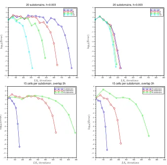
We show in Figure 4 how the convergence depends on the overlap and the number

of subdomains for one-level ASPIN and RASPEN with Forchheimer model parameter

β

= 1. In the top row on the left of Figure 4, we see that for ASPIN the number

of linear iterations increases much more rapidly when decreasing the overlap than

for RASPEN on the right for a fixed mesh size

h

= 0

.

003 and number of subdomains

equals 20. In the bottom row of Figure 4, we see that the convergence of both one-level

ASPIN and RASPEN depends on the number of subdomains, but RASPEN seems to

be less sensitive than ASPIN.

4.1.2. Two-level variants.

In Figure 5, we show the dependence of two-level

ASPIN and two-level FAS-RASPEN on a decreasing size of the overlap, as we did

for the one-level variants in the top row of Figure 4. We see that the addition of the

coarse level improves the performance for RASPEN when the overlap is large and in

all cases for ASPIN.

In Figure 6, we present a study of the influence of the number of subdomains

on the convergence for two-level ASPIN and two-level FAS-RASPEN with different

values of the Forchheimer parameter

β

= 1

,

0

.

1

,

0

.

01 which governs the nonlinearity

of the model (the model becomes linear for

β

= 0). An interesting observation is

that for

β

= 1, the convergence of both two-level ASPIN and two-level FAS-RASPEN

depends on the number of subdomains in an irregular fashion: increasing the number

of subdomains sometimes increases iteration counts, and then decreases them again.

We will study this effect further below, but note already from Figure 6 that this

dependence disappears for two-level FAS-RAPSEN as the nonlinearity diminishes

(i.e., as

β

decreases) and is weakened for two-level ASPIN.

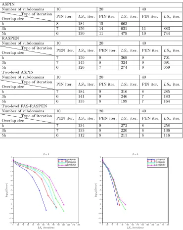
We finally show in Table 1 the number of outer Newton iterations (PIN iter

for ASPIN and PEN iter for RASPEN) and the total number of linear iterations

(

LS

n

iter) for various numbers of subdomains and various overlap sizes obtained with

ASPIN, RASPEN, two-level ASPIN, and two-level FAS-RASPEN. We see that the

coarse grid considerably improves the convergence of both RASPEN and ASPIN.

Also, in all cases, RASPEN needs substantially fewer linear iterations than ASPIN.

We now return to the irregular number of iterations observed in Figure 6 for

the Forchheimer parameter

β

= 1, i.e., when the nonlinearity is strong. We claim

that this irregular dependence is due to strong variations in the initial guesses used

0 100 200 300 400 500 600 700 800 900 0

−10 −8 −6 −4 −2 2 4

−9 −7 −5 −3 −1 1 3

h 3h 9h 15h 20 subdomains, h=0.003

0 100 200 300 400 500 600 700 800 900

0

−10 −8 −6 −4 −2 2 4

−9 −7 −5 −3 −1 1 3

h 3h 9h 15h 20 subdomains, h=0.003

0 100 200 300 400 500 600 700 800 900 0

−10

−12 −8 −6 −4 −2 2 4

−11 −9 −7 −5 −3 −1 1 3

10 subdomains 20 subdomains 40 subdomains

15 cells per subdomain, overlap 3h

0 100 200 300 400 500 600 700 800 900 0

−10

−12 −8 −6 −4 −2 2 4

−11 −9 −7 −5 −3 −1 1 3

10 subdomains 20 subdomains 40 subdomains 15 cells per subdomain, overlap 3h

Fig. 4.Error obtained with one-level ASPIN (left) and one-level RASPEN (right): in the top

row obtained with20subdomains,h= 0.003, and decreasing size of overlap15h,9h,3h,h; in the

bottom row obtained with different numbers of subdomains10,20, and40, overlap3h, and a fixed

number of cells per subdomain. The Forchheimer problem is defined by the permeability, source

term, solution, and initial guess of Figure3.

by RASPEN and ASPIN at subdomain interfaces, which is in turn caused by the

highly variable contrast and oscillating source term we used, leading to an oscillatory

solution; see Figure 3. In other words, we expect the irregularity to disappear when

the solution is nonoscillatory. To test this, we now present numerical results with the

less variable permeability function

λ

(

x

) = cos(

x

) and source term

f

(

x

) = cos(

x

) as

well, which leads to a smooth solution. Starting with a zero initial guess, we show in

Figure 7 the results obtained for Forchheimer parameter

β

= 1, corresponding to the

first row of Figure 6.

We clearly see that the irregular behavior has now disappeared for both

two-level ASPIN and RASPEN, but two-two-level ASPIN still shows some dependence of the

iteration numbers as the number of subdomains increases. We show in Table 2 the

complete results for this smoother example, and we see that the irregular convergence

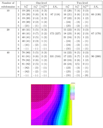
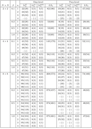
behavior of the two-level methods is no longer present. We finally give in Table 3 a

detailed account of the linear subdomain solves needed for each outer Newton iteration

n

for the case of an overlap of 3

h

. There, we use the format

it

RASPEN

(

it

ASPIN

), where

[image:15.612.89.428.89.424.2]

0 100 200 300 400 500 600 700 800 900 0

−10 −8 −6 −4 −2 2 4

−9 −7 −5 −3 −1 1 3

h 3h 9h 15h 20 subdomains, h=0.003

0 100 200 300 400 500 600 700 800 900 0

−10 −8 −6 −4 −2 2 4

−9 −7 −5 −3 −1 1 3

h 3h 9h 15h

20 subdomains, h=0.003

Fig. 5.Error obtained with two-level ASPIN (left) and two-level FAS RASPEN (right) obtained

with20subdomains,h= 0.003, and decreasing overlap 15h,9h,3h,h. The Forchheimer problem

is defined by the permeability, source term, solution, and initial guess of Figure3.

it

RASPEN

is the iteration count for RASPEN and

it

ASPIN

is the iteration count for

ASPIN. We show in the first column the linear subdomain solves

ls

G

n

required for the

inversion of the Jacobian matrix using GMRES (see item 2 in subsection 4.1.1) and

in the next column the maximum number of iterations

ls

in

n

needed to evaluate the

nonlinear fixed point function

F

(see item 1 in subsection 4.1.1). In the next column,

we show for completeness also the smallest number of inner iterations

ls

min

n

any of the

subdomains needed, to illustrate how balanced the work is in this example. The last

column then contains the total number of linear iterations

LS

n

; see subsection 4.1.1.

These results show that the main gain of RASPEN is a reduced number of Newton

iterations, i.e., it is a better nonlinear preconditioner than ASPIN, and also a reduced

number of inner iterations for the nonlinear subdomain solves, i.e., the preconditioner

is less expensive. This leads to the substantial savings observed in the last columns

and in Table 2.

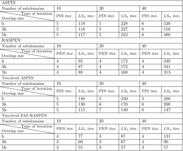
4.2. A nonlinear Poisson problem.

We now test the nonlinear

precondition-ers on the 2D nonlinear diffusion problem (see [1])

(4.2)











−∇ ·

((1 +

u

2

)

∇

u

)

=

f,

Ω = [0

,

1]

2

,

u

=

1

,

x

= 1

,

∂u

∂

n

=

0

otherwise.

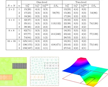
The isovalues of the exact solution are shown in Figure 8. To calculate this solution,

we use a discretization with P1 finite elements on a uniform triangular mesh. All

calculations have been performed using FreeFEM++, a C++ based domain-specific

language for the numerical solution of PDEs using finite element methods [26]. We

consider a decomposition of the domain into

N

×

N

subdomains with an overlap of

one mesh size

h

, and we keep the number of degrees of freedom per subdomain fixed

in our experiments. We show in Table 4 a detailed account of the number of linear

subdomain solves needed for RASPEN and ASPIN at each outer Newton iteration

n

, using the same notation as in Table 3 (Newton converged in three iterations for

all examples to a tolerance of 10

−8

_{). We see from these experiments that RASPEN,}

0 20 40 60 80 100 120 140 160 180 200 220 240 260 0 −10 −8 −6 −4 −2 2 −9 −7 −5 −3 −1 1 10 subdomains 20 subdomains 30 subdomains 40 subdomains 50 subdomains

0 20 40 60 80 100 120 140 160 180 200 220 240 260 0 −10 −8 −6 −4 −2 2 −9 −7 −5 −3 −1 1 3 10 subdomains 20 subdomains 30 subdomains 40 subdomains 50 subdomains

0 20 40 60 80 100 120 140 160 180 200 220 240 260 0 −10 −8 −6 −4 −2 2 −9 −7 −5 −3 −1 1 10 subdomains 20 subdomains 30 subdomains 40 subdomains 50 subdomains

0 20 40 60 80 100 120 140 160 180 200 220 240 260 0 −10 −8 −6 −4 −2 2 −9 −7 −5 −3 −1 1 3 10 subdomains 20 subdomains 30 subdomains 40 subdomains 50 subdomains

0 20 40 60 80 100 120 140 160 180 200 220 240 260 0 −10 −8 −6 −4 −2 2 −9 −7 −5 −3 −1 1 10 subdomains 20 subdomains 30 subdomains 40 subdomains 50 subdomains

0 20 40 60 80 100 120 140 160 180 200 220 240 260 0 −10 −8 −6 −4 −2 2 −9 −7 −5 −3 −1 1 3 10 subdomains 20 subdomains 30 subdomains 40 subdomains 50 subdomains

Fig. 6. Error obtained with two-level ASPIN (left) and two-level FAS RASPEN (right) and

different numbers of subdomains10,20,30,40,50. From top to bottom with decreasing Forchheimer

parameterβ = 1,0.1,0.01. The Forchheimer problem is defined by the permeability, source term,

solution, and initial guess of Figure3.

[image:18.612.73.443.137.602.2]

Table 1

Comparison in terms of nonlinear and linear iterations of the different algorithms for the

Forchheimer problem defined by the permeability, source term, solution, and initial guess of Figure3.

ASPIN

Number of subdomains 10 20 40

Overlap size

Type of iteration

PIN iter. LSniter. PIN iter. LSniter. PIN iter. LSniter.

h 8 184 15 663 -

-3h 7 156 14 631 11 883

5h 6 130 11 479 10 744

RASPEN

Number of subdomains 10 20 40

Overlap size

Type of iteration

PEN iter. LSniter. PEN iter. LSniter. PEN iter. LSniter.

h 7 150 9 369 9 701

3h 7 145 8 324 9 691

5h 6 126 7 274 9 659

Two-level ASPIN

Number of subdomains 10 20 40

Overlap size

Type of iteration

PIN iter. LSniter. PIN iter. LSniter. PIN iter. LSniter.

h 7 184 9 316 8 285

3h 6 141 9 246 7 183

5h 6 135 8 199 7 164

Two-level FAS-RASPEN

Number of subdomains 10 20 40

Overlap size

Type of iteration

PEN iter. LSniter. PEN iter. LSniter. PEN iter. LSniter.

h 7 134 9 272 8 258

3h 7 133 8 220 6 136

5h 6 112 8 211 6 116

0 20 40 60 80 100 120 140 160 180 200 220 240 260 0

−10

−12 −8 −6 −4 −2 2

−11 −9 −7 −5 −3 −1 1

10 subdomains 20 subdomains 30 subdomains 40 subdomains 50 subdomains

0 20 40 60 80 100 120 140 160 180 200 220 240 260 0

−10

−12 −8 −6 −4 −2 2

−11 −9 −7 −5 −3 −1 1

10 subdomains 20 subdomains 30 subdomains 40 subdomains 50 subdomains

Fig. 7. Error obtained with two-level ASPIN (left) and two-level FAS RASPEN (right)

with overlap3h and different numbers of subdomains10,20,30,40,50for the smooth Forchheimer

example.

which is a nonlinear preconditioner based on a convergent underlying fixed point

iteration, clearly outperforms ASPIN, which would not be convergent as a basic fixed

point iteration.