On Efficient Procedures for Multi-Issue Negotiation
Shaheen S. Fatima1 Michael Wooldridge1 Nicholas R. Jennings2 1Department of Computer Science,
University of Liverpool, Liverpool L69 7ZF, U.K.
{S.S.Fatima, M.J.Wooldridge}@csc.liv.ac.uk
2School of Electronics and Computer Science,
University of Southampton, Southampton SO17 1BJ, U.K. [email protected]
Abstract. This paper studies bilateral, multi-issue negotiation between self-interested
agents with deadlines. There are a number of procedures for negotiating the is-sues and each of these gives a different outcome. Thus, a key problem is to decide which one to use. Given this, we study the three main alternatives: the package
deal, the simultaneous procedure, and the sequential procedure. First, we
deter-mine equilibria for the case where each agent is uncertain about its opponent’s deadline. We then compare the outcomes for these procedures and determine the one that is optimal (in this case, the package deal is optimal for each party). We then compare the procedures in terms of their time complexity, the uniqueness and Pareto optimality of their solutions, and their time of agreement.
1
Introduction
Negotiation is a process that allows disputing agents to decide how to divide the gains from cooperation [5, 12]. Now, in practice, most negotiations involve multiple issues. However, for such encounters, the outcome depends on the procedure that is used [3]. Such procedures specify how the issues will be settled. Broadly speaking, there are three possibilities: (i) Discuss the issues together as a package deal (PD). This gives rise to the possibility of making tradeoffs across issues. (ii) Discuss the issues simultaneously, and independently of each other. This is called the simultaneous procedure (SIM). (iii) Discuss the issues one after another. This is called the sequential procedure (SEQ). Note that in the latter two cases, the issues are settled independently and so the agents cannot make tradeoffs.
Our analysis shows that, only the PD generates a Pareto optimal outcome, and that all three procedures have polynomial time complexity. In terms of the time of agreement, the PD and the SIM procedures are similar but the SEQ procedure is comparatively slower. Finally, we find the conditions for uniqueness of the solution.
There has been some formal comparison of different procedures to find the optimal one (see Section 5). However, all this work has two major limitations. First, it has fo-cused on comparing procedures for negotiation without deadlines. But we believe dead-lines are an important feature of most automated negotiations. Moreover, the strategic behaviour of agents with deadlines differs from that without. Second, it has only fo-cused on finding the optimal procedure, but has not compared the solution properties of different procedures. Again, we believe this is a serious shortcoming that we rectify in this paper. Given this, our paper therefore makes a twofold contribution. First, we ob-tain the equilibrium for each procedure1when there are deadlines. Second, on the basis
of this equilibrium, we provide the first comprehensive comparison of their solution properties (viz. time complexity, Pareto optimality, uniqueness, and time of agreement) and thereby allow agents to make a more informed choice about which procedure is most suitable in which circumstances.
The remainder of the paper is organised as follows. Section 2 introduces single-issue negotiation. Section 3 studies the three multi-issue procedures for the complete infor-mation scenario. Section 4 treats the agents’ deadlines as uncertain. Section 5 discusses related work and Section 6 concludes.
2
Single-issue negotiation
We first give a reasonable standard model of single-issue negotiation and then move to the multi-issue case which is the main focus of this work. Two agents (a andb) negotiate over a single issueiusing Rubinstein’s alternating offers protocol [6]. Each agent has time constraints in the form of deadlines and discount factors. Since we focus on competitive scenarios with self-interested agents, we model negotiation with the ‘split the pie game’. This complete information game is based on the split the pie game analysed in [2, 1]. The issueiis a ‘pie’ of size 1 and the agents want to find how to split it between themselves. The pie shrinks with time, and this shrinkage is represented by a discount factor denoted0< δi ≤1for both agents. At timet = 1, the size of the pie is1, but att > 1, the pie shrinks toδit−1. Letna ∈ N+(nb ∈ N+) denote agent
a’s (b’s) deadline. If an agreement is not reached by an agent’s deadline, then it quits and negotiation ends in a conflict. Both agents prefer an agreement to a conflict. Hence, negotiation must end by the earlier deadlinen=min(na, nb).
We denote the set of real numbers asRand the set of real numbers in the interval
[0,1] as R1. Let [xt
i, yti] denote the offer made att wherexti andyit denotea’s and
b’s share respectively. Then, the set of possible offers is{[xt
i, yit] : xti ≥ 0, yti ≥ 0, and xt
i +yit = δ t−1
i }wherexti ∈ R1 andyit ∈ R1. At timet ≤ n, ifaandb receive a share ofxt
i andyit (wherexti+yti =δ t−1
i ), then their utilities arexti andyit 1
respectively. Agenta(b) gets zero utility ift > na(t > nb). Finally, the conflict utility is zero for both agents.
For this setting, the offers are determined as follows. Letamake an offer att= 1. To begin, let the earlier deadline isn= 1. Ifbaccepts ata’s offer att= 1, the division occurs as agreed; if not, neither agent gets anything (sincen = 1). Here,a is in a powerful position and is able to propose to keep 100 percent of the pie and give nothing tob2. Sincen= 1,baccepts this offer and an agreement takes place att= 1.
Now consider the case where the earlier deadline isn= 2. Att= 1, the size of the pie is 1 but it shrinks toδiatt= 2. In order to decide what to offer in the first round,a looks ahead tot = 2and reasons backwards. It reasons that if negotiation proceeds to
t= 2,bwill take 100 percent of the shrunken pie by offering[0, δi]and leave nothing fora. Thus, att= 1, ifaoffersbanything less thanδi,bwill reject the offer. Hence, at
t= 1,aoffers[1−δi, δi]. Agentbaccepts and an agreement occurs att= 1.
In general, if the earlier deadline isn,adecides what to offer att = 1by looking ahead tot = nand then reasoning backwards. This decision making leadsato offer [Σj=0n−1((−1)jδ
j i),1−Σ
n−1
j=0((−1)jδ j
i))]att= 1. Agentbaccepts and negotiation ends att= 1. We now extend this single-issue model to the multi-issue case.
3
Multi-issue negotiation with complete information
As mentioned in Section 1, the existing literature does not analyse the multi-issue proce-dures for negotiation with deadlines3. Hence, we first analyse the complete information
setting. Here,aandbnegotiate overm >1issues. These issues aremdistinct pies and the agents want to determine how to split each one. As before, each pie is of size 1. Let the discount factor for issuecwhere1≤ c ≤ mbe0< δc ≤1. For each issue, let
na(nb) denote agenta’s (b’s) deadline. In the offer for time periodt,a’s (b’s) share for each of themissues is represented as anmelement vectorxt ∈Rm
1 (yt∈Rm1 ). Thus, ifa’s share for issuecat timetisxt
c, thenb’s share isytc= (δct−1−xtc). The shares for
aandbare together represented as the package[xt, yt].
An agent’s cumulative utility from the package[xt, yt]is the sum of its utilities for each of themissues. LetUa : Rm
1 ×Rm1 ×N+ → RandUb : Rm1 ×Rm1 ×
N+ → Rdenote the cumulative utilities foraandbrespectively at timet ≤nwhere
Ua([xt, yt], t) =Σm
c=1kcaxtcandUb([xt, yt], t) =Σc=1m kbcytcwhereka ∈Rmdenotes an melement vector foraandkb ∈ Rm that forb. These vectors indicate how the agents value different issues. For example, ifka
c > kc+1a , then agentavalues issuec more than issuec+ 1. Likewise for agentb. Each agent has complete information about all the negotiation parameters (i.e.,na,nb,m,ka
c,kcb, andδcfor1≤c≤m). For this setting, we now obtain the equilibrium for the PD, the SIM, and the SEQ procedures.
The package deal procedure. For this procedure, the agents use the same protocol as
2It is possible thatbmay reject such a proposal. In practice,awill have to propose an offer that
is just enough to inducebto accept. However, to keep the exposition simple, we assume thata can get the whole pie by making the 100 percent proposal.
3
for the single-issue case (described in Section 2). However, an offer for the PD includes a proposal for each of themissues. Agents are allowed to either accept a complete of-fer (i.e., allmissues) or reject a complete offer. An agreement can therefore take place either on all themissues or none of them. As per single-issue negotiation, an agent de-cides what to offer by backward reasoning. However, since an offer for the PD includes a share for all themissues, agents can now make tradeoffs across the issues in order to maximise their cumulative utilities. The functionTRADEOFFAis agenta’s function for making tradeoffs, and is described in more detail in the proof of Theorem 1. The functionTRADEOFFBforbcan be defined analogously.
The equilibrium offer for issuecat timet is denoted as[at
c, btc], whereatc andbtc denote the shares foraandb. We denote the equilibrium package at timetas [at, bt] whereat∈Rm
1 (bt ∈Rm1 ) is anmelement vector that denotesa’s (b’s) share for each of themissues. Also,δt−1 ∈Rmis anmelement vector that represents the sizes of thempies at timet. The symbol 0 denotes anmelement vector of zeroes. For each pie, the sum of the agents’ shares at timetis equal to the size of the pie att(i.e., for 1 ≤ t ≤ n,at
c +btc = δct−1). Finally, for time periodt ≤ n, we letA(t) and B(t) denote the equilibrium strategy for agentsaandbrespectively. Given this, Theorem 1 characterises the equilibrium for the PD.
Theorem 1. The following strategies form a Nash equilibrium. Fort=nthey are:
A(n) =
(
OFFER [δn−1
,0] ifa’s turn
ACCEPT ifb’s turn (1)
B(n) =
(
OFFER [0, δn
−1] ifb’s turn
ACCEPT ifa’s turn (2)
Fort < n, if[xt, yt]denotes the offer made at timet, then the strategies are:
A(t) =
(
OFFER TRADEOFFA(UB(t)) ifa’s turn
If (Ua ([xt
, yt
], t)≥UA(t))ACCEPT else REJECT ifb’s turn (3)
B(t) =
(
OFFER TRADEOFFB(UA(t)) ifb’s turn
If (Ub([xt, yt], t)≥UB(t))ACCEPT else REJECT ifa’s turn (4)
whereUA(t) =Ua([at+1, bt+1], t+ 1)andUB(t) =Ub([at+1, bt+1], t+ 1). An agree-ment takes place att= 1.
Proof. We look ahead to the last time period (i.e.,t=n) and then reason backwards. If negotiation reaches the deadline (n), then the offering agent takes everything and its opponent gets nothing. Hence, we get Equations 1 and 2.
In all the preceding time periods (t < n), the offering agent proposes a package that gives its opponent a cumulative utility equal to what the opponent would get from its own equilibrium offer for the next time period. During time periodt, eitheraorbcould be the offering agent. Consider the case whereamakes an offer att. The package thata
Thus,a’s tradeoff problem is to find a package[at, bt]that maximisesΣm
c=1kacatc such thatΣm
c=1(δct−1−atc)kcb =Ub([at+1, bt+1], t+ 1)and0≤act ≤1for1≤ c ≤m. This tradeoff problem is similar to the fractional knapsack problem [4, 14], the optimal solution for which can be found using the greedy approach (i.e., by filling the knapsack with items in their decreasing order of value per unit weight). The items in the knapsack problem are analogous to the issues in our case. The only difference is that the fractional knapsack problem starts with an empty knapsack and aims at filling it with items so as to maximise the cumulative value, while an agent’s tradeoff problem can be viewed as starting with the agent having 100 per cent of all the issues and then aiming to give away portions of issues to the other agent so that the latter gets a given cumulative utility while the resulting loss in the former’s utility is minimised. Hence, in order perform tradeoffs, agentaconsiderska
c/kcbfor1≤c ≤mbecausekac/kcbis the utility thata needs to give up in order to increaseb’s utility by one. Sinceawants to maximise its own utility and giveba utility ofUb([at+1, bt+1], t+ 1), it divides thempies such that it gets the maximum possible share for those issues for whichka
c/kbcis high and gives tobthe maximum possible share for those issues for whichka
c/kcbis low. Thus,abegins by givingb the maximum possible share for the issue with the lowestka
c/kcb. It then does the same for the issue with the next lowestka
c/kbcand repeats this process untilb’s cumulative utility isUb([at+1, bt+1], t+ 1). In this way, agentaperforms tradeoffs with theTRADEOFFA(UB(t))function that uses the greedy approach described above. Thus we get Equation 3.
Analogously, ifboffers att, we get the equilibrium package of Equation 4. In this way, the first mover obtains the offer fort= 1which its opponent accepts.
Theorem 2. For the PD, the time to find an equilibrium offer fort= 1isO(mn). Proof. The time to compute the equilibrium offer for t = nis linear in the number of issues (see Equations 1 and 2). Fort < n, the agents make tradeoffs. Recall from Theorem 1, that an agent’s tradeoff problem is analogous to the fractional knapsack problem. Hence the time complexityTRADEOFFA(andTRADEOFFB) isO(m)(see [4, 14] for the complexity of the fractional knapsack problem). Tradeoffs are made in every time period from the(n−1)th to the first. Hence the time complexity of finding an offer fort= 1isO(mn).
Theorem 3. The PD has a unique equilibrium outcome if the following condition (C1) is true:
C1: for alliandj, if (i6=j) then (kai/kib6=kja/kjb)
Proof. Consider a time periodt < nand letadenote the offering agent. Recall from Theorem 1 thatasplits themissues in the increasing order ofka
i/kib. Thus, for a given
iandj, ifka
i/kib =kja/kjb, then agentais indifferent between which of the two issues (iandj) it splits up first. For example, ifm = 2,n = 2,δ = 0.5,ka
1 = 1,ka2 = 2,
kb
1= 2, andk2b = 4, thenk1a/kb1=k2a/k2b = 0.5. Ifais the offering agent att = 1, it can offer(1,0)for issue 1 and(1/4,3/4)for issue 2. This gives a cumulative utility of 1.5 toaand 3 tob. Alternatively,acan offer(0,1)for issue 1 and(3/4,1/4)for issue 2 since this also results in the same cumulative utilities toaandb.
But ifka
i/kib 6=kja/kjb, thenasplits issue i first ifkia/kib < kaj/kbjand issue j first ifka
t < n. Likewise there is one possible offer thatbcan make at any timet < n. Since there is a unique offer for each time period, the equilibrium outcome is unique.
Theorem 4. The PD generates a Pareto optimal outcome.
Proof. As we consider competitive negotiations, for an individual issuec(where1 ≤
c ≤ m), an increase in one agent’s utility results in a decrease in that of the other. However, for the PD procedure, an agent considers its cumulative utility from allm
issues. Consequently, during the process of backward reasoning, at timet < n, the agent that makes tradeoffs maximises its own cumulative utility without lowering that of its opponent (with respect to what the opponent would offer in the next time period). Hence the equilibrium outcome for the PD is Pareto optimal.
The SIM procedure. Here themissues are partitioned intoµ >1disjoint subsets. For 1≤c≤µ,Scdenotes thecth partition, where∪µc=1Sc ={1, . . . , m}. Negotiation for each partition starts att= 1and each partition is settled using the PD. Thus, forµ=m, allmissues are settled simultaneously and independently of each other. At the other extreme, forµ= 1, we have only one partition which is the PD procedure described earlier. Since the issues in each subset are settled using the PD, the equilibrium for each of theseµpartitions is obtained from Theorem 1. Hence we get the following results.
First, an agreement for each issue occurs att = 1. Since negotiation for each par-tition starts att = 1and an agreement for the PD occurs att = 1(see Theorem 1), an agreement for the SIM procedure (for each partition and hence each issue) occurs at
t = 1. Second, if|Sc|is the number of issues inSc andnis the earlier deadline then the time to determine an equilibrium offer fort = 1isΣc=1µ O(|Sc|n). LetM denote the size of the largest partition. Then,Σc=1µ O(|Sc|n) = O(M n). This is because the time to find the equilibrium offer fort= 1for the PD (i.e., forµ= 1) isO(mn)(see Theorem 2), so the time to compute equilibrium offer fort= 1for thecth partition is O(|Sc|n). Hence, for allµpartitions, the time complexity isΣc=1µ O(|Sc|n). Third, it follows from Theorem 3 that the equilibrium outcome for the SIM procedure is unique if the conditionC1is true for each of theµpartitions (irrespective of how themissues are split intoµ >1partitions). Finally, as Theorem 5 shows, the SIM procedure does not always generate a Pareto optimal outcome.
Theorem 5. The SIM procedure does not always generate a Pareto optimal outcome.
Proof. We show this with a counter example. Let n = 2,δ = 0.5,m = 3,µ = 2,
S1={1,2},S2={3},ka1 = 1,k2a= 2,k3a= 3,k1b= 1,k2b= 0.5, andk3b= 0.25. Let
adenote the first mover. From Theorem 1, we know that in the equilibrium for partition
S1, agentagets a share of0.25for issue1and1for issue2, andbgets a share of0.75 for issue1and nothing for issue2. For partition S2, each agent gets a share of1/2. Thus,a’s cumulative utility from all the three issues is3.75and that ofbis0.875.
Now consider the case where all the three issues are discussed using the PD. Here,
µ= 1and all other parameters remain the same. In the equilibrium outcome (i.e., the package[(1
8,1,1),( 7
The SEQ procedure. The SEQ procedure differs from the SIM one in that the
parti-tions are now negotiated sequentially, one after another. The issues within a subset are settled using the PD. Negotiation for the first partition starts at timet= 1. If negotiation for thecth (for1≤c≤µ) partition ends attc, then negotiation for the(c+ 1)th parti-tion starts at timetc+ 1. Each agent gets its share for all the issues in a partition as soon as the partition is settled. Since the issues in each subset are settled using the PD, the equilibrium for each of these subsets is obtained from Theorem 1 by substituting the ap-propriate negotiation start times for each partition. Since negotiation for each partition ends in the same time period in which it starts, the time to settle all themissues isµ. Note that the time complexity of the SEQ procedure is the same as the SIM one. Also, like the SIM procedure, the equilibrium for SEQ is not always Pareto optimal. Finally, the SEQ procedure has a unique outcome if the conditionC1is true fro all the partitions.
The optimal procedure. The procedure that gives a player the maximum utility is its
optimal procedure. For the SEQ procedure the equilibrium outcome strongly depends on the negotiation agenda (i.e., the order in which the partitions are settled). There are two ways of defining the agenda [3]: exogenously (i.e., before the actual negotiation over the issues begins) or endogenously (the agents decide what issue they will settle next during the actual process of negotiation). The agenda that gives an agent the max-imum utility is its optimal one [15]. Our objective here is not to determine the optimal agenda, but to consider a given agenda and compare the outcome for the SEQ procedure for the given agenda with the outcomes for the SIM and the PD procedures, in order to find the optimal one. The following theorem characterises this procedure.
Theorem 6. Irrespective of how themissues are split intoµ >1partitions, the PD is optimal for both parties.
Proof. We first show that the PD is no worse than the SIM procedure. Consider the SIM procedure forµ >1. Since the difference between the procedure withµ= 1and that withµ >1is that the former makes tradeoffs across all themissues, while the latter does not, each agent’s utility from the former is no worse than its utility from the latter. We now show that for a givenµ(whereµ > 1), for each agent, the outcome for the SIM procedure is better than that for the SEQ one (irrespective of the agenda for the SEQ procedure). We do this by considering each partition. Consider the partition
c = 1. Since negotiation for the first partition starts att = 1for both SIM and SEQ procedures, the outcome for this partition is the same forµ = 1andµ > 1. Hence, for the first partition, an agent gets equal utility from the two procedures. Now consider a partitionc > 1. Let adenote the first mover for partitionc (for2 ≤ c ≤ µ) for both SIM and SEQ procedures. For the SIM procedure, negotiation for each partition starts att = 1, and an agreement also occurs att = 1. But, for the SEQ procedure, negotiation for thecth partition starts att=cand results in an agreement in the same time period. Since each pie shrinks with time, each agent’s cumulative utility for the SIM procedure is greater than its cumulative utility for the SEQ one. Thus, for each agent, the PD is better than the SIM procedure, and the SIM procedure is better than the SEQ one.
4
Multi-issue negotiation with uncertainty about deadlines
Here, there is uncertainty about the agents’ deadlines. Both agents have a probability distribution over the possible values forna andnb. LetN ∈ Nrdenote a vector ofr integers such that for1≤i ≤r−1,Ni < Ni+1. This vector represents the possible values fornaandnb(i.e., there arertypes foraandrtypes forb). LetPa:N+→R
1 denote the discrete probability distribution function fornaandPb :N+→R
1that for
nb. The vectorN and the functionsPa andPb are common knowledge to the agents. Also, each agent knows its own type but not that of its opponent. In addition, each agent knowsr,δ,ka,kb, andm. Since there arerpossible types for each agent, we define
rdifferent cumulative utility functions for each of the two agents. Ifais of typei(for 1≤ i≤ r) then its cumulative utilityUa
i :Rm1 ×Rm1 ×N+ →Rfrom the division specified by the package[xt, yt]at timet≤N
iisUia([xt, yt], t) =Σmc=1kcaxtcand zero ift > Ni. Forb,Uib=Σc=1m kcbyct.
The PD procedure We know from Theorem 1, that the equilibrium outcome for the
complete information setting depends on the earlier deadlinen. In the present setting, since there is uncertainty aboutn, the equilibrium outcome now differs from that in Theorem 1. We first introduce some notation and then obtain the equilibrium.
LetA(i, t)denote the equilibrium strategy for an agentaof typeiat timet. Mutatis mutandis forB(i, t). Let[at, bt]denote the package offered attin equilibrium where
at+bt =δt−1. Also, letA(i, j, t)denote the equilibrium strategy for an agentaof type
ifor the time periodt, assuming thatbis of typej. Mutatis mutandis forB(i, j, t).
Also, letEUA(i, t)(EUB(i, t)) denote the cumulative utility that an agenta(b) of typeiexpects to get fromb’s (a’s) equilibrium offer at timet. We letEUA(i, j, t)denote agenta’s expected cumulative utility from its own equilibrium offer at timetifais of typei, assuming thatbis of typej (EUB(i, j, t)is defined analogously). Note that the difference betweenEUA(i, t)andEUA(i, j, t)is that the former denotesa’s utility for the case wherebis the offering agent att, while the latter isa’s utility for the case where
ais the offering agent att. Likewise forEUB(i, t)andEUB(i, j, t).
Recall that in this setting, an agent only knows its own type but not that of its opponent. Since there arerpossible types for each agent, there arerpossible offers an agent can make at any time period (one offer corresponding to each possible type). Between theseroffers, the one that gives an agent the maximum expected cumulative utility is its optimal offer. If thecth offer (1 ≤ c ≤ r) gives an agent the maximum expected cumulative utility, then we say that its optimal choice isc. For time periodt, we letOPTA(i, t)(OPTB(i, t)) denote the optimal choice for agenta(b) of typei.
Considert=Nr. For this time period, for1≤i≤r, we have the following (since
Nris the largest possible value forn):
EUA(i, Nr) = 0and EUB(i, Nr) = 0
EUA(i, j, Nr) =
(0 if N
i< Nr
Pb(Nr)×
„ Pm
c=1k a cδ
t −1 c
«
EUB(i, j, Nr) =
(0 if Ni< Nr
Pa (Nr)×
„ Pm
c=1k b cδ
t−1 c
«
if Ni=Nr
Note thatEUA(i, j, Nr)andEUB(i, j, Nr)do not depend onjbecause in the last time period, the offering agent gets 100 per cent of all thempies. Fort < Nr, we have:
EUA(i, t) =EUA(i, θ, t+ 1)and EUB(i, t) =EUB(i, λ, t+ 1)
whereθ=OPTA(i, t+ 1)andλ=OPTB(i, t+ 1).
EUA(i, j, t) =
0 if Ni< t
Pr
e=1
Fa(i, j, e, t)×Pb(N e)
if Ni≥t
EUB(i, j, t) =
(0 if N
i< t
Pr e=1
„ Fb
(i, j, e, t)×Pa (Ne)
«
if Ni≥t
The functionFatakes four parameters:i,j,e, andt, and returns the utility that an agent
aof typeigets from offering the equilibrium package for timet, assuming thatbis of typej butb is actually of typee. Obviously,bacceptsa’s offer ifUb
e(A(i, j, t), t) ≥
EUB(e, γ, t+ 1)whereγ=OPTB(e, t+ 1). Hence,Fais:
Fa(i, j, e, t) =
Uia(A(i, j, t))if U b
e(A(i, j, t))≥EUB(e, γ, t+ 1)
EUA(i, t+ 1)otherwise
whereγ=OPTB(e, t+ 1). The strategyA(i, j, t)fort=Njis:
A(i, j, t) =
OFFER[δn
−1,0]ifa’s turn
ACCEPT otherwise
and for all time periodst < Njit is:
A(i, j, t) =
OFFERTRADEOFFA(EUB(j, t)) ifa’s turn ifUa
i([x t
, yt
], t)≥EUA(i, t)ACCEPT else REJECT otherwise
where[xt, yt]is the package offered att. Analogously,Fbis:
Fb(i, j, e, t) =
Uib(B(i, j, t))if U a
e(B(i, j, t))≥EUA(e, α, t+ 1)
EUB(i, t+ 1)otherwise
whereα=OPTA(e, t+ 1). The strategyB(i, j, t)fort=Njis:
B(i, j, t) =
OFFER[0, δn−1
]ifb’s turn ACCEPT otherwise
and for all preceding time periodst < Njit is:
B(i, j, t) =
OFFERTRADEOFFB(EUA(j, t)) ifb’s turn ifUb
i([x t
, yt
], t)≥EUB(i, t)ACCEPT else REJECT otherwise
Thus, the optimal choices foraandbare:
OPTA(i, t) =arg maxrj=1EUA(i, j, t) (5)
We compute the optimal choice for t = 1 by reasoning backwards from t = Nr. Att = 1, if an agentaof typeiis the offering agent, then it offers the package that corresponds tobbeing of typeOPTA(i,1). Likewise, if an agentbof typeiis the offering agent, then it offers the package that corresponds toabeing of typeOPTB(i,1).
But sinceOPTA(i,1) and OPTB(i,1) are obtained under uncertainty, an agreement may or may not occur at t = 1. If it does not, then the agents update their beliefs as follows. Assume an agent aof typei makes an offer att = 1. If this offer gets rejected, then it means that b is not of type OPTA(i,1) and so aupdates its beliefs aboutbusing Bayes’ rule (excluding passed deadlines and putting all the weight of the posterior distribution ofa’s type over allNisuch thati 6= OPTA(i,1)). Now, on the basis ofa’s offer att= 1(say[a1, b1]),bcan infer the possible types fora. Thus,balso updates its beliefs using Bayes’ rule (putting all the weight of the posterior distribution ofa’s type over N whereN ⊆ N is the set of possible types for athat can offer [a1, b1]in equilibrium). The belief update rules for the case whereb offers att = 1 are analogous to the case whereaoffers att = 1. If the offer att = 1gets rejected, then negotiation goes to the next round. Att= 2, the offering agent (say an agentaof typei) findsOPTA(i,2)with the updated beliefs. This process of updating beliefs and making offers continues until either an agreement is reached or one of the agents quits negotiation.
Theorem 7. If[xt, yt]denotes the offer made at timet, then for the PD procedure, for the time periodt≤Nr, the following strategies form a sequential equilibrium:
A(i, t) =
8 > > > > > > < > > > > > > :
QUIT ift > Ni
OFFER TRADEOFFA(EUB(ψ, t)) ifa’s turn
If offer gets rejected UPDATE BELIEFS
RECEIVE OFFER and UPDATE BELIEFS ifb’s turn
If (Ua i([x
t
, yt
], t)≥EUA(i, t))ACCEPT else REJECT
(7)
B(i, t) =
8 > > > > > > < > > > > > > :
QUIT ift > Ni
OFFER TRADEOFFB(EUA(φ, t)) ifb’s turn
If offer gets rejected UPDATE BELIEFS
RECEIVE OFFER and UPDATE BELIEFS ifa’s turn
If (Uib([x t
, yt], t)≥EUB(i, t))ACCEPT else REJECT
(8)
for1≤i≤r. Here,ψ=OPTA(i, t)andφ=OPTB(i, t). Negotiation ends either in an agreement or a conflict. The earliest possible time of agreement ist= 1.
Proof. There arerpossible values for the earlier deadline, and the vectorN contains these possible values in ascending order. Hence, ifi < j, thenmin(Ni, Nj)isNi. To begin, consider the time periodt= 1and assume that an agentaof typeiis the offering agent. There arerpossible offers thatacan make att, one offer corresponding to each of the possible types forb(i.e.,A(i, j,1)for1≤j ≤r). From these,aoffers the one
[xt, yt]denote the offer made at timet. The agent that receives the offer (saya) updates its beliefs using Bayes’ rule (excluding passed deadlines and putting all the weight of the posterior distribution ofb’s type overN whereN ⊆ N is the set of possible types for bthat can offer [xt, yt]in equilibrium). If the proposed offer ([xt, yt]) gets rejected, then the offering agent (say agentbof typei) updates its beliefs using Bayes’ rule (putting all the weight of the posterior distribution ofa’s type over allNi such thati6= OPTA(i,1)). The belief update rules for the case whereaoffers at timetare analogous to the above rule. Hence we get Equations 7 and 8.
We now show that the beliefs specified above are consistent. During any time period
t < Nr, suppose the strategy profile (A(i, t),B(i, t)) assigns probability1−to the above specified posterior beliefs and probability to the rest of the support for the opponent’s type. As → 0, the fully mixed strategy pair converges to (A,B). Also, the beliefs generated by the fully mixed strategy pair converge to the beliefs described above. Given these beliefs, strategiesAandBare sequentially rational.
We show the earliest possible time of agreement is t = 1 with an example: let
m = 2,δ = 0.5,Nr = 2,r = 2,N = [1,2],ka = [1,2],kb = [2,1],Pa(1) = 0.1,
Pa(2) = 0.9,Pb(1) = 0.9,Pb(2) = 0.1. Let an agentaof type 1 (i.e., na = 1) be the offering agent at t = 1. Sincer = 2,a can play two possible strategies at
t = 1: one corresponding to the case wherebis of type 1 and the other to the case whereb is of type 2. For the former,a’s equilibrium offer att = 1is[1,0]for each issue. HenceEUA(1,1,1) = 2.7. For the latter case,a’s offer att= 1is[0.325,0.675] for the first issue and [1,0]for the second one. Hence EUA(1,2,1) = 2.325. Since
EUA(1,1,1) > EUA(1,2,1), OPTA(1,1) = 1andaplays the former strategy. Now if bis actually of type 1, then it accepts a’s offer. Thus, the earliest possible time of agreement ist = 1. But ifbis of type 2, it rejectsa’s offer since it can get a higher expected utility att= 2. However, sinceais of type1, negotiation ends in a conflict.
If agenta’s offer att= 1gets rejected it knows that agentbis not of typeOPTA(i,1). Thus the number of possible types forbis now reduced tor−1. This happens every time
amakes an offer that gets rejected. When negotiation reaches time periodt= 2r−1, there is only one possible type forb. An agreement therefore takes place at the latest by
t= 2r−1. However, ifn <2r−1then negotiation may end in a conflict.
Theorem 8. The time complexity of the PD procedure isO(mr3T(N
r− T2))where
T =min(2r−1, n).
Proof. Letabe the offering agent att = 1and letNrbe even (the proof for oddNr is analogous). We begin with the last time period and then reason backwards. SinceNr is even andastarts att = 1, it isb’s turn to offer in the last time period. Fort =Nr, the time taken to findEUB(i, j, t)(for a giveniandj) isO(m)(see the definition of
EUB(i, j, t)). Hence, the time taken to findEUB(i, j, t)for all possible types ofb(i.e., 1≤j ≤r) isO(mr). Note that at this stageEUB(j, t−1)is known for1≤j≤r.
is already known at timet, the time taken byTRADEOFFAisO(m)(see Theorem 2 for the complexity ofTRADEOFFA). The time taken to findFa(i, j, e, t)is thereforeO(m). Given this, the time to find EUA(i, j, t)(for a giveniandj) isO(mr). Hence, for a giveni, the time to findψ = OPTA(i, t)isO(mr2). Consequently, for a giveni, the time to findA(i, t)isO(mr2). Recall that each agent knows only its own type and not that of its opponent. Hence we need to determineA(i, t)for all possible types ofa(i.e., for1≤i ≤r). This takesO(mr3)time. Note that at this stageEUA(i, j, t)is known for all possible values ofiandj.
Now consider the time periodt=Nr−2when it isb’s turn to offer. Fort=Nr−2 and a giveni, the time to findOPTB(i, t)isO(mr2)and so the time to findOPTB(i, t)for all possible types ofbisO(mr3). In the same way, the computation for each time period
t < NrtakesO(mr3)time. Hence, the total time to find the equilibrium offer fort= 1 isO((Nr−1)mr3). However, as noted previously, an agreement may or may not occur att = 1. If it does not, then the agents update their beliefs and find the equilibrium offer fort= 2. The time to compute the equilibrium offer fort= 2isO((Nr−2)mr3). This process of updating beliefs and finding the equilibrium offer is repeated at most
T =min(2r−1, n)times (see the last paragraph of the proof for Theorem 7). Hence the time complexity of the PD isΣT
i=1O((Nr−i)mr3) =O(mr3T(Nr−T2)).
Obviously, Theorems 3 and 4 extend to this scenario as well.
The SIM procedure. For the SIM procedure, the equilibrium for each partition is the
same as that of Theorem 7. Consequently, the time complexity of computing an equi-librium offer isΣc=1µ [Σi=1T O((Nr−i)|Sc|r3)] =O(M r3T(Nr−T2)). As before,M denotes the size of the largest partition. It is obvious that the condition for uniqueness is the same as that for the SIM procedure for the complete information case. Also, the outcome is not always Pareto optimal (see Theorem 5). Finally, for each partition, the earliest possible time of agreement ist= 1.
The SEQ procedure. For the SEQ procedure, the equilibrium outcome for thecth (for 1≤c≤µ) partition is obtained from Theorem 7. The condition for uniqueness is the same as that for the SEQ procedure for the complete information case. The outcome is not always Pareto optimal (see Theorem 5). Also, the time complexity of the SEQ pro-cedure isO(M r3T(N
r−T2))(see Theorem 8). Finally, for thecth partition, the earliest possible time of agreement istc =c(since the earliest possible time of agreement for the package deal is the first time period).
The optimal procedure. For each agent, the PD is optimal. The proof is analogous
to the proof for Theorem 6 (except the fact that instead of actual utilities, we now use expected utilities).
5
Related work
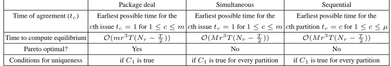
Package deal Simultaneous Sequential Time of agreement (tc) Earliest possible time for the Earliest possible time for the Earliest possible time for the
cth issuetc= 1for1≤c≤m cth issuetc= 1for1≤c≤m cth partitiontc=cfor1≤c≤µ
Time to compute equilibrium O(mr3
T(Nr−T
2)) O(M r
3
T(Nr−T
2)) O(M r
3
T(Nr−T 2))
Pareto optimal? Yes No No
Conditions for uniqueness ifC1is true ifC1is true for every partition ifC1is true for every partition
Table 1. Outcomes for the incomplete information setting –mis the total number of issues and Mis the number of issues in the largest partition (for a definition ofC1see Theorem 3).
to SEQ negotiation for two pies. This model assumes complete information, imposes an agenda exogenously, and studies the relation between the agenda and the outcome of the SEQ bargaining game. On the other hand, [11, 13, 7] study negotiations with an endogenous agenda. For instance, [11] studies PD, SIM, and SEQ negotiation by as-suming complete information. Furthermore, the agents are assumed to have discount factors but no deadlines. The main result of this work is that the PD is the optimal pro-cedure and that for each propro-cedure there exist multiple equilibria. [13] extends this work by finding conditions under which the equilibrium is unique. [7] developed an asym-metric information model for two issues and studied the PD and the SEQ procedure. A slightly different approach was taken in [8] by adding a preliminary period in which agents bargain over an agenda first and then settle the issues using this agenda. How-ever, in [7] and [8] the players have discount factors but no deadlines. In summary, the above work differs from ours in that we consider both discount factors and deadlines, whereas previous work only considers discount factors and no deadlines4. Negotiation
with deadlines was studied in [9] but only for a single issue. Also, the existing litera-ture does not compare the different procedures in terms of a comprehensive list of their attributes (viz. time complexity, Pareto optimality, uniqueness, and time of agreement). Our comparative study of these attributes allows a more informed choice to be made about which procedure is most suitable in which circumstances.
6
Conclusions and future work
This paper analysed the three key procedures for bilateral multi-issue negotiation be-tween self-interested agents: the PD, the SIM, and the SEQ procedures. Our results (see Table 1) show that the PD is better than the other two because it is the optimal pro-cedure for both agents, it is the only one to generate a Pareto optimal outcome, and it achieves these with polynomial time complexity (as the other two procedures). With regard to the time of agreement, the PD and the SIM procedures are similar in that, for the complete information setting, both procedures result in an agreement att = 1for all the issues. Also, when there is uncertainty about deadlines, the earliest possible time of agreement is the same for both procedures. But the SEQ procedure is slower in terms
4
[image:13.612.131.523.68.135.2]of the time of agreement. Finally, all the three procedures have a unique outcome under certain conditions.
In future, we will extend our symmetric information analysis by studying asymmet-ric information settings. Also, in this work, we modelled the players’ time preferences in the form of discount factors. However, it has been shown that the outcome for nego-tiation with discount factors can differ from that for fixed time costs [8]. Therefore, it will be interesting to extend our analysis to negotiations with fixed time costs.
Acknowledgements
We are grateful to Sarit Kraus for her detailed comments on earlier versions of this paper.
References
1. I. Stahl, Bargaining Theory, Economics Research Institute, Stockholm School of Economics, Stockholm, 1972.
2. A. Rubinstein, Perfect equilibrium in a bargaining model, Econometrica, 50(1):97–109, Jan-uary, 1982.
3. C. Fershtman, The importance of the agenda in bargaining, Games and Economic Behavior, 2:224–238, 1990.
4. S. Martello and P. Toth, Knapsack problems: Algorithms and computer implementations, (Chapter 2), John Wiley and Sons, 1990.
5. J. S. Rosenschein and G. Zlotkin, Rules of Encounter, The MIT Press, 1994. 6. M. J. Osborne and A. Rubinstein, A Course in Game Theory, The MIT Press, 1994. 7. M. Bac and H. Raff, Issue-by-issue negotiations: the role of information and time preference,
Games and Economic Behavior, 13:125–134, 1996.
8. L. A. Busch and I. J. Horstman, Bargaining frictions, bargaining procedures and implied costs in multiple-issue bargaining, Economica, 64:669–680, 1997.
9. T. Sandholm and N. Vulkan, Bargaining with deadlines, In Proceedings of the National
Con-ference on Artificial Intelligence (AAAI’99), pages 44–51, Orlando, FL, 1999.
10. C. Fershtman, A note on multi-issue two-sided bargaining: bilateral procedures, Games and
Economic Behavior, 30, 216–227, 2000.
11. R. Inderst, Multi-issue bargaining with endogenous agenda, Games and Economic Behavior, 30: 64–82, 2000.
12. S. Kraus, Strategic negotiation in multi-agent environments, The MIT Press, Cambridge, Massachusetts, 2001.
13. Y. In and R. Serrano, Agenda restrictions in multi-issue bargaining (II): unrestricted agendas,
Economics Letters, 79:325–331, 2003.
14. T. H. Cormen and C. E. Leiserson and R. L Rivest and C. Stein, An introduction to
algo-rithms, The MIT Press, Cambridge, Massachusetts, 2003.