COMPLEX BRAIN NETWORKS
JONATHAN J. CROFTS1 AND DESMOND J. HIGHAM1
Abstract. Recent advances in experimental neuroscience allow non-invasive studies of the white matter tracts in the human central nervous system, thus making available cutting-edge brain anatomical data describing these global connectivity patterns. Via magnetic resonance imaging, this non-invasive tech-nique is able to infer a snap-shot of the cortical network within the living hu-man brain. Here, we report on the initial success of a new weighted network communicability measure in distinguishing local and global differences between diseased patients and controls. This approach builds on recent advances in net-work science, where an underlying connectivity structure is used as a means to measure the ease with which information can flow between nodes. One advan-tage of our method is that it deals directly with the real-valued connectivity data, thereby avoiding the need to discretise the corresponding adjacency ma-trix, that is, to round weights up to 1 or down to 0, depending upon some threshold value. Experimental results indicate that the new approach is able to extract biologically relevant features that are not immediately apparent from the raw connectivity data.
1. Motivation
In recent years complex networks have received a significant amount of at-tention (Albert & Barabasi 2002, Newman 2003, Strogatz 2001). The need to study apparently disparate real-world networks using a single unified language has led to the growth of an interdisciplinary field that involves mathematicians, physicists, computer scientists, engineers and researchers from both the natural and social sciences. In this work we are interested in nature’s most complex system, the human cerebral cortex (Sporns & Zwi 2004). The development of diffusion magnetic resonance imaging (MRI) has enabled neuroscientists to con-struct connectivity matrices for the human brain and ‘proof of principle’ work has shown that existing biological knowledge can be recovered from this connectivity data (Klein et al. 2007).
Our ability to understand and compare different connectivity structures can be greatly facilitated by the introduction of easily computable measures that characterise the network topology. Typically, measures of this type rely heavily
Date: December 8, 2008.
Key words and phrases. matrix functions, network science, neuroscience, unsupervised classification.
on the idea that communication, to be understood here as the ease of infor-mation spread between nodes on the network, takes place along geodesics. How-ever, in many real-world networks information can disseminate along non-shortest paths (Borgatti 2005, Newman 2005) and for such networks any meaningful mea-sure of ‘communicability’ should account not only for the shortest path between two nodes, but also all other possible routes. Motivated by this consideration, Estrada & Hatano (2008) recently advanced a new definition of communicabil-ity that takes non-shortest paths into account with an appropriate length-based weighting. This definition applies to networks with unweighted edges. In the case where the connectivity information is real-valued, converting this informa-tion into the required binary format is undesirable because (a) it requires a cutoff value to be determined and (b) fine details about connectivity strengths are lost. This report has two main aims: (i) introduction of a new, computable measure of connectivity for a weighted network, and (ii) application of this new measure
to the case of cutting edge anatomical connectivity data for the brain. In§2 we
develop the new measure by extending the definition of communicability to the case of weighted networks, taking care to deal with the issue of normalisation. We then present a comparison of connectivity data for stroke patients and healthy
control subjects in§3.
2. Network Communicability
Suppose we are given a network consisting of (a) a list of nodes and (b) a list of edges connecting the nodes. In the language of graph theory, this is an undirected, unweighted graph that could be defined in terms of the adjacency
matrix A ∈ RN×N
, which has aij = aji = 1 if nodes i and j are connected and
aij =aji = 0 otherwise. We will always set aii = 0, so that self-links, also called
loops, are disallowed. Estrada & Hatano (2008) recently put forward the concept
of communicability to address the issue that the existence or nonexistence of
an edge does not necessarily capture the degree of “connectedness” between a pair of nodes. For example two nodes that are not themselves connected, but have many neighbours in common should be regarded as closer together than two unconnected nodes that can only be joined through a long chain of edges. An
extremely useful observation is that if we raise the adjacency matrix to the kth
power, then itsi, jth element
(1) Ak
ij := N
X
r1=1
N
X
r2=1 . . .
N
X
rk=1
ai,r1ar1,r2ar2,r3. . . ark
−1,rkark,j,
counts the number ofwalks of length k that start at nodei and finish at nodej.
Here the termwalk refers to any possible traversal through the network that
fol-lows edges, andlength refers to the number of edges involved. Estrada & Hatano
summing the number of walks of length 1,2,3, . . .. Because short walks are more important than long walks, for example in a message-passing scenario shorter
walks are faster and cheaper, to arrive at a single real number walks of lengthk
are penalised by the factor 1/(k!). This leads to a definition of communicability
between nodesiand j, fori6=j, given by P∞
k=1Ak/(k!)
ij, or, more compactly,
exp(A)ij (Estrada & Hatano 2008). We also note that in addition to giving a neat
characterisation in terms of the matrix exponential, the choice of scaling factor
k! can also be justified from the perspective of statistical mechanics (Estrada &
Hatano 2007) .
In our context, the connectivity information arises in the form of real-valued,
non-negative weights, where a larger weight aij indicates that nodes i and j are
more strongly connected. The identity (1) remains valid in this more general setting, but now the termai,r1ar1,r2ar2,r3. . . ark
−1,rkark,j does not give a zero/one
contribution depending on whether the walk i7→ r1 7→r2 7→r3 7→ · · · 7→ rk 7→j
is possible. Instead it contributes the product of the weights along all the edges in the walk. Downweighting the contribution of longer walks is especially relevant here, since experimental uncertainty generally increases with length.
Although it is appealing to use exp(A) in this way to define communicability
for a weighted network, such a measure is likely to suffer from difficulties if the weights are poorly calibrated. A highly promiscuous node with large weights is liable to have an undue influence. Similar effects have been observed in the con-text of spectral clustering (Higham, Kalna & Kibble 2007), where it has proved successful to judge the size of a cluster not by the number of nodes, but by the total weight of connections that they possess. This results in a natural
nor-malisation step in which the weight aij is divided by the product
p
didj, where
di :=
PN
k=1aik is the generalised degree of node i. An example illustrating the
benefits of this normalization step can be seen in§3.2. By analogy, we therefore
define the communicability between distinct nodesiandj in a weighted network
by
(2) expD−1
2AD− 1 2
ij,
where the diagonal degree matrix D∈RN×N
has the form D:= diag(di).
In the next section we show that this new measure extracts useful information from brain connectivity networks.
3. Brain Network
0 5 10 15 20 −0.5 −0.4 −0.3 −0.2 −0.1 0 0.1 0.2 0.3 0.4 Raw V [2]
0 5 10 15 20 −2 −1.5 −1 −0.5 0 0.5 1
x 10−3Normalised
D
−1/2 right
V
[2]
n
[image:4.612.135.449.50.257.2]0 5 10 15 20 −0.6 −0.5 −0.4 −0.3 −0.2 −0.1 0 0.1 0.2 0.3 0.4 Communicability V [2]
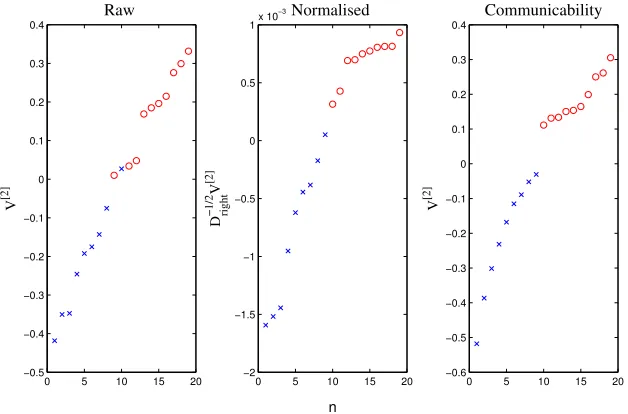
Figure 1. Components corresponding to stroke patients are la-beled with crosses and circles denote controls. Left: components of
the right singular vector, v[2], of the original data matrix. Centre:
components of the scaled right singular vector D−
1 2
rightv[2]. Right:
components of the second right singular vector, v[2], of the data
matrix after post-processing using communicability.
(mesoscale); and (iii) anatomically distinct brain regions and corresponding inter-regional pathways (macroscale). In this work, due to the resolution limits of MRI data, we focus on the macroscale description of the human brain. We define a network using the Harvard-Oxford cortical and subcortical structural atlases as implemented in fslview, part of FSL (Smith et al. 2004), thereby partitioning the brain into 56 anatomically distinct regions—48 cortical and 8 subcortical. This produces a weighted, undirected graph with 56 nodes. In our experiments, we have structural diffusion weighted imaging data for 9 stroke patients (at least six months following first, left hemisphere, subcortical stroke) and 10 age matched controls.
A more detailed description of the materials and methods is provided online; see Appendix A.
3.2. Spectral clustering. We set ourselves the task of unsupervised clustering of the patients, to check how accurately we can recover the known stroke/control
groupings. A patient data set consists of (562 −56)/2 = 1540 distinct values,
giving the connectivity strength between each pair of distinct brain regions. We
used each of the 19 patient data sets to create the columns of a matrix W ∈
R1540×19
regions in patientj. Unsupervised clustering on the 19 columns of this matrix was performed using the singular value decomposition (SVD) (Higham et al. 2007). This approach is closely related to many other techniques, such as Principal Components Analysis, support vector machines/kernel based methods, machine learning and multidimensional scaling (Cox & Cox 1994, MacKay 2003, Skillicorn 2007).
The second right singular vector,v[2] ∈R19, can be used to assign a value v[2]
j
to the jth patient, and the aim is that patients with similar connectivity profiles
will be assigned nearby values. This is a classical dimension reduction technique, where a vast amount of information is compressed into a single one-dimensional summary that is much easier to visualize and interpret. In particular, a large gap between successive components, especially a gap that straddles the origin, is an indication that the nodes on either side are members of distinct subgroups.
The left hand picture in Figure 1 shows the values of v[2], plotted in
increas-ing order. Components correspondincreas-ing to stroke patients are labeled with crosses and circles denote controls. We see from the picture that although the SVD has placed the strokes and controls approximately in order, a stroke and control (in positions 9 and 10) have been misordered and there is no clear gap separating strokes and controls. The middle picture in Figure 1 shows the
correspond-ing plot when the SVD is applied to the normalised data matrix D−
1 2
leftW D
−1 2
right,
with (Dleft)i :=
P19
j=1wij and (Dright)j :=
P1540
i=1 wij, and the normalized left
sin-gular vector D−
1 2
rightv[2] is displayed, as discussed for the case of microarray data
in (Higham et al. 2007). We see that the classification is improved by the normal-isation process in the sense that strokes and controls appear sequentially. Closer inspection of the raw data showed that for the two patients that were originally ordered incorrectly, one had unusually large and the other had unusually small
overall connectivity weights, (Dright)i; this is precisely the situation where
nor-malisation is designed to be beneficial. We note, however, that nornor-malisation has not dealt successfully with the separation issue. There is no obvious gap between strokes and controls, and a cut-off at the origin would place a stroke among the controls.
3.3. Communicability. We motivated the new weighted communicability mea-sure by arguing that the higher order terms in the power series of equation (2) con-tain important additional information. We now provide evidence that weighted communicability does indeed add value to the raw data.
3.3.1. Spectral clustering based on weighted communicability. We now repeat the
unsupervised clustering task for the new data matrix, C ∈ R1540×19
, whose columns are constructed from the respective communicability networks, so that
cij gives the communicability strength for the ith pair of brain regions in
singular vector,v[2], plotted in increasing order. We see that post-processing the data using communicability significantly improves the results of the clustering algorithm, giving a correct ordering and a clear separation, with the two groups having opposite signs; negative for strokes and positive for controls. Using the
second left singular vector, u[2], we may proceed to identify those connections
that enable us to distinguish between stroke and control classes; further details are provided in the supplementary material.
3.3.2. Statistical Validation. To quantify the effect of using weighted
commu-nicability, we applied the mean-centred partial least squares (PLS) approach of McIntosh and colleagues (McIntosh & Lobaugh 2004). Via the SVD, PLS analysis returns latent variable pairs (left/right singular vectors containing the connection/group saliences) which describe a particular pattern of connectivity covariance according to subject. The statistical significance of each latent variable was determined using permutation tests of 500 permutations, whilst the reliabil-ity of saliences of the individual connections in contributing to the pattern of covariance identified by the latent variables was determined using 100 bootstrap analyses.
The PLS analysis returned one significant (p ≤ 0.01) latent variable pair for
each of the three data sets described above. In each case PLS was able to distin-guish between stroke and control classes, however, this should not be to surpris-ing since PLS is a supervised method. Perhaps more importantly, the number of connections which returned saliences in the 99th percentile was greatest for com-municability (318), then the normalised data (290) and lowest in the raw data (266); suggesting that communicability has the effect of reducing the influence of noise in the data.
4. Discussion
Our new network measure extends the concept of communicability in a nat-ural manner to the case of weighted networks. Initial tests reported here on cutting-edge anatomical brain connectivity data show that this measure can give statistically significant enhancement to the performance of standard data analy-sis tools. In future work we plan to study networks relating to a range of brain disorders and investigate the underlying changes in connectivity structure that are revealed through the new measure.
Acknowldegement
Appendix A. Supplementary data
Supplementary data associated with this article can be found at
http://www.maths.strath.ac.uk/~gcb07174/crofts/rs/rsoc08_supp.html
References
Albert, R. & Barabasi, A. L. (2002), ‘Statistical mechanics of complex networks’,
Rev. Mod. Phys. 74, 47–97.
Borgatti, S. P. (2005), ‘Centrality and network flow’,Social Networks 27, 55–71.
Cox, T. F. & Cox, M. A. A. (1994),Multidimensional Scaling, London: Chapman
and Hall.
Estrada, E. & Hatano, N. (2007), ‘Statistical-mechanical approach to subgraph
centrality in complex networks’, Chemical Physics Letters 439, 247–251.
Estrada, E. & Hatano, N. (2008), ‘Communicability in complex networks’,Phys.
Rev. E 77, 036111.
Higham, D. J., Kalna, G. & Kibble, M. (2007), ‘Spectral clustering and its use in
bioinformatics’, Journal of Computational and Applied Mathematics 204, 25–
37.
Klein, J. C., Behrens, T. E. J., Robson, M. D., Mackay, C. E., Higham, D. J. & Johansen-Berg, H. (2007), ‘Connectivity-based parcellation of human cor-tex using diffusion MRI: establishing reproducability, validity and
observer-independence in BA 44/45 and SMA/pre-SMA’, NeuroImage 34, 204–211.
MacKay, D. J. C. (2003), Information Theory, Inference and Learning
Algo-rithms, Cambridge: Cambridge University Press.
McIntosh, A. R. & Lobaugh, N. J. (2004), ‘Partial least squares analysis of
neuroimaging data: applications and advances’, NeuroImage 23, 250–263.
http://rotman-baycrest.on.ca/index.php?section=84.
Newman, M. E. J. (2003), ‘The structure and function of complex networks’,
SIAM Rev. 45, 167–256.
Newman, M. E. J. (2005), ‘A measure of betweeness centrality based on random
walks’, Social Networks 27, 39–54.
Skillicorn, D. (2007),Understanding Complex Datasets, Chapman & Hall/CRC.
Smith, S. M., Jenkinson, M., Woolrich, M. W., Beckmann, C. F., Behrens, T. E. J., Johansen-Berg, H., Bannister, P. R., Luca, M. D., Drobnjak, I., Flitney, D. E., Niazy, R. K., Saunders, J., Vickers, J., Zhang, Y., Stefano, N. D., Brady, M. J. & Matthews, P. M. (2004), ‘Advances in functional and structural MR
image analysis and implementation as FSL’, NeuroImage 23(S1), 208–219.
Sporns, O., Tononi, G. & K¨otter, R. (2005), ‘The human connectome: a
struc-tural description of the human brain’, PLoS Comput. Biol. 1(4), 245–251.
Sporns, O. & Zwi, J. (2004), ‘The small world of the cerebral cortex’,
Neuroin-formatics2, 145–162.