Ames Laboratory Technical Reports Ames Laboratory
6-1960
An IBM 650 computer program for determining
the thermal diffusivity of finite-length samples
William L. Kennedy
Iowa State University
Follow this and additional works at:http://lib.dr.iastate.edu/ameslab_isreports Part of thePhysics Commons
This Report is brought to you for free and open access by the Ames Laboratory at Iowa State University Digital Repository. It has been accepted for inclusion in Ames Laboratory Technical Reports by an authorized administrator of Iowa State University Digital Repository. For more information,
please [email protected].
Recommended Citation
Kennedy, William L., "An IBM 650 computer program for determining the thermal diffusivity of finite-length samples" (1960).Ames Laboratory Technical Reports. 13.
finite-length samples
Abstract
A new technique has been developed for measuring the thermal diffusivity of finite-length samples. The sample was in the form of a round rod surrounded by a cylindrical guard. Both the sample and the guard had a small heater attached to one end. The heater was turned on and the voltages of equally spaced thermocouples were plotted as a function of time. This procedure determined the boundary conditions necessary for the solution of the heat flow equation. The solution at the sample midpoint was obtained by assuming various values of thermal diffusivity. The value of thermal diffusivity which gave the best agreement between the computed solution at the sample midpoint and the experimental curve obtained at the midpoint was
considered to be the best value for the thermal diffusivity. An IBM 650 computer was used to process the data.
Disciplines Physics
AN IBM 650 COMPUTER PROGRAM FOR ETERMINING THE THERMAL
DIFFUSIV-ITY OF FINITE-LENGTH SAMPLES by
IS-137
Physics and Mathematics (UC-34) TID-4500, August 1, 1959
UNITED STATES ATOMIC ENERGY COMMISSION
Research and Development Report
AN IBM 650 COMPUTER PROGRAM FOR DETERMINING THE THERMAL
DIFFUSIV-ITY OF FINITE-LENGTH SAMPLES
by
William Leon ~ennedy
June 1960
Ames Laboratory at
Iowa State University of Science and Technology F. H. Spedding, Director
Contract W -7405 eng-82
2
IS-137
This report is distributed according to the category Physics and Mathe-matics (UC-34) as listed in TID-4500, August 1, 1959.
Legal Notice
This report was prepared as an account of Government sponsored work. Neither the United States, nor the Commission, nor any person acting on behalf of the Commission:
A. Makes any warranty of representation, express or implied, with respect to the accuracy, completeness, or usefulness of the in-formation contained in this report, or that the use of any informa-tion, apparatus, method, or process disclosed in this report may not infringe privately owned rights; or
B. Assumes any liabilities with respect to the use of, or for damages resulting from the use of any information, apparatus, method, or process disclosed in this report.
As used in the above, "person acting on behalf of the Commission" includes any employee or contractor of the Commission, or employee of such con-tractor, to the extent that such employee or contractor of the Commission, or employee of such contractor prepares, disseminates, or provides access to, any information pursuant to his employment or contract with the Commis-sion, or his employment with such contractor.
\
Printed in USA. Price $ 1. 50 Available from the
I$ - 137 CONTENTS
Page
Abstract . . . , . . . 5
Introduction . . . . . . . . . . . . . . . . . . . . . . 5
1. The General One-dimensional Heat Flow Problem... 6
2. Experimental Technique for Determining Thermal Diffusivity . . . 7
3. Discussion of the Computer Program 3. 1 Method of Solution . . . , . . . 8
3. 2 General Operation of the Program . . . 11
3. 3 Sequence of Data Cards . . . 13
3. 4 Output Card Format . . . 15
3. 5 Minimum Equipment . . . 16
3. 6 533 Control Panel . . . 16
4. Thermal Diffusivity of Armco Iron . . . 16
5. Conclusion . . . · . . . 20
6. Acknowledgment . . . , . . . 22
APPENDIX I. Program Block D~agram . . . • . . . 22a II. Program . . . 23
III. Standard SO-Column Listing of the Program Decks . . . • . . . 40
IV. Example Data and Output . . . 56
AN IBM 650 COMPUTER PROGRAM FOR DETERMINING THE THERMAL DIFFUSIVITY OF FINITE-LENGTH SAMPLES
William Leon Kennedy
ABSTRACT
A new technique has been developed for measuring the thermal diffu
-sivity of finite-length samples. The sample was in the form of a round
rod surrounded by a cylindrical guard. Both the sample and the guard
had a small heater attached to one end. The heater was turned on and the
voltages of equally spaced thermocouples were plotted as a function of time.
This procedure determined the boundary conditions necessary for the
solu-tion of the heat flow equasolu-tion. The solution at the sample midpoint was
obtained by assuming various values of thermal diffusivity. The value of
thermal diffusivity which gave the best agreement between the computed
solution at the sample midpoint and the experimental curve obtained at the
midpoint was considered to be the best value for the thermal diffusivity.
An IBM 650 computer was used to process the data.
INTRODUCTION
High-speed computers have made it possible to ap:proach many problems
in a manner that would not be feasible by the use of ordinary desk calculators.
In the case of thermal diffusivity measurements, it has been the custom to
choose a sample geometry that will give a solution of the heat-flow equation
;;;\\hlch is easily calculated by ordinary methods. The geometry commonly
6
This new method considers a sample of finite length. A basic machine language program for the IBM 650 computer has been developed in order to process the data. This program utilizes fixed-point arithmetic.
1. The General One-dimensional Heat Flow Problem Consider a homogeneous rod of constant cross-sectional area A.
Suppose that the sides are insulated so that the streamlines of heat flow are all parallel, and perpendicular to the area A. It can be shown1 that the partial differential equation desc:dbing the temperatu<re of such a rod as a function of both displacement and time is
au
at
where u
=
temperature (arbitrary units), k ::;;: thermal diffusivity ( cm 2 /sec ). andInformation concerning the initial and boundary conditions is required in order to obtain a general solution of the form u = f(x, t). The initial condition for the general problem is
u( x, t =
0 )
= g(x) for 0 < x < L. The boundary conditions areu( x
=
0, t=
<j>(t) and u( x=
L, t=
~(t)for t > 0.
If the thermal diffusivity (k) of the rod and the above initial condition
and boundary conditions are known, it is possible to obtain the general solution u = f(x, t).
2. Experimental Technique for Determining_ Thermal Diffusivity
A rod- sl:\p.ped sample was constructed with a small heater fixed to one
end. Surrounding the sample and also attached to the heater was a cylindrical
guard fabricated from the same material as the sample. The purpose of
this guard was to reduce radial heat losses. by radiation. Three
thermo-couples were located at equal intervals along the sample. The
thermo-couple located closest to the heater was designated to be at x = 0. The
distance between the extreme thermocouples was L em. The heater was
turned on at t = 0. The thermocouple voltages were plotted independently
as a function of time. The entire sample was assumed to be at ambient
temperature at t = 0. This assumption implies that the initial condition
is u(x, t = 0) = g(x) =a constant. The constant was chosen to be zero
since the reference point for a temperature scale is arbitrary. ·The heat
flow equation can be solved subject to the two boundary conditions determined
by the x = 0 and x
=
L thermocouples. A solution u{x =~,
t) =~(t)
at the sample midpoint could be obtained provided that the thermal
diffu-sivity (k) of the rod is known. The thermal diffusivity (k) was varied
until the best agreement was obtained between the computed solution at
the sample midpoint and the experimental curve given by the midpoint
thermocouple. This experimental curve was designated as u(x =
~,
t) =a
(t). The expression[ ~(t)]. - [
a
(t)] . = £.1 1 1
is the difference between the computed curve and the experimental curve
for a given time t . .
8
The mean squared error
2
[N
2l
s =
i~l
£iJ
I
Nwas computed over the range 0 < t < t for each trial value of thermal max
diffusivity (k). The value of k which made the:,mean sqgared error a minimum
was assumed to be the best estimate of the sample 1 s thermal diffusi vity
at a given temperature. The sample temperature was taken to be the
temperature at t = 0 since at t the temperature at x = 0 was only about max
1
oc
above the ambient temperature.The mean squared error was minimized rather than the raw sum of
the deviations sqruared since N is a function of the thermal diffusivity.
This procedure was used owing to the method employed to solve the heat
flow equation. This method will be discussed in the next section. The
experiment is summarized in Figs. 1 and 2.
3. Discussion of the Computer Program
3. 1 Method of Solution
The differential equation was solved by the method of finite differences. ('
The difference equation2 employed was
u(x, t+~t) = 1 [ u(x+~x, t) + 4u(x, t) + u(x-~x. t)) b
where
~t
=
L2 n = 2, 4, 6,....
~n2k
and
~X = L
n
2 For a derivation of this equation and a discussion of the errors involved,
sree lNumerical Solution~ Differential Equations by W. E. Milne, (John
Wiley and Sons, 1953). p. 119.
t(l
\ I Q)
s
...
...
~I
@
...
Q) p,.s
reiCD Q)
...c:
-
...
u
b.OlOW ~
- ( f ) 0
-
Cd-
w
CD-
~ ~...
~
-
-
:E
~-
Q:)...
....
... 0-e-
II II p,.II
-
-~ ~ 0 (I)
-
~..
::I0
..
_JjC\J _J ...0 ,...
II II II rei
) ( ) ( ) (
>
-
:::J-
:::J-
:::J...
rei(I) 10 Q) ,...
3
rei
,...
CJj
p,.
s
Q)
0 ~
0 0 0 0 0 0 0
0 0 0 0 0 0
...
"" C\J
o
·
oo
w
v
C\J0
\ b.O
5.00
~--,.---,r---r---..,.---r----r---r----r----n----,
4.00
3.00
C\Jcn
2.00
1.00
o.oo~--~--~--~--~--~--~~~~--~--~'
0.120
0.122
.
0.124
0126
0.128
0.130
THERMAL
DIFFUSIVITY
.
(CM
2
/SEC)
E:;ig.
2.
Mean
squared
error~
thermaldiffusivity.
~
It can be seen that ~t depends upon the thermal diffusivity of the sample
and the length of the sample. Five ~x routines were written in order to
accommodate samples of different lengths and thermal diffusivities. These
five x-mesh size routines corresponded to n = 2, 4, 6, 8, and 10.
3. 2 General Operation of the Program
The program is divided into two parts. The main program deck, a
seven instruction per card deck, is loaded first. The desired x-mesh size
deck is placed immediately behind the main program deck. All x-mesh
size decks are made up of single instruction load cards.
Since the program is self-initializing and self-initiating, the sets of
data cards may be placed directly behind the program decks. The sets of
data must be arranged in either ascending or descending temperatures.
This arrangement is necessary since the computer uses the previously
determined value of k as the starting estimate of k for the next data
set. Therefore, an estimate of k is supplied by means of a punched card
for only the first set of data. The computer minimizes the mean squared
error by stepping kin increments of 0. 001 cm 2 /sec. This increment is
stored in location 0917. For high thermal diffusi vity materials it might be
desirable to change this to a larger increment. The format of the increment
is 00000. NNNNN.
As the program is now written the initial conditions are loaded by the•
program. The temperature distribution before heat is applied to the heater
is considered to be a constant (ambient temperature). Therefore, zeros
are loaded by the program for the initial temperature distribution. However,
12
other than zeros as part of the data. A no-operation instruction has been
written in the data load routine (see Appendix I) that could be replaced by
a subroutine to read in the initial conditions. The initial conditions are
presently found in the x-mesh size routines.
The console settings for this program are:
Storage Entry Switches: 70 1951 XXXX +
Programmed Switch:
Half Cycle Switch:
Address Selection Switches:'
Control Switch:
Display Switch:
Overflow Switch:
Error Switch:
Stop
Run
xxxx
Run
Program Register
Sense
Stop
This pro-gram contains only one programmed stop. If the estimate for
k is quite different from the true value of k, the machine will stop and
display 01 0000 0652+. If this occurs, one should set up a better estimate..-
-for k on the storage entry switches and depress the program start key.
The format of k is OOOON, NNNNN.
If one should want to read in a different estimate for k at any time,
it can be done in the following manner without reloading the program or
the data, Depress the program stop key. Set the storage entry switches to
00 0000 0075+. Depress the computer reset key and then depress the
program start key for an instant. The display lights should now read
01 0000 0 174+. -At this point the new estimate for k is entered on the
computer to start calculating on the basis of the new estimate for k. This procedure could be very helpful when starting if one is working on a material for which the thermal diffusivity is completely unknown.
It is possible to read in data cards without reloading the program
by the following procedure. Set the storage entry switches to 00 0000 0650+. Then depress the computer reset key. A depression of the program start key will read in data cards and execute the program. This procedure
includes reading the k estimate card. If the machine contains an estimate
for k and it is not necessary to read the k estimate card, set the storage entry switches to 00 0000 0553+, and follow the above procedure.
3. 3 Sequence of Data Cards Card 1
Word 1 - An estimate for the thermal diffusivity (k) for the first set of data. The format is OOOON. NNNNN. The remainder of this card is blank. This card is required only for the first temperature point since the succeed-ing points derive their estimates fork from the precedsucceed-ing points.
Card 2
Word 1 - Temperature. The format is ONNNN. NNNNN .
. Word 2 - The constant which all of the ordinates of the experimental curve
obtained at the sample midpoint must be divided by in order to place this
curve on the same scale as the experimental curve obtained at x
=
0. Theformat is OOONN. NNNNN.
Word 3- The constant which all the ordinates of the experimental curve
obtained at x = L must be divided by in order to place this curve on the same
. 14
Note: Even if the ordinates of the exper~ental curve obtained at x = L
are .all zero~ this constant must be non-zero in order to prevent a machine
stop caused by a division overflow.
Word 4- t for the experimental curves minus AT. The unit for this
max
quantity is seconds. The format is OONNN. NNNNN. Note: t must be
max
equal to nATwhere n is anyi nterger.
Word 5- The uniform interval between the absissas of all curves (A1).
The unit are. seconds. This interval should be small enough so that a
linear interpolation between successive coordinates of each curve is a
good approximation. The format is OOONN. NNNNN.
Word 6 = L 2. The format is OONNN. NNNNN. The units for this quantity
2
are em .
Word 7 = Blank.
Word 8 = Card identification if desired. The format is NNNNNNOOOO.
Cards 3 - ll (9 cards)
These cards contain the ordinates for the experimental curve obtained at
x
=
0. The first ordinate is for t=
0 . . The ordinates. are loaded in ascendingorder for absissas A'T apart. If all 72 words ar e not used~ the remaining
words must be filled with zeros. The format i OOOOOONNNN.
Cards 12 =· 20 .(9 cards)
These cards contain.the ordinates.for the experimental curve obtained at
L
x
=
2
.
.
The conditions imposed on cards 3 = 11 also apply for this set.Cards 21 - 29 (9 cards)
These cards contain the ordinates for the experimental curve obtained at
It is imperative that these data cards be in the order as given.
Columns 71 - 76 inclusive on all data cards may be used for the purpose
of card identification. However, these columns must be filled. Multiple
punches are not allowed in these columns.
Up to 72 coordinate pairs are allowed for each experimental curve,
including the origin. The origin must always be included. There must be
the same fixed interval between the absissas of all three experimental
curves. This absissa interval is designated as ~T, and should not be confused
with ~t. The choice of ~Tis arbitrary. However, ATmust be small enough
so that a linear interpolation between consecutive coordinates on the
experimental curves is valid.
The ordinates of each experimeP,.tal curve can be measured from an
arbitrary reference line below the origin of the curve. The computer
subtracts the value of the origin ordinate from all other ordinates on the
curve before they are stored. This feature is desirable if the ordinates
are measured.by some of the chart measuring devices that are available.
3. 4 Output Card Format
The output consists of only one type of card.
Word 1 - Temperature. The format is ONNNN. NNNNN.
Word 2 - Thermal diffusivity (k). The units are em /sec and the format 2
>
is OOOON. NNNNN.
2
Word 3 - Mean squared error (s ). The format is OOOONNNN. NN.
Word 4 - x-me·s.h size (n). The format is OOONN. NNNNN.
Word 5 - The computed t-mesh size (~t). The format is OOONN. NNNNN.
Word 6 - The number of points used in computing the mean squared error
16
Word 7 - Zero.
Word 8 - Zero.
For a given temperature, the thermal diffusivity (k) is plotted as a
function of the.mean squared error (s 2 ). The value of k for which s 2
is a minimum is considered to be the thermal diffusivity of the sample at
the given temperature (Fig. 1). See Appendix IV for example .dataand output.
3. 5 Minimum Equipment
The minimum equipment for this program is a basic 2000 ward IBM
650 computer with a 533 input-output unit. No special devices are required.
3. 6 533 Control Panel
The 533 control panel is wired for standard ten digit, eight wor~
input and output operation. The read validity check switch is jack-plugged
off in order to avoid having .to punch the unused wortl fields on the. data cards.
Since the data are all positive, it is advantageous to leave the read plus
sign switch unwired. · A load card is designated by a 12-punch in column 1.
4. Thermal Diffusivity of Armc~,Iron
Data was obtained for armco iron from 309°C to lll2°C at small in
-tervals of temperature in order to evaluate this new method. Armco iron
was chosen for several reasons. There w~re other thermal diffusivity
data available for armco iron that could be used for a compar-ison. The
thermal diffusivity of armco iron changes rap~ly with temperature in the
vicinity of the Curie .temperature (770 o C). It was felt that a method giving
good results in this region would have merit. The thermal diffusivity of
iron is low compared to many metals. ·Calculations proved that it would be
possible to use only two thermocouples if L was about 2 1/2 em and t
max
an insignificant temperature increase compared to the thermocouple located at x = 0 by the time t = t . This calculation was based on the value of
max
the thermal diffusivity of iron at 300°C. The thermal diffusivity of iron decreases rapidly for temperatures higher than 300°C. The assumption that at x = L the temperature does not rise appreciably above the ambient temperature for a small t is certainly valid for sample temperatures
max
greater than 300°C. However, since there was no thermocouple at x
=
L, precision had to be sacrificed in order to insure accuracy at the lower temperatures. This was due to the fact that a t had to be used thatmax
was less than the actual t for the experimental curves. Therefore, max
the available experimental data was reduced. It is believed that it would always be beneficial to the experiment to include a thermocouple at x = L, even if the sample were a poor thermal diffuser.
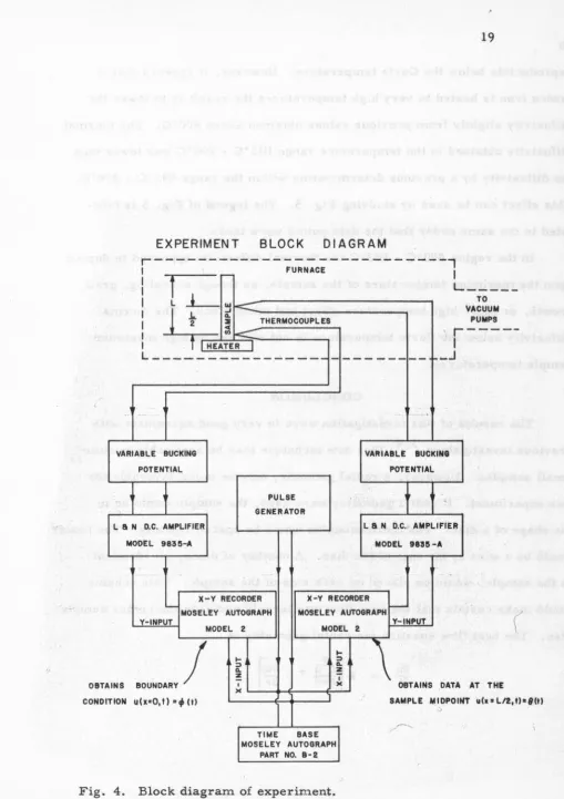
The sample design is illustrated in Fig. 3. A block diagram of the experimental apparatus is shown in Fig. 4. The heater, the time base, and the pulse generator are started simultaneously. The pulse generator causes a small spike to be superimposed on the continuous experimental curves at one-second intervals. The ordinates can then be read directly without having to calibrate the time base. The problem of time base non-linearity is eliminated by this scheme.
The thermal diffusivity of armco iron as a function of temperature is shown in Fig. 5. The results of this investigation agree very well with previous investigators. 3 • 4 The thermal diffusivity of armco iron is quite
3 P. H. Sidles and G. C. Danielson, private communication, Ames
Laboratory, U.S.A.E.C. , Ames, Iowa.
4
.
,
SAMPLE
DESIGN
r---;==
AL
2
o
3
TUBING
ARMCO
IRON
GUARD
ARMCO
IRON
SAMPLE
--THERMOCOUPLES
SHELDS
HELIARC
WELD
.--REFRACTORY
CEMENT
Fig.
3
.
Sample
·
design
.
EXPERIMENT
BLOCK
DIAGRAMr---1
1 FURNACE I
I
f
r--I L
I L
j__~f<
I
~
~
THERMOCOUPLES
I ~
k:::::"
\
r
I
I ATER I
I
L---
---
--
... J
--VARIABLE BUCKING VARIABLE BUCKING
POTENTIAL POTENTIAL
PULSE ~
--, GENERATOR
LaN D.C. AMPLIFIER L6N D.C.;-AMPLIFIER
MODEL 983!5-A MODEL 98311-A
-
-X-Y RECORDER X-Y RECORDER
'--MOSELEY AUTOGRAPH MOSELEY AUTOGRAPH
1--Y-INPUT Y-INPUT
MODEL 2 MODEL 2
...
...
~~ 0.
0. !
z
-
I'rO VACUUM
PUMPS
OBT A INS BOUNDARY
J
I ) ( \ OBTAINS DATA AT THE)(
(
COND IT ION u(x•O,t) · • (I) SAMPLE MIDPOI NT u!x•LI2,tJ•9(t)
:,
,-... .
-TIME BASE /
MOSELEY AUTOGRAPH PART NO. B-2
[image:22.601.75.585.41.763.2]20
reproducible below the Curie temperature. However, it appears that if armco iron is heated to very high temperatures the result is to lower the diffusivity slightly from previous values obtained above 800°C. The thermal diffusivity obtained in the temperature range 1112
oc -
800°C was lower than the diffusivity by a previous determination within the range 993°C - 800°C. This effect can be seen by studying Fig. 5. The legend of Fig. 5 is tabu-lated in the same order that the data points were taken.In the region 800°C - lll2°C the thermal diffusivity appeared to depend upon the maximum tempel,"ature of the sample, as though annealing, grain growth, or other high temperature effect h~d taken place. The thermal diffusivity below the Curie temperature is not effected by_ high maximum
'
sample temperatures.
· CONCLUSION
The results of this investigation were in very good agreement with previous investigators. 3 ' 4 This new technique may be applicable to quite small samples. However, a radial geometry may be more favorable for
. this experiment. If radial geometry were used, the sample would be in
the shape of a disc. The thermocouples would be spaced radially. The heater would be a wire at the axis of the disc. A number of discs, all identical
to the sample, would be placed on each side of the sampr~. This scheme would make certain that the heat flow was largely radial in the center sample disc. The heat flow equation for radial geometry is
au
\
'
o.ts
1
--,----,---.---r---.--.--.,---.,...--r---u
~
(\I'
0.12
~ (.)
-
>-
t->
(/)~
0.08
LL.
0
...J~
0::~0.04
t-RESENT
INVESTIGATION
..
831
-992°C.
o
965-315°C.
a
309-II
I2°C.
•
1088-350°C.
•
IOII-325°C.
ARMCO
IRON
&
o
o6
4
a
a
11
_
~~
I
pA
&
&
..
'
0.00200
400
600
800
1000
TEMPERATURE
(°C)
Fig.
5.
Thermal
diffusivity
,
of
armco
iron~
temperature.
22
Sample fabrication would be simplified considerably for the proposed radial
geometry experiment.
It is difficult to calculate just exactly how well the cylindrical guard
reduced radial heat losses of the sample at high temperatures, However,
the results obtained for armco iron were in ver:>r good agreement with the
results obtained by methods which included a radial heat loss term in the
heat flow equation. It is concluded that radial heat losses are not a serious
source of error if the sample is guarded by a cylindrical guard fabricated
from the sample material.
6. Acknowledgments
The author wishes to express his appreciation to Dr. G. C. Danielson
and Mr. P. H. Sidles for many helpful discussions concerning the general
heat flow problem and experimental techniques, . to Dr .. H. 0. Hartley for
a discussion of the numerical solution of the heat flow equation, to Mr .. H.
W. Jespersen and Mr. Russell Altenberger for many helpful suggestions
for the computer program, to Mr. Garry Wells and Mr. 0. M. Sevde
for fabricating the armco iron sample, and to Mrs. Evelyn Blair for doing
START
READ
AN
ESTIMATE
FOR k
.
INITIALIZE
AND
LOAD
DATA.
INCREASE
k
BY
flk.
COMPUTE
flt.
SET
1:
•
0.
SET
N
=
0.
INCREASE t
BY
~t.
IS
t
>
PROGRAM
BLOCK
DIAGRAM
\----..!
STORE
s?
SET flk
=
-flk.·~
<
·~
?
IS
sj
?
(j=
3,4,5.-··) STORE
2
82
COMPUTEf
E·
II
.,,
s2-L!.L
NJ+l.
PUNCH
2
TEMP,
k
,
s
,
n
,
~t
,
AND
N
•
TABLE
LOOKUP:
FIND
.(t)
,9ttl,
AND
t(tl
.
INCREASE
N
BY
I.
EVALUATE
u
(
x,
t
+tlt.)
.
N
COMPUTE
E~
AND
ACCUMULATE
.L€~.
t•lOF
k
?
"
STORE
STORE s2
I
23
APPENDIX II--PROGRAM LISTING
MAIN PROGRAM
NO LOCN CONTENTS REMARKS
1 001 0650 70 0451 0521 Read an estimate for k.
.:. 1 002 0521 69 0451 0858
1 003 0858 24 0078 0700 1 004 0700 69 0753 0720 1 005 072 0 24 0083 0721 1 006 0721 24 0084 0553 1 007 0553 69 1738 1741 1 008 1741 24 0819 1722 1 009 1722 69 1739 1742 1 010 1742 24 0510 1713 1 011 1713 69 1740 1743 1 012 1743 24 0419 0600 1 013 0600 69 0665 0668 1 014 0668 24 0601 0604 1 015 0604 69 0658 0661 1 016 0661 24 0602 0755 1 017 0755 69 0758 0761
1 018 0761 24 0605 0812 Initialize. 1 019 0812 69 0815 0618
1 020 0618 24 0613 0500 1 021 0500 69 0559 0564 1 022 0564 24 0501 0754 1 023 0754 69 0514 0517 1 024 0517 24 0503 0856 1 025 0856 69 0859 0764 1 026 0764 24 0556 0860 1 027 0860 69 0863 0816 1 028 0816 24 0513 0900 1 029 0900 69 0959 0964 1 030 0964 24 0901 0854 1 031 0854 69 0857 0910 1 032 0910 24 0903 0807 1 033 0807 69 0861 0864 1 034 0864 24 0956 0862 1 035 0862 69 0865 0820 1 036 082 0 24 0913 1100
1 037 110 0 70 0401 0701 . Read problem parameters, 1 038 0701 65 1755 1710
1 039 1710 10 1714 1819 1 040 1819 11 1822 182 7 1 041 182 7 44 1831 1832 1 042 1831 10 1784 1840
Compute and store .absissas•
1 043 1840 15 0405 8003 1 044 183 2 10 1835 1820 1 045 1820 11 1723 1727
(APPENDIX II--continued. )
NO LOCN CONTENTS REMARKS
1 049 0000 00 0000 0000
1 050 175 5 00 0000 0000
1 051 1714 20 0000 1819
1 052 1822 20 0047 1819 Compute and. store absis sas.
1 053 1784 20 0048 1819
1 054 183 5 20 0049 1820
1 055 1723 20 0073 1820
1 056 1734 20 0074 1820
1 057 0819 70 0451 1701
1 058 1701 69 0451 1704
1 059 1704 24 1708 1712
1 060 1712 65 0819 1724
1 061 1724 16 1728 1733
1 062 1733 20 0819 1601
1 063 1601 65 0458 1764
1 064 1764 35 0006 1785
1 065 1785 60 8002 1795
1 066 1795 30 0006 1760
1 067 1760 21 0458 0601
1 068 0601 65 0451 1750
1 069 175 0 16 1708 0750
1 070 075 0 35 0003 0602
1 071 0602 20 0100 0603
1 072 0603 65 0602 0607 Read and store x
=
0 ordinates.1 073 0607 15 0710 0615
1 074 0615 20 0602 0605
1 075 0605 16 0608 0613
1 076 0613 45 0614 0610
1 077 0614 65 0601 0655
1 078 0655 15 0710 0616
1 079 0616 20 0601 0654
1 080 0654 16 0657 0611
1 081 0611 45 0601 0606
1 082 0606 69 0609 0612
1 083 0612 24 0601 0819
1 084 0610 69 0663 0666
1 085 0666 24 0602 0656
1 086 0656 69 0659 0662
1 087 0662 24 0605 0660
1 088 0660 69 0664 0667
1 089 0667 24 0613 0614
1 090 0510 70 0451 1751
1 091 1751 69 0451 1754
1 092 1754 24 1758 1762 Read and store x
=
~
ordinates. ;1 093 1762 65 0510 1774
1 094 1774 16 1778 1783
1 095 1783 20 0510 1651
25
(APPENDIX II--continued.)
NO LOCN CONTENTS REMARKS
1 097 1766 35 0006 1793 1 098 1793 60 8002 1798 1 099 1798 30 0006 1761 1 100 1761 21 0458 0501 1 101 0501 65 0451 1705
.1 102 1705 16 1758 0505 1 103 0505 35 0009 0511 1 104 0511 64 0402 0502 1 105 0502 31 0001 0503 1 106 0503 20 0200 0504 1 107 0504 65 0503 0507 1 108 0507 15 0710 0515 1 109 0515 20 0503 0556
1 110 0556 16 0509 0513
u
J
1 111 0513 45 0516 0519 Read and store x =
2
ordinates. 1 112 0516 65 0501 05551 113 0555 15 0710 0565 1 114 0565 20 0501 0554 1 115 0554 16 0557 0561 1 116 0561 45 0501 0506 1 117 0506 69 0559 0512 1 118 0512 24 0501 0510 1 119 0519 69 0522 0525 1 120 0525 24 0503 0558 1 121 0558 69 0562 0566 1 122 0566 24 0556 0563 1 123 0563 69 0567 0520 1 124 052 0 24 0513 0516 1 125 0419 70 0451 1801 1 126 1801 69 0451 1804 1 127 1804 24 1808 1812 1 128 1812 65 0419 1824 1 129 1824 16 1828 1833 1 130 1833 20 0419 1600 1 131 1600 65 0458 1813 1 132 1813 35 0006 1834 1 133 1834 60 8002 1792
1 134 1792 30 0006 1756 . Read and store x = L ordinates. 1 135 1756 21 0458 0901
(APPENDIX II~-continued.)
;.
NO LOCN CONTENTS REMARKS
1 145 0956 16 0909 0913
1 146 0913 45 0916 0919
1 147 0916 65 0901 0955
1 148 0955 15 0710 0965
1 149 0965 20 0901 0954
1 150 0954 16 0957 0961
1 151 0961 45 0901 0906
1 152 0906 69 0959 0912 Read and store x = L ordinates.
1 153 0912 24 0901 0419
1 154 0919 69 0922 0925
1 155 0925 24 0903 0958
1 156 0958 69 0962 0966
1 157 0966 24 0956 0963
1 158 0963 69 0967 0920
1 159 092 0 24 0913 0916
1 160 1019
·
oo
0000 1120 No operation.1 161 1120 69 0401 0814~Move temperature into output region.
1 162 0814 24 0077 1150
1 163 0074 99 9999 9999
1 164 0710 00 0001 0000
1 165 0608 20 0148 0603
1 166 065 7 65 0459 1750
1 167 0609 65 0451 1750
1 168 0663 20 0150 0603
1 169 0659 16 0508 0613
1 170 0664 45 0614 0510
1 171 0508 20 0174 0603
1 172 0665 65 0451 1750
1 173 0658 20 0100 0603
1 174 0758 16 0608 0613
1 175 0815 45 0614 0610
1 176 0509 20 0248 0504
1 177 0557 65 0459 1705 Constants.
1 178 0559 65 0451 1705
1 179 0522 20 0250 0504
1 180 0562 16 0560 0513
1 181 0560 20 0274 0504
1 182 0567 45 0516 0419
1 183 0514 20 0200 0504
1 184 0859 16 0509 0513
1 185 0863 45 0516 0519
1 186 0909 20 0348 0904
1 187 0957 65 0459 1805
'"
1 188 0959 65 0451 1805
1 189 0922 20 0350 0904
1 190 0962 16 0960 0913
1 191 0960 20 0374 0904
27
,(APPENDIX II-- continued.)
NO LOCN CONTENTS REMARKS
1 193 0857 20 0300 0904
1 194 0861 16 0909 0913
1 195 0865 45 0916 0919
1 196 0753 00 0000
oooo
1 197 1728 00 0000 0100 . Constants.
1 198 1778 00 0000 0100
1 199 1828 00 0000 0201
1 200 173 8 70 0451 1701
1 201 1739 70 0451 1751
1 202 1740 70 0451 1801
2 001 1150 69 0405 0767
2 002 0767 24 0277 0280
2 003 0280 69 0186 0289
2 004 0289 24 1109 0870
2 005 0870 60 0078 0183
2 006 0183 10 0917 0421
2 007 0421 21 0078 0181
2 008 0181 19 0184 0469
2 009 0469 31 0005 0476
2 010 0476 20 0479 0482
2 011 0482 65 0406 0411
2 012 0411 35 0006 0434
2 013 0434 64 0479 0484
2 014 0484 31 0001 0495 _ Compute at and initialize.
2 015 0495 20 0081 0284
2 016 0284 69 0287 0290
2 017 0290 24 0080 0283
2 018 0283 69 0186 0189
2 019 ' 0189 24 0188 0192
2 020 0192 69 0195 0198
2 021 0198 24 1015 1706
2 022 1706 69 1709 1763
2 023 1763 24 1715 1006
2 024 1006 65 1109 1013
2 025 1013 15 1016 1021
2 026 1021 20 1109 0518
2 027 1016 00 0000 0001
2 028 0195 00 0000 0000
2 029 0186 00 0000 0000
2 030 0917 00 0000 0100
2 031 1709 00 0000 0000
3 001 0278 65 0081 0285
3 002 0285 15 0188 0182
3 003 0182 20 0188 0191
3 004 0191 16 0404 1009 . Prepare for table lookup.
3 005 1009 46 0412 0413
3 006 0412 65 1715 1719
(APPENDIX II-- continued. )
NO
LOCN
CONTENTS
REMARKS
3 008 1777 20 1715
1769~
3 009· 1769 65 0415 0569 Prepare for table lookup. 3 010 0569 69 0188 0291
3 011 0291 84 0000 0179 3 012 0179 20 0383 0386 3 013 0386 15 0391 8002 3 014 0180 16 0188 0193 3 015 0193 35 0006 0274 3 016 0274 64 0277 0853 3 017 0853 31 0001 0653 3 018 0653 20 1007 1010 3 019 1010 65 0383 0387 3 020 0387 16 0390 0395 3 021 0395 20 0399 0552 3 022 0552 65 0855 1059 3 023 1059 15 0383 8002 3 024 0869 20 0872 0875 3 025 0875 10 0878 0883 3 026 0883 10 0399 8003 3 027 0488 60 8002 0449 3 028 0449 19 1007 1000 3 029 1000 31 0005 1020
3 030 102 0 10 0872 0879 Table lookup and interpolation routine. 3 031 0879 11 8002 0888
3 032 0888 21 0893 0896 Exit to mesh size routine and compute
3 033 0896 65 0899 1004 L
3 034 1004 15 0383 8002 u(x = 2 , t
+
.6-t). 3 035 0972 20 0975 09783 036 0978 10 0981 0985 3 037 0985 10 0399 8003 3 038 0976 60 8002 0986 3 039 0986 19 1007 0933 3 040 0933 31 0005 0943 3 041 0943 10 0975 0979 3 042 0979 11 8002 0988 3 043 0988 21 0993 0996 3 044 0996 65 0999 1104 3 045 1104 15 0383 8002 3 046 1072 20 1075 1078 3 047 1078 10 1081 1085 3 048 1085 10 0399 8003 3 049 1076 60 8002 1086
3 050 1086 19 1007 1033 "!
3 051 1033 31 0005 1043 3 052 1043 10 1075 1079 3 053 1079 11 8002 1 0_88
3 054 1088 21 1093 1096 N 2
[image:32.602.37.585.52.744.2]29
(APPENDIX II--contin~ed.)
NO LOCN CONTENTS REMARKS
3 056 0297 11 0550 1005
3 057 100 5 19 8003 1049
3 058 1049 35 0008 1012
3 059 1012 10 1015 0969 N 2
3 060 0969 47 1022 0974 Accumulate i~E:i
3 061 1022 01 0000 0652
3 062 0652 65 8000 0568
3 063 0568 20 0078 1150
3 064 0974 21 1015 0278
3 065 0878 16 0100 0488
3 066 0855 65 0100 0869
3 067 0390 00 0001 0000
3 068 0391 65 0000 0180
3 069 0415 00 0000
oooo
Constants.3 070 1081 16 0300 1076
3 071 0999 65 0300 1072
3 072 0981 16 0200 0976
3 073 0899 65 0200 0972
3 074 1772 00 0000 0001
4 001 0413 65 1715 1770
4 002 1770 20 0082 1780
4 003 1780 65 1015 1771
4 004 1771 35 0002 1790
Compute s 2 .
4 005 1790 64 1715 1765
4 006 1765 20 1015 1725
4 007 1725 65 1015 0771
4 008 0771 31 0004 0551
4 009 0551 20 0079 0382
4 010 0382 71 0077 0651 Punch.
4 011 0651 69 1015 0970
4 012 0970 24 0079 0803
4 013 0803 65 1109 1113
4 014 1113 16 0866 0871
4 015 0871 45 0874 0775
4 016 0775 69 0079 0282
4 017 0282 24 0385 0870
4 018 0874 65 0877 0881
4 019 0881 16 1109 0463
4 020 0463 45 0466 0467 Log~c network.
4 021 0467 65 0079 0433
4 022 0433 16 0385 0489
..
4 023 0489 46 0870 04934 024 0493 60 0924 0921
4 025 0921 19 0917 0929
4 026 0929 20 0917 0870
4 027 0466 65 0619 0423
4 028 0423 16 1109 1063
(APPENDIX II--continued.)
NO
LOCN
CONTENTS
REMARKS
4 030 0417 69 0079 0432 4 031 0432 24 0385 0870 4 032 0416 65 0079 0483 4 033 0483 16 0385 0439 4 034 0439 46 0392 0553 4 035 0392 69 0079 0532
4 036 053 2 24 0385 0870 Logic network. 4 037 0866 00 0000 0001
4 038 0877 00 0000 0002 4 039 0924 00 0000 0001 -4 0-40 0619 00 0000 0003 5 001 0075 01 0000 0174 5 002 0174 65 8000 0374 5 003 0374 20 0078 1150
Mesh Two Routine
6 001 0184 00 0240 0000 6 002 0287 00 0020 0000 6 003 1096 60 1099 0953 6 004 0953 19 0550 1031 6 005 1031 15 0843 0997 6 006 0997 15 1064 1055 6 007 1055 35 0002 1060 6 008 1060 64 1163 1098 6 009 1098 31 0002 1014 6 010 1014 20 0550 0672
6 011 0672 69 0893 1017 L
t
+
At). 6 012 1017 24 0843 0818 Evaluate u(x =Z'
6 013 0818 69 1093 0868 6 014 0868 24 1064 02 88 6 015 1099 00 0000 0004 6 016 1163 00 0000 0006 6 017 0518 69 0571 0574 6 018 0574 24 0843 0846 6 019 0846 69 0849 0802 6 020 0802 24 0550 0461 6 021 0461 69 0465 0468 6 022 0468 24 1064 0278
7 001 0571 00 0000
0000]--7 002 0849 00 0000 0000 M_esh two initial con~ions. 7 003 0465 00 0000 0000
31 (APPENDIX II--continued.)
NO LOCN CONTENTS REMARKS
8 002 0287 00 0040 0000
8 003 1096 60 1099 0953
8 004 0953 19 1056 1031
8 005 1031 15 0843 0997
8 006 0997 15 0950 1055
8 007 1055 35 0002 1060
8 008 1060 64 1163 1098
8 009 1098 31 0002 1014
8 010 1014 20 0669 0672
8 011 0672 60 0475 0429
8 012 0429 19 0950 1025
8 013 1025 15 1056 1011
8 014 1011 15 1064 1069
8 015 1069 35 0002 1077
8 016 1077 64 1080 1030
8 017 103 0 31 0002 1044
8 018 1044 20 0550 1002
8 019 1002 60 1105 1159
8 020 1159 19 1064 1089
8 021 1089 15 0950 1155
8 022 115 5 15 1008 1114
8 023 1114 35 0002 0670 L
8 024 0670 64 0873 0923 Evaluate u(x
=
z
,
t+
At).8 025 0923 31 0002 0944
8 026 0944 20 1064 0927
8 027 0927 69 0669 0898
8 028 0898 24 1056 1111
8 029 1111 69 0550 1153
8 030 1153 24 0950 1053
8 031 1053 69 0893 1017
8 032 1017 24 0843 0818
8 033 0818 69 1093 0868
8 034 0868 24 1008 0288
8 035 1099 00 0000 0004
8 036 1163 00 0000 0006
8 037 0475 00 0000 0004
8 038 1080 00 0000 0006
8 039 1105 00 0000 0004
8 040 0873 00 0000 0006
8 041 0518 69 0571 0574
8 042 0574 24 0843 0846
8 043 0846 69 0849 0802
8 044 0802 24 1056 0461
8 045 0461 69 0465 0468
(APPENDIX II- -continued. )
NO
LOCN
CONTENTS
REMARKS
8 047 1103 69 1157
1160]-8 041160]-8 1160 24 1064 0968 L
8 049 0968 69 0821 0824 . Evaluate u(x =
2 ,
t+
~t).8 050 0824 24 1008 0278
9 001 0571 00 0000
0000}
9 002 0849 00 0000 0000
9 003 0465 00 0000 000 0 Mesh four initial conditions.
9 004 115 7 00 0000 0000
9 005 0821 00 0000 0000 .
. Mesh Six Routine
10 001 0184 00 2160 0000
10 002 0287 00 0060 0000
10 003 1096 60 1099 0953
10 004 0953 19 1056 1031
10 005 1031 15 0843 0997
10 006 0997 15 0950 1055
10 007 105 5 35 0002 1060
10 008 1060 64 1163 1098
10 009 1098 31 0002 1014
10 010 1014 20 0669 0672
10 011 0672 60 0475 0429
10 012 0429 19 0950 1025
10 013 1025 15 1056 1011
10 014 1011 15 1064 1069
10 015 1069 35 0002 1077
10 016 1077 64 1080 1030
.
.
..
10 017 1030 31 0002 1044
u
J
t
+
~t).10 018 1044 20 0949 1002 Evaluate u(x =
2 ,
10 019 1002 60 1105 1159
10 020 1159 19 1064 1089
10 021 1089 15 0950 1155
10 022 1155 15 1008 1114
10 023 1114 35 0002 0670
10 024 0670 64 0873 0923
10 025 0923 31 0002 0944
10 026 0944 20 0550 1003
10 027 1003 60 1106 1061
10 028 1061 19 1008 0983
10 029 0983 15 1064 1119
10 030 1119 15 0622 0977
10 031 0977 35 0002 1083
10 032 1083 64 0436 0486
10 033 0486 31 0002 0952
10 034 0952 20 1057 1110
33
(APPENDIX II--continued .. )
NO LOCN CONTENTS REMARKS
10 036 1169 19 0622 0199
10 037 0199 15 1008 0464
10 038 0464 15 1193 0497
10 039 0497 35 0002 0752
10 040 0752 64 1156 1107
10 041 1107 31 0002 0526
10 042 0526 20 0622 0927
10 043 092 7 69 0669 0898
10 044 0898 24 1056 1111
10 045 1111 69 0949 0852
10 046 0852 24 0950 1053
10 047 1053 69 1057 1017
10 048 1017 24 1008 0768
10 049 0768 69 0550 1054
10 050 1054 24 1064 0867
10 051 0867 69 0893 0817
10 052 0817 24 0843 0818
10 053 0818 69 1093 0868
10 054 0868 24 1193 0288
10 055 1099 00 0000 0004
10 056 1163 00 0000 0006
L
10 057 04 75 . 00 0000 0004 . Evaluate u(x =
T,
t+
At).10 058 1080 00 0000 0006
10 059 110 5 00 0000 0004
10 060 0873 00 0000 0006
10 061 110 6 00 0000 0004
10 062 0436 00 0000 0006
10 063 0414 00 0000 0004
10 064 1156 00 0000 0006
10 065 0518 69 0571 0574
10 066 0574 24 0843 0846
10 067 0846 69 0849 0802
10 068 0802 24 1056 0461
10 069 0461 69 0465 0468
10 070 0468 24 0950 1103
10 071 1103 69 1157 1160
10 072 1160 24 1064 0968
10 073 0968 69 0821 0824
10 074 0824 24 1008 1161
10 075 1161 69 1164 0918
10 076 0918 24 0622 0275
10 077 0275 69 0928 0281
10 078 0281 24 1193 0278
11 001 0571 00 0000
oooo}
11 002 0849 00 0000 0000
11 003 0465 00 0000 000 0 Mesh six initial conditions.
11 004 1157 00 0000 0000
(AP~ENDIX II- -continued)
NO LOCN CONTENTS REMARKS
11 006 1164 00 0000 0000~ M h · · •t· 1 d't'
11 007 0928 00 0000 0000 es s1x 1m 1a con 1 1ons.
Mesh Eight Routine
12 001 0184 00 3840 0000
12 002 0287 00 0080 0000
12 003 1096 60 1099 0953
12 004 0953 19 1056 '1031
12 005 1031 15 0843 0997
12 006 0997 15 0950 1055
12 007 1055 35 0002 1060
12 008 1060 64 1163 1098
12 009 1098 31 0002 1014
12 010 1014 20 0669 0672
12 011 0672 60 0475 0429
12 012 0429 19 0950 1025
12 013 1025 15 1056 1011
12 014 lOll 15 1064 1069
12 015 1069 35 0002 1077
12 016 1077 64 1080 1030
12 017 103 0 31 0002 1044
12 018 1044 20 0949 1002
12 019 1002 60 1105 1159
12 020 1159 19 1064 1089
12 021 1089 15 0950 1155 L
12 022 115 5 15 1008 1114 Evaluate u(x =
T ,
t+
At).12 023 1114 35 0002 0670
12 024 0670 64 0873 0923
12 025 0923 31 0002 0944
12 026 0944 20 0800 1003
12 027 1003 60 1106 1061
12 028 1061 19 1008 0983
12 029 0983 15 1064 1119
12 030 1119 15 0622 0977
12 031 0977 35 0002 1083
12 032 1083 64 0436 0486
12 033 0486 31 0002 0952
12 034 0952 20 0550 1110
12 035 1110 60 0414 1169
12 036 1169 19 0622 0199
12 037 0199 15 1008 0464
12 038 0464 15 1143 0497
12 039 0497 35 0002 0752
12 040 0752 64 1156 1107
12 041 110 7 31 0002 0526
35
(APPENDIX ll--continued. )
NO LOCN CONTENTS REMARKS
12 043 1154 60 1207 1211
12 044 1211 19 1143 1065
12 045 1065 15 0622 1127
12 046 1127 15 0931 0935
12 047 093 5 35 0002 0948
12 048 0948 64 1001 1052
12 049 1052 31 0002 1068
12 050 1068 20 1073 1026
12 051 1026 60 0379 0533
12 052 053 3 19 0931 1204
12 053 1204 15 1143 0397
12 054 0397 15 0850 1205
12 055 1205 35 0002 0971
12 056 0971 64 0774 0897
12 057 0897 31 0002 1112
12 058 1112 20 0931 0491
12 059 0491 69 0893 0946
12 060 0946 24 0843 1046
12 061 1046 69 1093 0973
12 062 0973 24 0850 1146
12 063 1146 69 0669 1122
12 064 1122 24 1056 1259
12 065 1259 69 0949 1102 L
12 066 1102 24 0950 1203 Evaluate u(x
=
2 , t+
At).12 067 1203 69 0800 1158
12 068 115 8 24 1064 1167
12 069 1167 69 0550 1210
12 070 1210 24 1008 1115
12 071 1115 69 1050 1208
12 072 120 8 24 0622 0675
12 073 0675 69 1073 0876
12 074 0876 24 1143 02 88
12 075 0518 69 0571 0574
12 076 0574 24 0843 0846
12 077 0846 69 0849 0802
12 078 0802 24 1056 0461
12 079 0461 69 0465 0468
12 080 0468 24 0950 1103
12 081 1103 69 1157 1160
12 082 1160 24 1064 0968
12 083 0968 69 0821 0824
12 084 0824 24 1008 1161
12 085 1161 69 1164 0918
12 086 0918 24 0622 0275
12 087 0275 69 0928 0281
12 088 0281 24 1143 1196
12 089 1196 69 1149 1116
(APPENDIX II--continued.)
NO LOCN CONTENTS REMARKS
12 091 0934 69 0987 0992
12 092 0992 24 0850 0278
12 093 1099 00 0000 0004
12 094 1163 00 0000 0006
12 095 0475 00 0000 0004
12 096 1080 00 0000 0006
12 097 110 5 00 0000 0004
12 098 0873 00 0000 0006 L t
+
~t).12 099 110 6 00 0000 0004 valuate u(x
=
T ,
12 100 0436 00 0000 0006
12 101 0414 00 0000 0004
12 102 1156 00 0000 0006
12 103 120 7 00 0000 0004
12 104 1001 00 0000 0006
12 105 0379 00 0000 0004
12 106 0774 00 0000 0006
13 001 0571 00 0000 0000
13 002 0849 00 0000 0000
13 003 0465 00 0000 0000
13 004 1157 00 0000 0000
13 005 0821 00 0000 0000 Mesh eight initial conditions.
13 006 1164 00 0000 0000
13 007 0928 00 0000 0000
13 008 1149 00 0000 0000
13 009 0987 00 0000 0000
Mesh Ten Routine
14 001 0184 00 6000 0000
14 002 028 7 00 0100
oooo
14 003 1096 60 1099 0953
14 004 0953 19 1056 1031
14 005 1031 15 0843 0997
14 006 0997 15 0950 1055
14 007 1055 35 0002 1060
14 008 1060 64 1163 1098
14 009 1098 31 0002 1014 L
14 010 1014 20 0669 0672 Evaluate u(x
=
2 , t+
~t).14 011 0672 60 0475 0429
14 012 0429 19 0950 1025
14 013 1025 15 1056 1011
14 014 1011 15 1064 1069
14 015 1069 35 0002 1077
14 016 1077 64 1080 1030
14 017 103 0 31 0002 1044
14 018 1044 20 0949 1002
37
(APPENDIX II--continued.)
NO LOCN CONTENTS REMARKS
14 020 1159 19 1064 1089
14 021 1089 15 0950 1155
14 022 1155 15 1008 1114
14 023 1114 35 0002 0670
14 024 0670 64 0873 0923
14 025 0923 31 0002 0944
14 026 0944 20 0800 1003
14 027 1003 60 1106 1061
14 028 1061 19 1008 0983
14 029 0983 15 1064 1119
14 030 1119 15 0622 0977
14 031 0977 35 0002 1083
14 032 1083 64 0436 0486
14 033 0486 31 0002 0952
14 034 0952 20 1057 1110
14 035 1110 60 0414 1169
14 036 1169 19 0622 0199
14 037 0199 15 1008 0464
14 038 0464 15 1143 0497
14 039 0497 35 0002 0752
14 040 0752 64 1156 1107
14 041 110 7 31 0002 0526
14 042 0526 20 0550 1154 L
14 043 1154 60 1207 1211 . Evaluate u(x =
z ,
t+
.6-t).14 044 1211 19 1143 1065
14 045 1065 15 0622 1127
14 046 112 7 15 0931 0935
14 047 093 5 35 0002 0948
14 048 0948 64 1001 1052
14 049 1052 31 0002 1068
14 050 1068 20 1073 1026
14 051 1026 60 0379 0533
14 052 0533 19 0931 1204
14 053 1204 15 1143 0397
14 054 0397 15 0850 120 5
14 055 1205 35 0002 0971
14 056 0971 64 0774 0897
14 057 0897 31 0002 1112
14 058 1112 20 1067 1070
14 059 1070 60 1023 1027
14 060 1027 19 0850 1024
14 061 1024 15 0931 1035
14 062 1035 15 1038 0994
14 063 0994 35 0002 1066
14 064 1066 64 1219 1090
14 065 1090 31 0002 0751
14 066 0751 20 1206 120.9
(APPENDIX II- -continued.)
NO
LOCN
CONTENTS
REMARKS
14 068 1117 19 1038 1212
14 069 1212 15 0850 1255
14 070 1255 15 1193 0847
14 071 084 7 35 0002 1058
14 072 105 8 64 1261 0947
14 073 094 7 31 0002 1108
14 074 110 8 20 1038 0491
14 075 0491 69 0893 0946
14 076 0946 24 0843 .1046
14 077 1046 69 1093 0973
14 078 0973 24 1193 1146
14 079 1146 69 0669 1122
14 080 1122 24 1056 1259
14 081 1259 69 0949 1102
14 082 1102 24 0950 1203
14 G-83 1203 69 0800 1158
14 084 1158 24 1064 1167
14 085 1167 69 1057 1210
14 086 1210 24 1008 1115
14 087 1115 69 0550 1208
14 088 120 8 24 0622 0675
14 089 0675 69 1073 0876 L
14 090 C876 24 1143 1047 Evaluate u(x
=
z ,
t.+
At).14 091 104 7 69 1067 0823
14 092 0823 24 0931 0884
14 093 0884 69 1206 0570
14 094 0570 24 0850 0288
14 095 0518 69 0571 0574
14 096 0574 24 0843 0846
14 097 0846 69 0849 0802
14 098 0802 24 1056 0461
14 099 0461 69 0465 0468
14 100 0468 24 0950 1103
14 101 1103 69 1157 1160
14 102 1160 24 1064 0968
14 103 0968 69 0821 0824
14 104 0824 24 1008 1161
14 105 1161 69 1164 0918
14 106 0918 24 0622 0275
14 107 0275 69 0928 0281 :::
14 108 0281 24 1143 1196
14 109 1196 69 1149 1116
14 110 1116 24 0931 0934
14 111 0934 69 0987 0992
14 112 0992 24 0850 1253
14 113 1253 69 1256 1071
39
(APPENDIX ll--continued~ )
NO LOCN CONTENTS REMARKS
14 115 1041 69 0894 0998
14 116 0998 24 1193 0278
14 117 1099 00 0000 0004
14 118 1163 00 0000 0006
14 119 0475 00 0000 0004
14 120 1080 00 0000 0006
14 121 1105 00 0000 0004
14 122 0873 00 0000 0006
14 123 1106 00 0000 0004
14 124 0436 00 0000 0006 L
14 125 0414 00 0000 0004 Evaluate u(x = 2 , t
+
At).14 126 1156 00 0000 0006
14 127 120 7 00 0000 0004
14 128 1001 00 0000 0006
14 129 0379 00 0000 0004
14 130 0774 00 0000 0006
14 131 1023 00 0000 0004
14 132 1219 00 0000 0006
14 133 1162 00 0000 0004
14 134 1261 00 0000 0006
15 001 0571 00 0000 0000
15 002 0849 00 0000 0000
15 003 0465 00 0000 0000
15 004 115 7 00 0000
oooo
15 005 0821 00 0000 0000
15 006 1164 00 0000
oooo
. Mesh ten initial conditions.15 007 0928 00 0000 0000
15 008 1149 00 0000
oooo
15 009 0987 00 0000 0000
15 010 1256 00 0000 0000
WORD 1 WORD 2 STANDARD 80 COLUMN LISTING OF THE PROGRAM DECKS MAIN PI3.0GRAM WORD 3 WORD 4 WORD 5 WORD 6 WORD 7 WORD 8 701901300 0 6919521951 6919541953 6919561955 6919581957 7019950000 6919561958 2419991999 6919521902 2419951903 6919531904 2419961905 6919541906 2419971907 6919551908 2419981957 2419881996 7019948000 2419941997 6519511979 2419791998 69198219~6 2419861999 2219821989 2419891996 3500041981 2419811997 1580011990 2419901998 2219781984 2419841999 6519911992 24199 2 1996 1019828002 2419771997 1019801985 2419851998 1580011993 2419931999 1119781983 2419831996 4419871988 2419871997 1080018002 2419821998 2400001977 , 2419911999 6919528003 2419801988 0000010000 0000000000 0000000000 000000 · 0000 0000000000 0000000000 0000000000 000000000 7 0000000000 OOOOOOOOOO = OOOOOOOOOO = OOOOOOOOOO = OOOOOOOOOO = OOOOOOOOOO = OOOOOOOOOO ~ 0000 74 0007 9999999999 0100000174 0000000000=0000000000=0000000000=0000000000=0000000000 = 0001 720007 0000000000 = 0000000000 = 65800003 74 OOOOQ00000 =0 000000000 =0 000000000 = 0000000000-0001790007 2003830386 16 01880193 1901840469 20018801~1 1 009 17 042 1 0000000000=0000000000= 0001860007 0000000000 0000000000=0000000000=2401880192 0000000000=1604041009 6901950198 0001930007 3500060274 0000000000=0000000000 0000000000=0000000000=2410151706 0000000000 = ooo z7 oooo 7 oooooooooo=oooooooooo=oooooooooo = oooooooooo=6402770853 oooooooooo=oooooooooo = 0002770007 0000000000=6500810285 0000000000=6901860289 0000000000=2403850870 6901860189 000284000 7 6902870290 1501880182 0000000000 =0 000000000 = 6009930297 2411090870 2400800283 00029 1 0007 8400000179 OOOOOOOOOO=OOOOOOOOOO = OOOOOOOOOO=OOOOOOOOOO = OOOOOOOOOO =l1 05501005 0003680007 0000000000 = 0000000000 = 0000000000 = 000.0000000 = 0000000000=0000000000=200078l1SO 0003820007 71 00770651 0000000000 = 0000000000 = 0000000000 =15 0391800 2 1603900395 0000000000= 000389000 7 0000000000=0000010000 6500000180 6900790532 0000000000 = 0000000000=2003990552 000410000 7 0000000000 = 3500060434 65 17 151 7 19 651 7 1517 7 0 0000000000 = 0000000000 6500 7 90483 000417000 7 6900790432 0000000000=70045 11801 0000000000 = 2100780181 0000000000=1611091063 0004310007 0000000000 =24 03850870 1603850489 64 04790484 0000000000 = 0000000000=0000000000 = 000438000 7 0000000000 = 4603920553 0000000000 = 0000000000 -0000000000 = 0000000000 = 0000000000 = 0004450007 0000000000 =0 000000000 = 000000000 0-0 000000000 -1910071000 0000000000 = 0000000000= 0004590007 0000000000=0000000000=0000000000=0000000000~4504660467 0000000000=0000000000 = 000466000 7 6506190423 6500790433 oooooooooo = 3100050476 oooooooooo-oooooooooo~oooooooooo = 0004730007 0000000000=0000000000=0000000000=2004790482 0000000000 =0 000000000 ~ 0000000000 ~ 0004800007 0000000000 = 0000000000=6504060411 1603850439 3100010495 0000000000=0000000000 = ooo487ooo7 ooooooooo0 -6080020449 4608700493 oooooooooo -oooooooooo-oooooooooo = 6009240921 oo0494000 7 oooooooooo=2000810284 oooooooooo ~ oooooooooo -oooooooooo-oooooooooo = 6905590564 0005010007 6504511705 3100010503 2002000504 6505030507 3500090511 6905590512 1507100515 0005080007 2001740603 2002480504 7004511751 6404020502 2405010510 4505160519 2002000504 0005150007 2005030556 6505010555 2405030856 0000000000-6905220525 2405130516 6904510858 ooo522ooo7 2002500504 oooooooooo-ooooooooo0 -2405030558 oooooooooo-oooooooooo-oooooooooo-0005290007 oooooooooo=oooooooooo = oooooooooo-2403850870 oooooooooo-oooooooooo -oooooooooo
WORD 1 WORD 2 WORD 3 WORD 4 WORD 5 WORD 6 WORD 7 WORD 8 0005500007 0000000000 -2000790382 6508551059 6917381741 1605570561 1507100565 1605090513 0005570007 6504591705 6905620566 6504511705 2002740504 4505010506 1605600513 6905670520 0005640007 2405010754 2005010554 2405560563 4505160419 2000781150 6901880291 0000000000 -0005990007 0000000000-6906650668 6504511750 2001000603 6506020607 6906580661 1606080613 0006060007 6906090612 1507100615 2001480603 6504511750 6906630666 4506010606 2406010819 0006130007 4506140610 6506010655 2006020605 2006010654 0000000000 -2406 1 30500 0000000003 ooo648ooo7 oooooooooo -oooooooooo = 7004510521 69101509 7 0 658ooo0568 201007 1 010 1606570611 0006550007 150 7 100616 6906590662 6504591750 2001000603 1605080613 690664066 7 2406020755 000662000 7 2 406050660 200 1 500603 4506140510 6504511750 2406020656 2406130614 2406010604 000697000 7 0000000000 = 0000000000 = 0000000000 = 6907530720 6517551710 0000000000 = 0000000000 = ooo7040007 oooooooooo = oooooooooo ~ ooooooo o oo -oooooooooo ~ oooooooooo -oooooooooo -ooooo1oooo ooo7180007 oooooooooo ~ ooooooooo0 -2400830721 2400840553 oooooooooo -oooooooooo = oooooooooo -oo07460007 oooooooooo -oooooooooo -oooooooooo -oooooooooo = 3500030602 oooooooooo -oooooooooo -ooo7530007 oooooooooo 6905140517 6907580761 oooooooooo -oooooooooo -1606080613 oooooooooo -ooo76oooo7 ooooooooo0 -2406050812 oooooooooo = oooooooooo -2405560860 oooooooooo = oooooooooo -000767000 7 2402770280 0000000000 = 0000000000 = 0000000000 = 3100040551 0000000000 = 0000000000 -0007740007 0000000000=6900790282 0000000000 -0000000000=0000000000 -0000000000 = 0000000000 -0008020007 0000000000 = 6511091113 0000000000 = 0000000000 -0000000000 -6908610864 0000000000 -0008090007 0000000000 = 0000000000 = 0000000000 = 6908150618 0000000000 -24007 7 1150 4506140610 oo0816ooo7 2405130900 oooooooooo-oooooooooo -7004511701 2409131100 oooooooooo -oooooooooo -ooo8510007 oooooooooo = oooooooooo = 3100010653 6908570910 6501000869 6908590764 2003000904 0008580007 2400780700 1605090513 6908630816 1609090913 6908650820 4505160519 2409560862 0008650007 4509160919 0000000001 0000000000=0000000000-2008720875 6000780183 4508740775 0008720007 0000000000=0000000000-6508770881 1008780883 0000000000 -0000000002 1601000488 ooo8790007 1180020888 ooooooooo0-1611090463 oooooooooo-1003998003 oooooooooo-~ooooooooo ooo8860oo7 oooooooooo-oooooooooo-2108930896 oooooooooo -oooooooooo -oooooooooo -oooooooooo -0008930007 oooooooooo -oooooooooo -oooooooooo -6508991004 oooooooooo-oooooooooo -6502000972 0009000007 6909590964 6504511805 3100010903 2003000904 6509030907 3500090911 6909590912 0009070007 1507100915 0000000000-2003480904 2409030807 6404030902 2409010419 4509160919 0009140007 0000000000-2009030956 6509010955 0000000100 0000000000-6909220925 2409130916 ooo921ooo1 1909170929 2003500904 oooooooooo-ooooooooo1-2409030958 oooooooooo-oooooooooo-0009280007 oooooooooo-2009170870 oooooooooo-oooooooooo-oooooooooo-3100050943 oooooooooo-oo09420007 ooooooooo0-1009750979 oooooooooo-oooooooooo-oooooooooo-oooooooooo-oooooooooo-0009490007 oooooooooo-oooooooooo-oooooooooo-oooooooooo-oooooooooo-1609570961 1507100965 0009560007 1609090913 6504591805 6909620966 6504511805 2003740904 4509010906 ' 1609600913 0009630007 6909670920 2409010854 2009010954 2409560963 4509161019 0000000000-4710220974