White Rose Research Online URL for this paper:
http://eprints.whiterose.ac.uk/79688/
Version: Accepted Version
Article:
Wallace, M.I., Wagg, D.J. and Neild, S.A. (2005) An adaptive polynomial based forward
prediction algorithm for multi-actuator real-time dynamic substructuring. Proceedings of the
Royal Society of London A., 461 (2064). 3807 - 3826. ISSN 1364-5021
https://doi.org/10.1098/rspa.2005.1532
Reuse
Unless indicated otherwise, fulltext items are protected by copyright with all rights reserved. The copyright exception in section 29 of the Copyright, Designs and Patents Act 1988 allows the making of a single copy solely for the purpose of non-commercial research or private study within the limits of fair dealing. The publisher or other rights-holder may allow further reproduction and re-use of this version - refer to the White Rose Research Online record for this item. Where records identify the publisher as the copyright holder, users can verify any specific terms of use on the publisher’s website.
Takedown
If you consider content in White Rose Research Online to be in breach of UK law, please notify us by
An adaptive polynomial based forward
prediction algorithm for multi-actuator
real-time dynamic substructuring
By M. I. Wallace, D. J. Wagg and S. A. Neild
Department of Mechanical Engineering, University of Bristol, Queens Building, University Walk, Bristol BS8 1TR, UK
Real-time dynamic substructuring is a novel experimental technique used to test the dynamic behaviour of complex structures. The technique involves creating a hybrid model of the entire structure by combining an experimental test piece — the substructure — with a set of numerical models. In this paper we describe a multi-actuator substructured system of a coupled three mass-spring-damper system and use this to demonstrate the nature of delay errors which can first lead to a loss of accuracy and then to instability of the substructuring algorithm.
Synchronisation theory and delay compensation are used to show how the de-lay errors, present in the transfer systems, can be minimised by online forward prediction. This new algorithm uses a more generic approach than the single step algorithms applied to substructuring thus far, giving considerable advantages in terms of flexibility and accuracy. The basic algorithm is then extended by closing the control loop resulting in an error driven adaptive feedback controller which can operate with no prior knowledge of the plant dynamics. The adaptive algorithm is then used to perform a real substructuring test using experimentally measured forces to deliver a stable substructuring algorithm.
Keywords: Substructuring; numerical-experimental testing; delay compensation; synchronisation theory; real-time
1. Introduction
In this paper we consider the hybrid experimental-numerical testing technique known as real-time dynamic substructuring. The technique involves creating a hy-brid model of the whole structure — the emulated system — by combining an experimental test piece — the substructure — with one or more numerical models. The substructuring technique was originally intended to be applied to situations where accurate numerical models of experimental parts were unreliable. As only part of the structure is experimentally tested it allows engineers to view the be-haviour of critical elements under dynamic loading at full scale. So far the technique has been developed successfully using expanded time scales, known as pseudody-namic (PsD) testing (Mahin & Shing 1985; Nakashima et al. 1992; Donea et al.
sensitivity of the materials can often be neglected. Implementing the substructur-ing process in real-time means that the dampsubstructur-ing and inertial components of the substructure dynamics are retained (Blakeboroughet al.2001; Darbyet al.2001b; Wagg & Stoten 2001; Sivaselvan et al. 2004). The numerical model computation time is restricted due to the real-time constraints and that the actuation devices used must have a high enough dynamic rating to achieve the desired accelerations. As this currently cannot always be achieved for large structures, real-time test-ing has been used for smaller scale component testtest-ing applications, for example Horiuchi et al. (1999). A comparative overview of real-time and pseudodynamic substructuring is given by Williams & Blakeborough (2001).
To carry out a substructuring test the component of interest is isolated and fixed into an experimental test system. To link the substructure to the numerical models, a set of transfer systems (which act on the substructure) are controlled to follow the appropriate output from the numerical model, which is typically a displacement. At the same time the forces between the transfer systems and the substructure are fed back into the numerical models to give a form of bi-directional coupling. Transfer systems are typically single actuators (electric or hydraulic) in-cluding their proprietary (built in) controller, but can also be in the form of a more complex test facility such as a shaking table. Single actuator substructuring has been developed beyond the ‘proof of concept’ stage where experiments on simple substructures have been carried out. Multi-actuator substructuring presents a sig-nificant engineering challenge in terms of real-time implementation (Nakashima & Masaoka 1999; Wallaceet al.2004; Neild et al.2005).
For a substructured system to be stable a delay compensation scheme is typi-cally used to negate the effect of the actuator dynamics resulting from the propriety control of the transfer system. Typically, this has been achieved by including addi-tional control algorithms (anouter-loop controller). Single step forward prediction approaches to substructuring have already been presented by Horiuchiet al.(1999) and Darbyet al.(2001a), and shown to improve accuracy. The algorithm presented here uses a more generic approach than these single step algorithms giving consid-erable advantages in terms of flexibility and accuracy. It should be noted that there are other approaches which have been proposed to compensate for the transfer sys-tem error. For example, lag compensation by inverting an experimental transfer function estimation of the combined inner-loop controller and actuator dynamics, Gawthropet al.(2005), or via the use of model reference adaptive controllers as an outer-loop control strategy, Neildet al.(2002).
In Section 2 of this paper we describe a multi-actuator substructuring model of a coupled three mass-spring-damper system (Wallace et al.2004). We describe how techniques from synchronisation theory can be used to give an online accu-racy measure based on the delays between the signals passing through the transfer systems (Ashwin 1998). Additionally, we describe how a measure of the accuracy of the substructuring algorithm can be obtained without having to simulate the complete system.
frequency dependent plant behaviour. This approach uses the transfer system syn-chronisation error to achieve complete delay compensation, which builds on the fundamental concepts presented by Darbyet al. (2002). We present a formulation of the adaptive parameters and show that this algorithm can operate from a de-sired initial condition and with no prior knowledge of the plant dynamics. We then present the results from a substructuring test where the experimentally measured forces from the substructure are used and discuss the implications of local and global accuracy for this testing technique.
2. Real-time dynamic substructuring with multiple transfer
systems
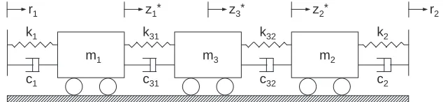
The entire structure — the emulated system — is represented by a hybrid numerical-experimental model where the dynamics of the numerical model are combined with the dynamics of the experimental component — the substructure. The general principle of substructuring remains the same regardless of the number of transfer systems present in the system, however the problem from a control point of view becomes more complicated for more than a single transfer system due to the intro-duction of cross-coupling between the control signals. In this paper, we will consider the example of a three mass oscillator system with two diametrically opposing exci-tation walls as shown in Figure 1. This will allow us to demonstrate the problems of achieving accurate control for multi-actuator substructuring using a conceptually simple example. This example has been discussed in detail by Wallaceet al.(2004), but for completeness will be briefly described here also. The masses are coupled by four identical linear springs,ki, and damped by coupled viscous dampers,ci, where i= 1,2,31,32. The system is excited via two moving supports,rj, wherej = 1,2.
The general equation of motion for such a system can be written as,
Mξ¨+Dξ˙+Kξ=Sr(t), (2.1) where, M, D and K are the mass, damping and stiffness matrices respectively and
Sr(t) is the support excitation. ξ is a vector which represents the states of the system, such that
ξ= [z∗
1, z2∗, z3∗] T
, (2.2)
where, (.)∗ is used to indicated that these dynamics are based on the ‘perfect’ dy-namics of the emulated system. In order to create a substructured model of the system shown in Figure 1, the middle mass, m3, and accompanying springs,k31
and k32, are taken to be the substructure. This leaves both excitation walls and
m1 k1
c1
z1*
r1
m3 k31
c31
z3*
xxxxxxxxxxxxxxxxxxxxxxxxxxxxxxxxxxxxxxxxxxxxxxxxxxxxxxxxxxxxxxxxxxxxxxxxxxxxxxxxxxxxxxxxxxxxxxxxxxxxxxxxxxxxxxxxxxxxxxxxxxxxxxxxxxxxxxxxxxxxxxxx xxxxxxxxxxxxxxxxxxxxxxxxxxxxxxxxxxxxxxxxxxxxxxxxxxxxxxxxxxxxxxxxxxxxxxxxxxxxxxxxxxxxxxxxxxxxxxxxxxxxxxxxxxxxxxxxxxxxxxxxxxxxxxxxxxxxxxxxxxxxxxxx xxxxxxxxxxxxxxxxxxxxxxxxxxxxxxxxxxxxxxxxxxxxxxxxxxxxxxxxxxxxxxxxxxxxxxxxxxxxxxxxxxxxxxxxxxxxxxxxxxxxxxxxxxxxxxxxxxxxxxxxxxxxxxxxxxxxxxxxxxxxxxxx xxxxxxxxxxxxxxxxxxxxxxxxxxxxxxxxxxxxxxxxxxxxxxxxxxxxxxxxxxxxxxxxxxxxxxxxxxxxxxxxxxxxxxxxxxxxxxxxxxxxxxxxxxxxxxxxxxxxxxxxxxxxxxxxxxxxxxxxxxxxxxxx
m2 k32
c32
z2*
k2
c2
[image:4.595.136.453.550.623.2]r2
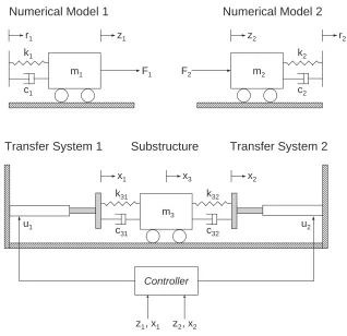
x1 m3 k31 c31 x3 k32 c32 x2
Numerical Model 1
Transfer System 1
F1 m1 k1 c1 z1 r1 xxxxxxxxxxxxxxxxxxxxxxxxxxxxxxxxxxxxxxxxxxxxxxxxxxxxxxxxxx xxxxxxxxxxxxxxxxxxxxxxxxxxxxxxxxxxxxxxxxxxxxxxxxxxxxxxxxxx xxxxxxxxxxxxxxxxxxxxxxxxxxxxxxxxxxxxxxxxxxxxxxxxxxxxxxxxxx m2 z2 k2 c2 r2 F2
Numerical Model 2
xxxxxxxxxxxxxxxxxxxxxxxxxxxxxxxxxxxxxxxxxxxxxxxxxxxxxxxxxx xxxxxxxxxxxxxxxxxxxxxxxxxxxxxxxxxxxxxxxxxxxxxxxxxxxxxxxxxx xxxxxxxxxxxxxxxxxxxxxxxxxxxxxxxxxxxxxxxxxxxxxxxxxxxxxxxxxx
Substructure
Transfer System 2
Controller
u2 u1
[image:5.595.135.453.84.392.2]z1, x1 z2, x2 xxx xxx xxx xxx xxx xxx xxx xxx xxx xxx xxx xxx xxx xxx xxx xxx xxx xxx xxx xxx xxx xxx xxx xxx xxx xxx xxx xxx xxx xxx xxx xxx xxx xxx xxx xxx xxx xxx xxx xxx xxxxxxxxxxxxxxxxxxxxxxxxxxxxxxxxxxxxxxxxxxxxxxxxxxxxxxxxxxxxxxxxxxxxxxxxxxxxxxxxxxxxxxxxxxxxxxxxxxxxxxxxxxxxxxxxxxxxxxxxxxxxxxxxxxxxxxxxxxxxxxxx xxxxxxxxxxxxxxxxxxxxxxxxxxxxxxxxxxxxxxxxxxxxxxxxxxxxxxxxxxxxxxxxxxxxxxxxxxxxxxxxxxxxxxxxxxxxxxxxxxxxxxxxxxxxxxxxxxxxxxxxxxxxxxxxxxxxxxxxxxxxxxxx xxxxxxxxxxxxxxxxxxxxxxxxxxxxxxxxxxxxxxxxxxxxxxxxxxxxxxxxxxxxxxxxxxxxxxxxxxxxxxxxxxxxxxxxxxxxxxxxxxxxxxxxxxxxxxxxxxxxxxxxxxxxxxxxxxxxxxxxxxxxxxxx xxxxxxxxxxxxxxxxxxxxxxxxxxxxxxxxxxxxxxxxxxxxxxxxxxxxxxxxxxxxxxxxxxxxxxxxxxxxxxxxxxxxxxxxxxxxxxxxxxxxxxxxxxxxxxxxxxxxxxxxxxxxxxxxxxxxxxxxxxxxxxxx xxxx xxxx xxxx xxxx xxxx xxxx xxxx xxxx xxxx xxxx xxxx xxxx xxxx xxxx xxxx xxxx xxxx xxxx xxxx xxxx xxxx xxxx xxxx xxxx xxxx xxxx xxxx xxxx xxxx xxxx xxxx xxxx xxxx xxxx xxxx xxxx xxxx xxxx xxxx xxxx
Figure 2. Schematic representation of asubstructured three mass system with two transfer systems
adjacent masses to be used to create two independent numerical models who’s in-fluence is imposed on the substructure by two separate transfer systems (actuators) via two independent control signals,u1 andu2. The influence of the substructure
is represented by two autonomous forces,F1 and F2, which are measured
experi-mentally and then imposed back on the numerical models. This new substructured model is shown schematically in Figure 2.
From Figure 2, the dynamics of the two numerical models can be written as,
m1¨z1+c1( ˙z1−r˙1) +k1(z1−r1) =F1,
m2¨z1+c2( ˙r2−z˙2) +k2(r2−z2) =F2. (2.3)
Due to the linear nature of the example considered here, we know explicitly the forces at each time interval allowing us to measure the accuracy of an individual test, where
F1=c31( ˙z3−z˙1) +k31(z3−z1),
F2=c32( ˙z2−z˙3) +k32(z2−z3). (2.4)
be measured using load cells between the transfer systems and the experimental substructure. This point highlights the difficulty in assessing the accuracy of sub-structuring tests for complex systems, as the end results of the test can never be compared with results from the emulated system. This point will be discussed in greater depth later in this section and in Section 2(f).
The aim of the control algorithm is to achieve synchronisation between the
desired interface displacement of the numerical models,z, and theactual position of the transfer systems,x. However, under just the linear control of the propriety controller, a transfer system will always be subject to some form of delay,τ,which can either be characterized as a pure delay or as a frequency dependent delay (lag) depending on the type of actuator. This error will lead to a reduction in the degree of synchronisation of the transfer system and thus a corresponding reduction in the accuracy of the numerical model compared to that of the emulated system (Mosqueda 2003). In fact the nature of this delay error in the substructuring model can be represented by two coupled components which we can write as,
e=e1(z∗, z, t) + e2(z, x, t), (2.5)
where,e1is a function which describes the accuracy of the numerical models
com-pared to the appropriate variable in the complete emulated system,
e1= [(z∗1−z1) (z2∗−z2)]T, (2.6)
ande2 represents the degree of synchronisation between each transfer system and
its numerical model (the local measure of accuracy for the control algorithm),
e2= [(z1−x1) (z2−x2)]T. (2.7)
Therefore, by combininge1ande2we can get a global measure of the accuracy of the
substructuring test which relates the emulated system coordinatesz∗to the actual displacement of the transfer systems x. However, when substructuring complex systems it is not possible to computez∗, and the only measure of accuracy is the degree of synchronisation e2. We note also that the numerical model coordinates
z are, in effect, a function of the transfer system x, as the force vector F will be subjected to the same delayτ as the transfer system, such that
z=f(r(t), F(t−τ)), (2.8) This highlights the nature of the coupling between e1 and e2. In the ideal case,
achieving perfect synchronisation by removing the delayτfrom the transfer systems will result ine2→0. This in turn will mean that the correct force vectorF(t) will
be added into the numerical models at the correct time, such that e1 → 0 and
the substructured system will replicate the dynamics of the emulated system. This argument allows us to propose the following:
Proposition 2.1. If the synchronisation error, e2= 0, for all timet≥0 during a
substructuring test thenx=zande1= 0such that the substructured model exactly
replicates the dynamics of the emulated system.
However, in practise the synchronisation error,e2, can never be exactly equal to
that ase2→0 the substructured model more closely replicates the dynamics of the
emulated system. The significance of Proposition 2.1 is that it gives an indication of the accuracy of a substructured system using the only measurable quantity of errore2, the local control error.
From an accuracy standpoint alone it is clear that the primary control objective should be to minimize e2, however the size of the delay τ also has a significant
effect on the stability of the substructuring algorithm as a whole. Any error ine2
will result in a corresponding error ine1 and thus propagate to the next time step
leading to potential instability of the substructuring algorithm. This is discussed further in Section 2(b).
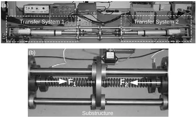
(a) Experimental setup
To implement substructuring we are using a combination of standard Simulink blocks and custom S-Functions (C modules compiled into *.dll files using a MEX compiler) to formulate a model and a dSpace DS1104 R&D Controller Board to implement it in real-time. The companion software ControlDesk is used for online analysis and control, providing soft real-time access to the hard real-time applica-tion. More detail on the experimental setup is given by Wallaceet al.(2004).
Figure 3 (a) shows the substructured model setup along with the transfer sys-tems which imposes the interface displacements on the physical substructure. An expanded view is shown in Figure 3(b). Each mass is a constant 2.2kg and connected via three parallel shafts constraining their motion to one degree of freedom. Through system identification the springs were found to have a stiffness ofk = 9000N/m and damping value ofc = 30Ns/m. The stiffness of the strings allows significant coupling between the two transfer system, this is discussed further in Section 3(f).
(a)
(b)
Transfer System 1 Transfer System 2
Substructure
F
1F
2 [image:7.595.123.450.416.614.2](b) Effect of feedback delay on the substructuring algorithm
There is an important difference between the difficulties faced in a standard control problem to that faced when performing substructuring. For substructuring, the reference signal (i.e. the control demand) for each transfer system is not known at the start of each time step as in a normal control problem, but must be created in its respective numerical model during each time period. A small delay in the transfer system response (such thate26= 0, from Equation 2.7) introduces a corresponding
error in the feedback force vector, which can be thought of as adding negative damping to the system (Horiuchi et al. 1999). This discrepancy has the effect of reducing the accuracy of the numerical models (compared to the emulated system) until the magnitude of the synchronisation delay increases to such a degree that a sign change for the damping of the overall system occurs. At this point instability of the substructuring algorithm is observed and is be characterized by the onset of oscillations with exponential growth (Wallaceet al.2004).
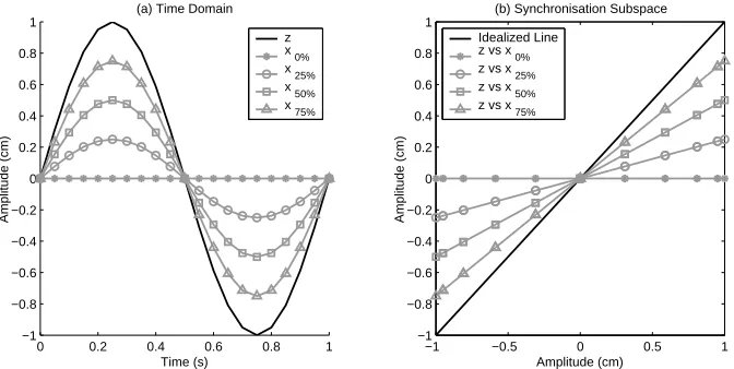
(c) Measuring synchronisation accuracy using subspace plots
Synchronisation subspace plots are used to show the effectiveness of the con-trol algorithm by plotting the desired verses actual responses, (Ashwin 1998). A subspace plot shows the amplitude accuracy and the magnitude of delay coupled together at any one time interval. Perfect synchronisation is represented by a diag-onal straight line with maxima and minima of the reference signal. Any reduction in synchronisation can be seen as a deviation from this idealized line. For periodic wall excitation conditions these plots build up into a repeating periodic pattern, which can appear complex. However, the individual components of amplitude and delay produce their own specific and identifiable patterns if evaluated separately.
The result of varying the amplitude accuracy is to change the angular orienta-tion of the subspace plot compared to the idealized line. Figure 4 shows the result of increasing amplitude accuracy from a 0% to 25%, 50% and then 75% of perfect synchronisation. Continuing this trend, the angular orientation further increases to
0 0.2 0.4 0.6 0.8 1 −1
−0.8 −0.6 −0.4 −0.2 0 0.2 0.4 0.6 0.8 1
(a) Time Domain
Time (s)
Amplitude (cm)
−1 −0.5 0 0.5 1 −1
−0.8 −0.6 −0.4 −0.2 0 0.2 0.4 0.6 0.8 1
(b) Synchronisation Subspace
Amplitude (cm)
Amplitude (cm)
z x
0%
x
25%
x
50%
x 75%
Idealized Line z vs x
0%
z vs x
25%
z vs x
50%
z vs x 75%
[image:8.595.118.454.458.627.2]1 1.2 1.4 1.6 1.8 2 −1
−0.8 −0.6 −0.4 −0.2 0 0.2 0.4 0.6 0.8 1
(a) Time Domain
Time (s)
Amplitude (cm)
−1 −0.5 0 0.5 1 −1
−0.8 −0.6 −0.4 −0.2 0 0.2 0.4 0.6 0.8 1
(b) Synchronisation Subspace
Amplitude (cm)
Amplitude (cm)
Idealized Line z vs xτ
1
z vs xτ
2
z vs xτ3 z
xτ
1
xτ
2
xτ3
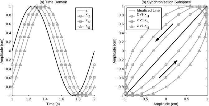
Figure 5. Effect of increasing delay with perfect amplitude accuracy.
a limit of a 90◦ (vertical) line which is the outcome of an infinite plant response. The consequence of introducing a constant delay between the reference signal and the plant response is to transform the idealized straight line into an ellipse (anti-clockwise implies negative damping, (anti-clockwise implies positive damping) as shown by Figure 5(b). The greater the delay, the larger the width of the minor axis of the ellipse, with the change being proportional to the delay magnitude. If the delay is not constant through one period, then the ellipse no longer has a uniform shape.
In a typical subspace plot however, the effect of amplitude and delay are coupled together with both being able to vary independently through a single period. How-ever, despite this, their visual interpretation remains simple instant online guide to the accuracy of an individual test, thus allowing linear controllers to be tuned online and adaption characteristics to be viewed. This technique will allow us to measure the effectiveness of the forward prediction algorithms presented in Section 3.
3. Forward prediction
(a) Application to forward prediction
The value of being able to forward predict online can be seen from Figure 6. Controlling to an arbitrary reference signal z we see that there is an inevitable delayτin the dynamic response of the plantx(expected in any dynamical system under linear control). By predicting forward the same amount as the delay τ to create a new reference signalz′, at any point in timetn, and then using this new reference as the transfer system demand, we will be able to eliminate the response delay thus obtaining nominally zero synchronisation error, such thate2 →0 from
Equation 2.7.
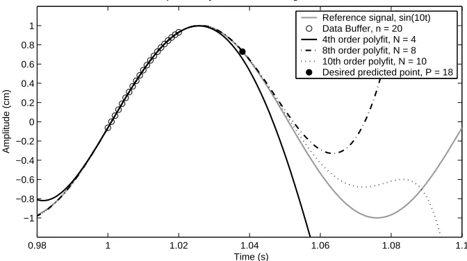
Figure 7 shows an example sinusoid reference signal of 10Hz (shown by the solid grey line) which is to be predicted forward. A section of data must be taken to act as control points for the fitted polynomial curve, here a buffer of 20 data points
[image:9.595.119.455.87.257.2]0 0.1 0.2 0.3 0.4 0.5 0.6 0.7 0.8 0.9 1 −1
−0.8 −0.6 −0.4 −0.2 0 0.2 0.4 0.6 0.8 1
Time (s)
Amplitude (cm)
z’ z x
τ ∆tP
t
n
e
[image:10.595.118.454.87.266.2]2→ 0
Figure 6. Delay compensation for transfer system dynamics by creating a forward predicted signalz′.
in this case) Figure 7 shows the differing accuracies obtained by the various order
N of polynomial fitted curves. From this example, we see that both the 8th and 10th order curves have the highest degree of accuracy, whereas the 4th order curve loses coherence much more quickly. However, the higher the order of prediction the more computationally intensive the calculation and the more inherently unstable the predicted signalz′will become. Therefore, the desired amount of time for which the numerical model should be predicted forward is equal to τ =△tP to achieve optimal delay compensation.
0.98 1 1.02 1.04 1.06 1.08 1.1
−1 −0.8 −0.6 −0.4 −0.2 0 0.2 0.4 0.6 0.8 1
Time (s)
Amplitude (cm)
Least Squares Polynomial Curve Fitting of Buffered Data
Reference signal, sin(10t) Data Buffer, n = 20 4th order polyfit, N = 4 8th order polyfit, N = 8 10th order polyfit, N = 10 Desired predicted point, P = 18
[image:10.595.116.452.438.626.2](b) Least squares polynomial fitting
One mathematical procedure for finding the best fitting curve to a given set of points is by minimising the sum of the squares of the offsets of the points from the curve (Kreyszig 1999). The linear least squares fitting technique is the simplest and most commonly applied form of linear regression and provides a solution to the problem of finding the best fitting straight line through a set of points. However, due to the dynamics of the numerical models in our system we move from a best-fit line to a best-fit polynomial, where sums of vertical distances are used. A polynomial inxof orderN with coefficientsai (wherei= 0, . . . , N) is given by,
y=a0+a1x+. . .+aNxN. (3.1)
Using a standard least squares polynomial derivation (Kreyszig 1999), givenn num-ber of data points (x0, y0), . . . ,(xn−1, yn−1) with polynomial coefficientsa0, . . . , aN
the equation of the curve is given by,
y0
y1
.. .
yn−1
=
1 x0 x20 . . . xN0
1 x1 x21 . . . xN1
..
. ... . .. ...
1 xn−1 x2n−1 . . . xNn−1
a0
a1
.. .
aN
. (3.2)
Therefore, in matrix notation, the equation for a polynomial fit is given by
y=Xa, (3.3)
which can be solved by premultiplying by the matrix transpose, such thatXTy=
XTXa. The matrix can then be inverted directly to give the solution,
a= (XTX)−1XT
y. (3.4)
(c) Single time step forward prediction
Delay compensation by polynomial extrapolation is not a new concept, single time step prediction techniques have already been proposed in relation to substruc-turing (Horiuchiet al.1999; Darbyet al. 2001a), and shown to improve accuracy. These algorithms are based on using predefined coefficients, ¯ai, for an Nth order
polynomial fit ofnnumber of control points following the equation,
z′ =
N X
i=0
¯
ai zi, (3.5)
where z0 is the present calculated numerical model displacement and zi are the
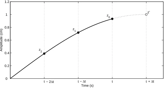
previously calculated displacements at ∆t×iunits of time ago. Figure 8 shows the forward predicted pointz′being obtained by extrapolating the polynomial function over the present displacement z0 and N previous calculated values, thus making
the number of control points used,n= (N+ 1).
For this 2nd order polynomial fit we attain the following constants ¯a 0 = 3,
¯
a1 = −3 and ¯a2 = 1 (Horiuchi et al. 1999). Note that we can only predict one
t t t t 0
0.2 0.4 0.6 0.8 1 1.2
Time (s)
Amplitude (cm)
− 2∆t − ∆t + ∆t
z
0
z
1
z
2
[image:12.595.118.454.86.266.2]z’
Figure 8. Single time step prediction ofn= 3 control points for aN= 2 order polynomial fit.
the polynomial function (to ensure that theX matrix of Equation 3.3 is square) otherwise the polynomial fit will not hold. To predict further ahead than one time step we can simply apply Equation 3.5 more than once (Darbyet al. 2001a). For example to predict two time steps forward we see that if
z′(∆t)= 3
z0−3z1+z2, (3.6)
then,
z′(2∆t) = 3z′(∆t)−3z
0+z1,
= 6z0−8z1+ 3z2. (3.7)
Note that we are still restricted to predicting in whole time steps unless an addi-tional interpolation is carried out between the two points (Darbyet al.2001a).
However, if we use Equation 3.4 to solve the (XTX)−1XT matrix components
numerically first, we can deduce a more generalised forward prediction algorithm where multiples and fractions of one time step can be predicted in one iteration and we are no longer constrained to n= (N + 1) number of control points. Increasing
ncan help to smooth noise out of the numerical model and thus from the control signal. We define the size of the X matrix by choosing values for the number of control pointsnand the order of the polynomial fitN. For the case above,n= 3 andN = 2, thus rewriting the general Equation 3.3 for this specific case gives us,
z0
z1
z2
=
1 t0 t20
1 t1 t21
1 t2 t22
a0
a1
a2
, (3.8)
where,tiis the current simulation time for each value ofzi. Therefore, for a sample
time step size ∆t as shown in Figure 8,
z0
z1
z2
=
1 0 0
1 −∆t ∆t2
1 −2∆t 4∆t2
a0
a1
a2
The predicted pointz′ is given by an adaptation of Equation 3.3,
z′=X
P a, (3.10)
where,XP is the forward prediction vector and given by,
XP = [1 P∆t . . . PN∆tN], (3.11)
andPis the number of time steps to be predicted forward (which does not have to be a integer multiple of ∆t). AsXis a square matrix in this case, (XTX)−1XT =
X−1,
therefore,
z′=X
PX−1z. (3.12)
EvaluatingXPX−1 gives an expression which is independent of the sample time
step size ∆t. Substituting into Equation 3.12 for the case whenP = 1 we see that
z′(∆t)= 3z
0−3z1+z2, (3.13)
thus matching the coefficients of the one step method in Equation 3.6. Substituting
P= 2 we see that
z′(2∆t)= 6
z0−8z1+ 3z2, (3.14)
matching the coefficients found in Equation 3.7 but in a single operation. There-fore, the coefficients ¯ai from Equation 3.5 are actually the pre-multiplication of the
forward prediction vectorXP for the special case ofP = 1, such that
¯
a=XP[(XTX)−1XT]. (3.15)
In this way, the coefficients ¯aare predefined and thus fix the level of forward predic-tion obtained, whereas the coefficients of the polynomial funcpredic-tionaare calculated each time step and therefore allow variable degrees of forward prediction to be achieved by altering the value ofP online.
(d) Online forward prediction using variable polynomial coefficients
To achieve online forward prediction a buffer ofndata points of the numerical model displacementz are stored and updated by a buffer overlap of (n−1) each time step. These are then fed into a least squares polynomial fitting sub routine which uses the set of control points [zn−1, zn−2, . . . , z0] to calculate theNthorder
polynomial fit and therefore find the coefficient vectorafrom Equation 3.4 for that time step. The current coefficients are then fed into a reconstruction algorithm that calculates the predicted pointz′according to Equation 3.10 using the forward prediction vectorXP, such that
z′=ka
N X
i=0
(aiPN). (3.16)
(e) Adaptive forward prediction (AFP)
The basic forward prediction algorithm can be used to effectively remove the transfer system delay, however, both the magnitude of the forward prediction,P, and the amplitude gain,ka, must be specifically tuned for each different excitation
condition, thus making the algorithm, in effect, a feed-forward controller. To remove the need for this tuning and to allow the algorithm to achieve high levels of syn-chronisation for frequency dependent and transient plant conditions we must close the control loop and use the feedback dynamics of the transfer system. In com-bination with the existing linear control present in the substructuring algorithm this model structure now represents an error driven adaptive feedback controller (˚Astr¨om & Wittenmark 1995). We cannot explicitly measure the transfer system delay τ as we only have data for the current time step, thus we only know the synchronisation errore2at any single point in time. Therefore, to achieve complete
delay compensation we can indirectly force τ → 0 by explicitly using a measure of the synchronisation errore2. An alternative technique which uses this feedback
error to achieve adaptive compensation is presented by Darbyet al.(2002). As before, the current coefficients are fed into a reconstruction algorithm that calculates the predicted pointz′ but now the magnitude of the forward prediction
τ is now governed by,
τ= ∆t(P+ρ), (3.17) where, ∆t is the sample time step size,P is thefixed initial number of time steps to be forward predicted andρis the adaptive number of time steps to be forward predicted. Likewise, the amplitude accuracy is now governed by,
z′=z′(k
a+σ), (3.18)
where,kais thefixed amplitude gain andσis anadaptive amplitude variable which
together control the amount of the predicted reference signal to be used.
Setting P = 0 and ka = 1 will bring about zero initial conditions. The delay
compensation can then be completely achieved by the adaptive parameter ρ and the amplitude error completely removed byσ. Thus, we can use this new adaptive algorithm when we have no knowledge of the plant dynamics and when there is transient or frequency dependent plant behaviour. However, it is not always de-sirable to start from zero initial conditions, in fact in many cases (and mainly in earthquake engineering) it is important to start the test with the AFP algorithm in a state near to optimal adaptation. These optimal values can be estimated by ob-serving the steady state adaptive values of an uncoupled system identification test for the specific transfer system. This would then allow the initial transient phase of the test to be avoided.
The adaption algorithm works off four triggered states,ϕ1,...,4, which have a null
value until their individual trigger conditions are met. Trigger states, ϕ1 and ϕ2,
are activated on the condition of sign change of the numerical model displacement, when z has zero amplitude. The first state represents a rising edge, z changing from negative to positive, and the second a falling edge,zchanging from positive to negative. The other two trigger states are similar except activated on the condition of sign change of the numerical model velocity, ˙z, withϕ3representing a rising edge
andϕ4representing a falling edge. Effectively these two conditions give the time at
The adaptive forward prediction parameter ρis calculated when either of the first two triggered statesϕ1,2are met. This allows the delay of the transfer system
response to be observed independently from any amplitude error. The value ofρis given by,
ρn+1=ρn ± αe
γ
2,n , (3.19)
where, α is an adaptive gain parameter for the magnitude of forward prediction and γ sets the convergence curve and must be greater than or equal to 1. Note that the±relates to whether the signal is a rising or falling edge. Equation 3.19 shows that when the synchronisation errore2 is zero,ρn+1=ρn thusρretains its
previous value, indicating that full delay compensationτ has been achieved. Similarly, the adaptive amplitude parameter is calculated when either of the second two triggered states ϕ3,4 are met. This allows the peak of the numerical
model to be compared to that of the transfer system once delay compensation has occurred. The value ofσis given by,
σn+1=σn ± βeγ2,n, (3.20)
where,β is an adaptive gain parameter for the amplitude accuracy. Note that until full delay compensation has been achieved the parameter σ will give an under estimation of the amplitude error. However, as the delay is by far the dominant factor in the compensation algorithm this condition does not effect the performance of the controller.
We see that by setting both adaptive parametersαandβ to zero, the adaption algorithm can be turned ‘off’ resulting in the basic feed-forward controller, assum-ing both ρ0 and σ0 equal zero. Note that both Equations 3.19 and 3.20 include
history data, analogous to that of an integrator, such that any steady state error is forced to zero. The choice ofγdecides the convergence curve. The synchronisation error should be such that e2 << 1 so the higher γ, the slower the convergence
at very low instances of synchronisation error, thus the smoother the steady state values for the adaptive parameters but the less reactive it is to fast transient or frequency dependent plant behaviour. Additionally, as the adaption only occurs at the set trigger conditions,ϕ1,...,4, the AFP algorithm is subject to a persistence of
excitation criterion (˚Astr¨om & Wittenmark 1995).
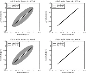
(f) Substructuring using the AFP algorithm
To show the effectiveness of the AFP algorithm, we first perform a substructur-ing test ussubstructur-ing forces generated by a model of theemulated system, rather than the actualmeasured forces as this will ensure that the numerical models will exactly match the dynamics of the emulated system, such thate1 = 0 from Equation 2.6.
−1.5 −1 −0.5 0 0.5 1 1.5 −1.5
−1 −0.5 0 0.5 1 1.5
(a1) Transfer System 1 − AFP off
Amplitude (cm)
Amplitude (cm)
Idealized z
1* vs x1
−1.5 −1 −0.5 0 0.5 1 1.5 −1.5
−1 −0.5 0 0.5 1 1.5
(a2) Transfer System 1 − AFP on
Amplitude (cm)
Amplitude (cm)
Idealized z
1* vs x1
−1.5 −1 −0.5 0 0.5 1 1.5 −1.5
−1 −0.5 0 0.5 1 1.5
(b1) Transfer System 2 − AFP off
Amplitude (cm)
Amplitude (cm)
Idealized z2* vs x2
−1.5 −1 −0.5 0 0.5 1 1.5 −1.5
−1 −0.5 0 0.5 1 1.5
(b2) Transfer System 2 − AFP on
Amplitude (cm)
Amplitude (cm)
[image:16.595.135.437.86.344.2]Idealized z2* vs x2
Figure 9. Synchronisation subplots for equal and opposite wall sweep excitation ofr1,2= 3
to 10Hz in 5s and then back to 3Hz in 5s. Controller parametersN= 4,n= 10,α1,2 = 100,
β1,2= 5,γ1,2= 2; Adaptive parameters shown in Figure 10.
(a2) and (b2). It is clear that the use of the AFP algorithm results in a significant improvement in the level of synchronisation. The constantly changing conditions means that the delay compensation scheme never reaches steady state values but in-stead must constantly monitor the synchronisation error in order to maintain a high
0 2 4 6 8 10
9.5 10 10.5 11 11.5
(a) Delay Compensation Adaption Characteristics
Time (s)
Adaptive Forward Prediction (P = 0 ms)
ρ1 ρ2
0 2 4 6 8 10
0.85 0.9 0.95 1 1.05 1.1
(b) Amplitude Error Adaption Characteristics
Time (s)
Adaptive Amplitude Correction (k
a
= 1) ρρ1
2
[image:16.595.117.455.474.626.2]level of compensation. Although the excitation demands are equal and opposite and the actuators are of the same type, we can see that the transfer system dynamics vary as shown by the differing adaption characteristics in Figure 10 (a). This is a marked difference to the similarity of the amplitude error shown in Figure 10 (b). This highlights the need for the control of the transfer systems to be decoupled such that their specific mechanical characteristics can be dealt with independently. However, to achieve a true real-time dynamic substructuring test the actual
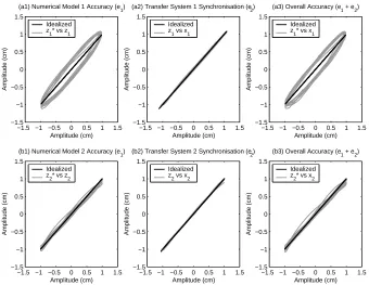
force must be fed back into its respective numerical model rather than the one gen-erated by a model of theemulated system. Figure 11 shows the steady state results for both transfer systems for such a test using the AFP algorithm. Firstly, it can be seen that the substructuring algorithm has remained stable due to the high degree of synchronisation between the numerical models and their respective transfer sys-tems, shown by Figure 11 (a2) for Transfer System 1 and (b2) for Transfer System 2. In both cases, virtually all the delay has been removed. The resulting numerical models can then be compared to their respective emulated dynamics — shown in Figures 11 (a1) and (b2). The reduction in synchronisation of the numerical models highlights the fact that although thelocal control error is small a sizeable substruc-turing error exists. The reason for the extent of the substrucsubstruc-turing error in this case is the magnitude of cross coupling between the transfer systems. Figure 12 shows the manufacture’s specification for the actuator capacity envelope for the transfer systems used in these experiments. The experimental data shown is for Transfer
−1.5 −1 −0.5 0 0.5 1 1.5 −1.5 −1 −0.5 0 0.5 1 1.5
(a1) Numerical Model 1 Accuracy (e
1)
Amplitude (cm)
Amplitude (cm)
−1.5 −1 −0.5 0 0.5 1 1.5 −1.5 −1 −0.5 0 0.5 1 1.5
(a2) Transfer System 1 Synchronisation (e
2)
Amplitude (cm)
Amplitude (cm)
−1.5 −1 −0.5 0 0.5 1 1.5 −1.5 −1 −0.5 0 0.5 1 1.5
(a3) Overall Accuracy (e
1 + e2)
Amplitude (cm)
Amplitude (cm)
−1.5 −1 −0.5 0 0.5 1 1.5 −1.5 −1 −0.5 0 0.5 1 1.5
(b1) Numerical Model 2 Accuracy (e
1)
Amplitude (cm)
Amplitude (cm)
−1.5 −1 −0.5 0 0.5 1 1.5 −1.5 −1 −0.5 0 0.5 1 1.5
(b2) Transfer System 2 Synchronisation (e
2)
Amplitude (cm)
Amplitude (cm)
−1.5 −1 −0.5 0 0.5 1 1.5 −1.5 −1 −0.5 0 0.5 1 1.5
(b3) Overall Accuracy (e
1 + e2)
Amplitude (cm)
Amplitude (cm)
Idealized z
1* vs z1
Idealized z
1 vs x1
Idealized z
1* vs x1
Idealized z
2* vs z2
Idealized z
2 vs x2
Idealized z
[image:17.595.118.458.343.606.2]2* vs x2
Figure 11. Comparative synchronisation subplots for a real substructuring test for wall excitation ofr1,2 = 8Hz(excitation magnitudes are not equal) using the AFP algorithm;
¯
0 100 200 300 400 500 600 700 0
50 100 150 200 250 300 350 400 450
Force (N)
Velocity (mm/s)
[image:18.595.134.434.86.257.2]Manufacturer specification Experimental profile (modulus)
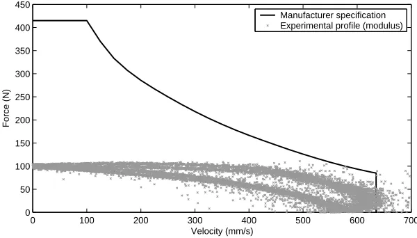
Figure 12. Actuator capacity envelope for Transfer System 1. Experimental data shown for the test of Figure 11(a) (10s test data).
System 1 (although a similar profile would be observed for Transfer System 2) for the test shown in Figure 11(a). It is typical in real-time substructuring that the actuators are operated right up to their maximum performance envelope. It is close to and beyond this envelope that the cross-coupling and other nonlinear effects become significant. However despite this, good local synchronisation is maintained by the AFP algorithm.
Figure 13 shows the case where the AFP algorithm is not used, such that the delay experienced due to a standard linear controller is not removed. The substruc-turing test is started using the emulated force vector to ensure stability and then switched over to theactual force vector after approximately 3 seconds of run time. We observe the instability of the substructuring algorithm immediately building in Figure 13 (a). It is important to note that it is not the controller which is becoming unstable as can be seen from Figure 13 (b), which shows a consistent transfer system
2.6 2.8 3 3.2 3.4 3.6 3.8
−2 −1.5 −1 −0.5 0 0.5 1 1.5 2
(a) Destabilization of the Substructuring Algorithm
Time (s)
Amplitude (cm)
−2 −1 0 1 2
−2 −1.5 −1 −0.5 0 0.5 1 1.5 2
Amplitude (cm)
Amplitude (cm)
(b) Transfer System Synchronisation
z
1*
z
1
Idealized z
1 vs x1
AFP off
[image:18.595.117.452.480.618.2]7 7.05 7.1 7.15 7.2 7.25 7.3 −0.4
−0.3 −0.2 −0.1 0 0.1 0.2 0.3 0.4
Time (s)
Amplitude (cm)
(a) Time Domain Response
−0.4 −0.2 0 0.2 0.4 −0.4
−0.3 −0.2 −0.1 0 0.1 0.2 0.3 0.4
Amplitude (cm)
Amplitude (cm)
(b) Synchronisation Subspace
z
3*
x
3
[image:19.595.118.458.86.225.2]Idealized z3* vs x3
Figure 14. Accuracy of the substructure dynamics for the test of Figure 11.
delay throughout the entirety of the test. This example shows that the removal of the transfer system delay is essential in ensuring a stable substructuring algorithm (Horiuchiet al.1999).
The overall resultingglobal accuracy of the substructuring test using the AFP algorithm is shown in Figures 11 (a3) and (b3), which indicates the level of synchro-nisation between the emulated system and the resulting transfer system dynamics. As stated in Equation 2.5, the global error is a linear addition of the two sources of error,e1ande2. However, we note thate1often cannot be calculated when
perform-ing a complex substructurperform-ing test as the emulated dynamics would not be known explicitly. Figure 14 shows the result of the global error in the dynamics of the sub-structurex3compared to that of the emulated systemz3∗for the example presented
in Figure 11. The combination of the local control error and the numerical model error due to the cross coupling of the transfer systems has resulted in a non-linear relationship of the substructure dynamics compared to that of the emulated system. This is an important concept for measuring the accuracy of a substructuring test as the only error that we have a direct influence on is the level of synchronisation achieved,e2. The magnitude of the numerical model error,e1and thus the resulting
global error is dependent on the capacity of the transfer systems used to perform the test. Working well within the actuator’s performance envelope will result in limited coupling between the transfer systems and therefore a correspondingly lower global error. For a complex substructured system this means that the explicit measure of accuracy,e2 (the local control error), needs to be assessed in combination with the
experimental transfer system profile (compared to its actual performance envelope) to gain a more complete measure of the accuracy of a substructuring test.
4. Conclusions
described, using synchronisation theory, how these delay errors can be measured. We have described a measure of the accuracy of the substructuring algorithm without having to simulate the complete system. This is a generic result which holds for all substructured systems, although the exact relationship betweene1 ande2 will be
system dependant.
In Section 3(d) we have shown how the resulting delay errors can be removed by using an online forward prediction technique. This is based on a polynomial es-timation to compensate for the delay present in the transfer systems. In addition to accuracy, this technique has benefits in achieving a stable substructuring algorithm. In Section 3(c) the algorithm presented here is compared with existing techniques and shown to be a more generic approach than the single step algorithms applied to substructuring thus far. This gives considerable advantages in terms of flexibility and accuracy.
Finally in Section 3(e) we have shown how the basic forward prediction algo-rithm can be extend to one with adaption by closing the control loop to achieve an error driven adaptive feedback controller. This allows the forward prediction algorithm to accurately cope with frequency dependent plant behaviour and oper-ate with no prior knowledge of the plant characteristics. We show that the AFP algorithm can be used to achieve a stable substructuring algorithm despite the discrepancies in the dynamics of the numerical models compared to those of the emulated system. This is in contrast to the immediate exponential growth observed when the test is carried out using a standard linear controller in isolation.
Acknowledgements
Two authors would like to acknowledge the support of the EPSRC: Max Wallace is supported via an EPSRC DTA and David Wagg via an EPSRC Advanced Research Fellowship.
References
˚
Astr¨om, K.J. & Wittenmark, B. 1995Adaptive Control, Addison Wesley.
Ashwin, P. 1998 Non-linear dynamics, loss of synchronisation and symmetry breaking, Proc. of the Institution of Mech. Engrs, Part G,212(3), 183–187.
Blakeborough, A., Williams, M.S., Darby, A.P. & Williams, D.M. 2001The development of real-time substructure testing, Phil. Trans. R. Soc. Lond., Series A,359, 1869–1891. Darby, A.P., Blakeborough, A. & Williams, M.S. 2001a Improved control algorithm for
real-time substructure testing, Earthquake Engng Struct. Dyn.,30, 431–448.
Darby, A.P., Blakeborough, A. & Williams, M.S. 2001bReal-time substructure tests using hydraulic actuator, J. Engng Mech., Amer. Soc. Civ. Engrs,125(10), 1133–1139. Darby, A.P., Williams, M.S. & Blakeborough, A. 2002Stability and delay compensation
for real-time substructure testing, J. Engng Mech., Amer. Soc. Civ. Engrs, 128(12), 1276-1284.
Donea, J., Magonette, P., Negro, P., Pegon, P., Pinto, A. & Verzeletti, G. (1996) Pseudo-dynamic capabilities of the ELSA laboratory for earthquake testing of large structures, Earthquake Spectra,12(1), 163–180.
Horiuchi, T., Inoue, M., Konno, T. & Namita, Y. 1999 Real-time hybrid experimental system with actuator delay compensation and its application to a piping system with energy absorber, Earthquake Engng Struct. Dyn.,28, 1121–1141.
Kreyszig, E. 1999Advanced Engineering Mathematics, 8th Edition, New York: Wiley. Mahin, S.A. & Shing, P.B. 1985Pseudodynamic method of seismic testing, J. Strut. Engng,
111, 1482–1503.
Mosqueda, G. 2003 Continuous hybrid simulation with geographically distributed sub-structures. Ph.D. thesis, University of California, Berkeley.
Nakashima, M., Kato, H. & Takaoka, E. 1992Development of real-time pseudo dynamic testing, Earthquake Engng Struct. Dyn.,21, 779–792.
Nakashima, M. & Masaoka, N. 1999Real-time on-line test for MDOF systems, Earthquake Engng Struct. Dyn.,28(4), 393–420.
Neild, S.A., Drury, D., Wagg, D.J., Stoten, D.P. & Crewe, A.J. Implementing real time adaptive control methods for substructuring of large structuresProc. of the 3rd World Conf. on Structural Control, Como, Italy, 7-12 April 2002, pp. 811–817.
Neild, S.A., Stoten, D.P., Drury, D. & Wagg, D.J. 2005 Control issues relating to real-time substructuring experiments using a shaking table, Earthquake Engng Struct. Dyn., 34(9), 1171–1192.
Pinto, A.V., Pegon, P., Magonette, G. & Tsionis, G. 2004 Pseudo-dynamic testing of bridges using non-linear substructuring, Earthquake Engng Struct. Dyn.,33(11), 1125– 1146.
Sivaselvan, M.V., Reinhorn, A., Liang, Z. and Shao, X. Real-time dynamic hybrid testing of structural systemsProc. of the 13th World Conf. Earthquake Engineering, Vancouver, Canada, 1-6 August, 2004, Paper No. 1644, pp. 1–14.
Wagg, D.J. & Stoten, D.P. 2001 Substructuring of dynamical systems via the adaptive minimal control synthesis algorithm, Earthquake Engng Struct. Dyn.,30, 865–877. Wallace, M.I., Wagg, D.J. & Neild, S.A. Multi-actuator substructure testing with
appli-cations to earthquake engineering: how do we assess accuracy?Proc. of the 13th World Conf. Earthquake Engineering, Vancouver, Canada, 1-6 August, 2004, Paper No. 3241, pp. 1–14.