White Rose Research Online
Universities of Leeds, Sheffield and York
http://eprints.whiterose.ac.uk/
This is an author produced version of a paper published in
Combustion Theory
and Modelling.
White Rose Research Online URL for this paper:
http://eprints.whiterose.ac.uk/3664/
Published paper
Sharpe, G.J. and Falle, S.A.E.G. (2006)
Nonlinear cellular instabilities of planar
premixed flames: numerical simulations of the Reactive Navier-Stokes equations.
Combustion Theory and Modelling, 10 (3). pp. 483-514.
flames: numerical simulations of the Reactive
Navier-Stokes equations.
G J Sharpe†and S A E G Falle‡
†School of Mechanical Engineering, University of Leeds, Leeds, LS2 9JT, UK
‡Department of Applied Mathematics, University of Leeds, Leeds, LS2 9JT, UK E-mail: [email protected]
1. Introduction
A premixed flame is a slow combustion wave which propagates via conduction of heat and diffusion of chemical species between the hot burnt products and the cold unburnt fuel. Premixed flames may propagate as planar and steady waves, but experiments show that in many cases the flame is actually wrinkled and possibly time-dependent (Buckmaster & Ludford 1982; Sivashinsky 1983; Strehlow 1985). These multi-dimensional flame fronts are known as ‘cellular’ flames. Cellular flames may be regarded as the outcome of thermal-diffusive and/or hydrodynamic instabilities of the underlying planar front. Hence a first step in understanding the origins of cellular flames is a linear stability analysis of steady, planar flames. Such analyses have been performed using the asymptotic limits of high activation energy and near-equidiffusional flames (NEFs) (Lewis numbers asymptotically close to unity), sometimes together with further simplifications such as the constant density model (CDM), which is formally valid in the limit of small heat release, or slowly varying flames (SVFs), where the wavelength of the perturbation is assumed to be much larger than the flame thickness (Sivashinsky 1977a; Frankel & Sivashinsky 1982; Matalon & Matkowsky 1982; Pelce & Clavin 1982; Jackson & Kapila 1984).
Denet & Haldenwang (1992) (for the CDM thermal-diffusive model) and Denet & Haldenwang (1995) and Kadowaki (1997,1999,2000) (for the full Reactive Navier-Stokes model) used numerical simulations in order to calculate initial (linear) growth rates for different disturbance wavelengths. For both the CDM and Navier-Stokes models, these authors found quantitative differences to the predictions of the asymptotic linear stability theories. However, as argued by Lasseigne, Jackson & Jameson (1999), using numerical simulations to determine linear growth rates or to validate the linear stability theories is not the correct philosophy. Instead, a major use of linear stability results should be in guiding and validating numerical schemes for simulating the full non-linear problem. Capturing the correct initial growth rates and stability boundaries, as predicted by the linear analysis, should be an essential test problem for numerical codes constructed to simulate flame problems (Lasseigne
et al. 1999). This philosophy has been used for some time in validating detonation simulations (e.g. Sharpe & Falle 2000a, b)
However, at the time the calculations of Denet & Haldenwang (1992,1995) and Kadowaki (1997,1999,2000) were performed, only high activation energy asymptotic linear stability results were available, but their numerical simulations by necessity employed finite but realistic activation energies since the reaction zone, which must be resolved in the simulations (Lasseigneet al. 1999, Sharpe 2003), becomes extremely thin as the activation energy increases and thus the simulations become difficult if the activation energy is too high. For such finite activation energies, the asymptotic results may give only qualitative results, and hence cannot be used for quantitative tests for numerical schemes. Instead, linear stability analyses using the same parameters, including finite activation energy, are required to determine the exact (i.e. not asymptotic) linear dispersion relations, which can then be used to validate numerical codes.
Finite activation energy linear stability results have been achieved more recently, by Lasseigne et al. (1999) for the CDM, by Liberman et al. (1994) for the purely hydrodynamic case (Lewis number of unity) and by Sharpe (2003) for the full Reactive Navier-Stokes model with arbitrary Lewis numbers. The works of Lasseigne et al.
thermal-diffusive effects have a major role in the cellular instability) unphysically high activation energies are required for the high activation energy asymptotics to give quantitatively accurate results. Thus for the moderate but realistic activation energies typically used in simulations, the asymptotic results give quantitatively poor predictions of growth rates and hence are inappropriate as test problems for Lewis numbers less than unity. Furthermore, Sharpe (2003) showed that additional CDM and SVF approximations do not give quantitative accurate predictions for any realistic parameter set, even at large activation energies.
Lasseigne et al. (1999) used their linear stability results very effectively to validate their numerical code and hence to show that the discrepancies between the stability boundaries found from simulations of Rogg (1982) and the linear stability prediction was due entirely to Rogg’s simulations not resolving the reaction zone at large activation energies. Sharpe (2003) used his linear results to resolve discrepancies between the results of simulations by Fr¨olich & Peyret (1991) and those by Denet & Haldenwang (1995), in that it was shown Fr¨olich & Peyret’s (1991) algorithm failed to obtain the correct results at higher activation energies. Clearly if a numerical scheme gives results in the small amplitude disturbance stage which are in disagreement with the exact linear stability predictions then it will not be suitable for calculating the nonlinear stages of evolution or for more complex flame problems. However, a question remains as to whether agreement with the linear test problem is sufficient to validate a code for nonlinear simulations.
A next step in the theoretical understanding of flame instabilities is the development of asymptotic, weakly nonlinear bifurcation theories. Sivashinsky (1977b) derived several weakly nonlinear evolution equations for the flame front, based on the asymptotic limits of high activation energy and small thermal expansion (weak heat release), together with the assumptions of slow variation of the front shape both in time and in the direction transverse to the front. One of these equations is now known as the Kuramoto-Sivashinsky equation and can be derived from the CDM, based on the Lewis number,Le, being near to the high activation energy CDM stability bifurcation point, Lecrit = 1−2/β, above which the flame is stable to purely thermal-diffusive instabilities. Here β is the Zel’dovich number, a dimensionless activation energy. Note that the theory is carried out in the asymptotic limit β → ∞, and hence the assumption that Le is close to Lecrit, which is itself asymptotically close to unity, means that the theory also implicitly involves an NEF approximation (note also that Lasseigneet al. (1999) showed the asymptotic prediction ofLecritis not quantitatively good for realistic values ofβ).
Michelson & Sivashinsky (1977) solved the Kuramoto-Sivashinsky evolution equation numerically. They found that the flame front evolved to a non-stationary cellular front where the cells constantly merged and subdivided. The characteristic wavelength of the cells was found to be close to the wavelength with maximum linear growth rate (this linear wavelength is hereafter denoted byλm). However, for realistic
values of the thermal expansion, the flame stability is fundamentally different from that of the CDM limit, in that there is no critical (neutrally stable) Lewis number: the flame is unstable to a band of wavenumbers for all Lewis numbers (Jackson & Kapila 1984; Sharpe 2003). Hence there is no reason why a bifurcation analysis based on such a critical parameter value which only exists in the CDM limit will yield even qualitatively correct results for realisticO(1) thermal expansions.
in nature (Le > Lecrit), and is derived on the basis of the thermal expansion being close to the stability bifurcation value of zero, i.e. for weak heat releases. Michelson & Sivashinsky (1977,1982) and Gutman & Sivashinsky (1990) solved the evolution equation numerically in wide domains (up 163λm) and found the flame evolved to
a single very large symmetric stationary cell in the domain, with a sharp cusp or ‘fold’ at the troughs. For sufficiently large domains they also found that the large cell contained much smaller amplitude cells of average wavelength a few timesλm, which
were is a state of constant flux.
The Michelson-Sivashinsky equation has been extended to higher (second and third) order in the asymptotic expansion of the thermal expansion (Joulinet al. 2001). Joulinet al. (2001) found that these higher order evolution equations predict that the average cell size grows linearly with time, but that any level of noise in the system (as will be present in any real experiment) cause the average cell size to eventually level off. Joulinet al. (2001) also claim very good agreement with cell shapes from direct numerical simulations, even for realisticO(1) thermal expansions. Bychkov, Kovalev & Liberman (1999) also give a version of the Michelson-Sivashinsky equation valid forO(1) thermal expansions, although Joulin et al. (2001) argue that this equation is inadmissible due to missing ‘counter’-terms. Bychkov et al. (2001) report good agreements with cellular flame speeds from direct numerical simulations, but not with the cell shapes.
However, the Michelson-Sivashinsky equation and its variants are only derived for the case of purely hydrodynamic instability, they are not valid when thermal-diffusive instability effects are also present. Sivashinsky (1977) gives a third evolution equation which is a composite of the Kuramoto-Sivashinsky and Michelson-Sivashinsky equations. Michelson & Sivashinsky (1977) also solved this equation numerically and found some different, intermediate behaviours compared to the previous two equations, but that the evolution tends to that of the other two in the correct limits.
An open question is: do the fully nonlinear solutions, without the limiting approximations and asymptotic assumptions of the weakly nonlinear theories and for parameters away from the stability bifurcation values used in these theories, show qualitative differences to the predictions of the weakly nonlinear front evolution theories, or new behaviours that these asymptotic evolution theories do not predict? In order to answer this one must resort to numerical simulations of the full Reactive Navier-Stokes model equations.
Denet & Haldenwang (1995) solved numerically the quasi-isobaric Reactive Navier-Stokes equations, but studied the nonlinear instability problem for only a single parameter set and numerical domain width (which was close to that with the maximum linear growth rate). They found that the nonlinear solution was a single stationary symmetric cell across the domain. More thorough parametric Navier-Stokes studies have been performed by Kadowaki (1997,1999,2000), including some three-dimensional results. In each case, Kadowaki assumed that the wavelength with the maximum linear growth rate,λm, corresponds to the wavelength of the fully developed nonlinear cell (in
disagreement with the predictions of the Michelson-Sivashinsky equation for the purely hydrodynamic instability case). Given this assumption, Kadowaki (1997,1999,2000) then used a numerical domain width and initial sinusoidal perturbation equal toλm,
using periodic boundary conditions. Unsurprisingly, given the mode-locking nature of such a numerical setup, he found the flame always evolved to a single nonlinear cell in the domain (i.e. of sizeλm). For Lewis numbers less than unity, Kadowaki (1997) also
to the flow direction, a nonlinear effect not predicted by the linear stability analysis. One of Kadowaki’s main points is that hydrodynamics effects will always be important in real flame instabilities.
However, the assumption of Kadowaki (1997,1999,2000) that the final intrinsic nonlinear cell size corresponds toλm cannot be madea priori: the linear analysis is
only valid at early times, when the amplitude of the perturbation to the planar flame is small, it has no validity whatsoever once the amplitude becomes large and the evolution becomes nonlinear. Hence, while one may expect the initial small amplitude cells to appear with a wavelength close to that with λm, one cannot assume that
the fully developed nonlinear cells will be of this wavelength. Indeed, in cellular detonations, for example, the cells do first appear with a wavelength close to that with the maximum linear growth rate, but grow as they become more nonlinear and saturate at a size which is several times larger than the initial (linear) size (Sharpe & Falle 2000b). Similarly one cannot in general assume a priori that the weakly nonlinear theories predict anything about the fully nonlinear cell sizes and shapes in regimes away from the asymptotic limits on which they are based. There is also a further question that, even if Kadowaki (1997,1999,2000) had used much larger domains, whether these simulations were in general ran for a long enough time for nonlinear bifurcations to occur and the solution to have evolved to the truly nonlinear stationary state.
Travnikov, Bychkov & Liberman (2000) performed simulations for the purely hydrodynamic case (unit Lewis number) in domain widths slightly larger than λm,
with symmetry (reflective) boundary conditions (which unlike periodic conditions, allow solutions consisting of half cells in the domain). They found that even when the calculations were initiated with half a cell across the domain (wavelength slightly greater than 2λm) a new cusp eventually formed and the solution evolved to a single
asymmetric cell in the domain, i.e. a cell size close to λm, which would support
Kadowaki’s assumption. Nevertheless, their domain size was still too narrow for the dynamics of the flame not to be severely restricted by the numerical boundaries, and it is unclear how the flame would evolve in a much wider domain. Hence in order to properly investigate the nonlinear evolution and cell sizes of intrinsic flame instabilities, numerical domain sizes much larger thanλmare needed.
This was recently achieved by Kadowaki et al. (2005), who report results for cases with unit Lewis number and with Le = 0.5 in channels as wide as 12λm. For
the lower Lewis number case, they found that the cellular flame had a time-dependent nature, consisting alternatively of the merging of smaller cells into fewer, larger ones followed by the splitting of these larger cells back into smaller ones. While there was a large range of cell sizes, they suggest that the average size is slightly larger than
λm. For Le= 1, they found the number of cells changed much more slowly in time,
and that the average cell size was several times larger thanλmin this case. However,
the study presented here raises concerns that the time-dependent behaviour at low Lewis numbers found in Kadowaki et al. (2005) may be due numerical effects such as insufficient resolution and choice of the boundary conditions, rather than being a property of the intrinsic cellular instability.
domain size) dependencies of intrinsic nonlinear flame instability calculations - such numerical dependencies need to be understoodbefore one makes physical statements about nonlinear instabilities from such calculations; (ii) to compare the results of simulations with the exact linear stability analysis in Sharpe (2003); (iii) to show that in general, the fully developed nonlinear cell size does not correspond to that with the maximum linear growth rate; (iv) to examine the long time, fully nonlinear evolution of cellular flames for parameters away from the various asymptotic limits used in theoretical approaches (yet within normal gaseous flame parameters ranges) in order to determine if any qualitatively new behaviour is found as compared to the asymptotic weakly nonlinear front evolution theories; (v) to investigate the hydrodynamic effect of the nonlinear cellular evolution of flames on the surrounding flow field. We stress here at the outset that this paper is not concerned with simulating the instability of any specific real fuel, but with the above mathematical and numerical aspects of the Reactive Navier-Stokes model of premixed flames.
The plan of the paper is as follows: the model is described in §2; the numerical methodology is discussed in §3; simulation results are contained in §4; numerical dependency issues are discussed in§5;§6 contains the conclusions and suggestions for future work.
2. The Model
As in Kadowaki (1997,1999,2000) and Travnikovet al. (2000), the governing equations of the model that we solve numerically are the compressible Reactive Navier-Stokes equations for a single reaction A→B. These are, in two-dimensions,
∂ρ ∂t +
∂(ρu)
∂x + ∂(ρv)
∂y = 0, (1)
∂(ρu)
∂t +
∂(ρu2+ ˆp)
∂x + ∂(ρuv)
∂y =Pr
µ4
3
∂2u
∂x2 +
∂2u
∂y2 + 1 3
∂2v
∂x∂y
¶
, (2)
∂(ρv)
∂t + ∂(ρuv)
∂x +
∂(ρv2+ ˆp)
∂y =Pr
µ
4 3
∂2v ∂y2 +
∂2v ∂x2+
1 3
∂2u ∂x∂y
¶
, (3)
∂E ∂t +
∂([E+ ˆp]u)
∂x +
∂([E+ ˆp]v)
∂y = γ γ−1
Ã
∂2Tˆ
∂x2 +
∂2Tˆ
∂y2
!
+
ˆ
QΛρYe−θ/ˆ Tˆ+
Pr µ4 3 ∂ ∂x · u∂u ∂x ¸ +1 3 ∂ ∂x · v∂u ∂y ¸ + ∂ ∂x · v∂v ∂x ¸ + ∂ ∂y · u∂u ∂y ¸ +1 3 ∂ ∂y · u∂v ∂x ¸ +4 3 ∂ ∂y · v∂v ∂y ¸¶ , (4)
∂(ρY)
∂t +
∂(ρuY)
∂x +
∂(ρvY)
∂y =
1
Le
µ∂2Y
∂x2 +
∂2Y
∂y2
¶
−ΛρYe−θ/ˆTˆ, (5)
internal energy plus kinetic energy per unit volume andY the mass fraction of the fuel. Equations (1)-(5) have been non-dimensionalized using the following self-consistent scalings:
ρ= ρ¯ ¯
ρf
, u= u¯¯
Vf
, v= ¯v¯
Vf
, pˆ= p¯ ¯
ρfV¯f2
, Tˆ= pˆ
ρ=
¯
RgT¯
¯
V2
f
,
E= ¯E¯
V2
f
, x=ρ¯fV¯fc¯p ¯
κ x,¯ y=
¯
ρfV¯f¯cp
¯
κ y,¯ t=
¯
ρfV¯f2¯cp
¯
κ ¯t,
i.e. we have taken the characteristic density to be that of the initial density upstream of the flame, ¯ρf, the characteristic speed to be the steady, planar flame speed, ¯Vf,
and the characteristic lengthscale to be the ‘flame length’, ¯ρfV¯f¯cp/¯κ(this length scale
gives a measure of the pre-heat zone thickness in the steady, planar flame (Strehlow 1985)). Here an overbar denotes dimensional quantities, an ‘f’ subscript denotes initial values in the fresh fuel upstream of the planar flame, ¯κ is the co-efficient of thermal conductivity, ¯cp is the specific heat at constant pressure, and ¯Rg is the gas constant.
The dimensionless parameters appearing in equations (2)-(5) are the Prandtl number, Pr = ¯µc¯p/κ¯ (ratio of viscous to thermal diffusivities), Lewis number,
Le= ¯κ/(¯cp¯λ) (ratio of thermal to mass diffusivities), Λ =Da/Mf2is the eigenvalue for
the steady, planar flame speed, whereDais the Damk¨ohler number,Da= ¯k¯κ/(γp¯f¯cp)
(ratio of diffusion time to reaction time, where ¯k is the dimensional rate constant),
Mf = ¯Vf(¯ρf/(γp¯f))12 is the Mach number of the steady, planar flame,γ the ratio of
specific heats, ˆθ= ¯Rgθ/¯ V¯f2 is the dimensionless activation energy and ˆQ= ¯Q/V¯f2 is
the dimensionless heat of reaction.
However, we will give the parameters and display the results in terms of the more familiar scalings usually used in writing down the quasi-isobaric version of equations (1)-(5) (the leading order version in an expansion in M2
f), where the pressure and
temperatures are also scaled with their upstream, fresh fuel values (Buckmaster & Ludford 1982). Hence we also define the alternatively scaled quantities
p= p¯ ¯
pf =γM
2
fp,ˆ T =
¯
T
¯
Tf
=γMf2T ,ˆ
θ= ¯θ¯
Tf
=γMf2θ,ˆ Q=
¯
Q
¯
cpT¯f
= (γ−1)Mf2Q.ˆ
Note that the thermal expansion factor in the steady, planar flame is then given by ¯
ρf/ρ¯b = 1 +Q, where the ‘b’ subscript denotes quantities in the completely burnt
state, and also that the Zel’dovich number,β, is given by
β = Qθ (1 +Q)2
(high activation energy asymptotic analyses assumeβ is large).
Representative parameter regimes for normal gases are: 5 ≤β ≤ 15 (Williams 1985); 0.3≤Le≤1.8 (Short, Buckmaster & Kochevets 2001; Pelce and Clavin 1982); 4≤Q≤9 (Sivashinsky 1983; Zel’dovich et al. 1985); 0.6≤Pr≤1 (Strehlow 1985). Gaseous flames typically travel at speeds of the order of 10 or 100 cm s−1 (Glassman
1987), so that Mf is typically of the order of 10−3, i.e. laminar premixed flames
propagate highly subsonically. Equations (1)-(5) can be expanded in terms of M2
f,
and Ludford 1982), which are independent ofMf. Hence the dynamics should not be
sensitive to the particular choice of value ofMf, provided it is small. While we intend
to perform thorough parametric studies in a sequel, for the purposes of the paper given at the end of the introduction, it is sufficient to consider a single parameter set in order to illustrate these points. Indeed, the dynamics and numerical dependencies of the nonlinear evolution are sufficiently rich that it is worth considering a parameter set in detail.
The parameter set we consider is β = 5, Le = 0.3, Q = 9, Pr = 0.75,
Mf = 5×10⁻³(unless otherwise stated) andγ= 1.4. While again it is to be stressed
we are not concerned with simulating the instability in a specific fuel, one should note that the low Lewis number used is representative of hydrogen as the fuel, rather than hydrocarbons. There were several reasons for this choice of parameter values. Firstly, in comparing with the finite activation energy linear stability predictions of Sharpe (2003), and showing the usefulness of such an analysis as a necessary test problem for numerical codes, this choice of parameters is in a regime where none of the asymptotic linear theories give quantitatively predictive results, and hence is a case where the exact linear theory is a requisite (Sharpe 2003).
Our second point is to examine the nature of the fully nonlinear solutions away from the asymptotic limits usually employed in obtaining reduced models for theoretical (linear or weakly nonlinear) studies. These limits being: high activation energy,β → ∞, which usually also implies an NEF approximationLe= 1 +O(β) (i.e. Lewis numbers asymptotically close to unity); the weak heat release approximation or CDM, Q →0; the SVF (long wavelength) assumption. Hence to be as far away from these asymptotic limits as realistically possible motivates the choice of as low a Zel’dovich number (β = 5), as high a thermal expansion factor (Q= 9) and a Lewis number as far below unity (Le = 0.3) as possible within their realistic parametric regimes. Low Le also makes the flame unstable to O(1) wavelengths. Furthermore, since we are interested in the fully nonlinear cells, this choice of Lewis number and heat of reaction also provides an interesting case where both hydrodynamics and thermal-diffusive induced instabilities, and their nonlinear interactions, have their maximum effects.
The third reason for this choice of parameters is motivated by numerical efficiency. Here we are concerned with determining the final, fully developed nonlinear cellular instability, and its dependencies on domain sizes, initial conditions, boundary conditions, numerical resolution, etc. Furthermore, to ensure we have achieved the final nonlinear solution, very long time runs are required, while we need to perform calculations in numerical domains much larger thanλmto show that, in general, this
quantity has no bearing on the nonlinear cells. Such large domain, long-time solutions are computationally expensive, which is compounded by the fact several runs are required to properly examine all the numerical dependencies.
Hence, in order to perform such a study, we chose the computationally least expensive case. The reaction zone, which must be properly resolved in the computations (Lasseigne et al. 1999, Sharpe 2003), becomes exponentially thinner as the activation energy is increased, hence as low a value ofβas realistically possible means we do not have to employ extremely high resolutions. Secondly, for Lewis numbers near or above unity, the characteristic linear wavelength λm is more than
an order of magnitude larger than the flame length (and hence larger still compared with the reaction zone length), so a numerical domain greater than λm would be
resolved calculations of the entire flame front would again be computationally very expensive. However, as the Lewis number decreases below unity, λm (and also the
neutrally stable wavelength) become shorter and hence more on a par to the flame length (Sharpe 2003). Similarly, increasing Q (for fixed β and Le) also decreases
λm somewhat. Thus, to make the disparity between the reaction length and λm
as small as possible, we require as low Le and as high a Q as realistically possible. Furthermore, decreasingLeand increasingQalso make the linear growth rates larger, and hence our choice means that the amplitude of the disturbed flame grows and reaches the nonlinear regimes as quickly as possible, i.e. minimizing the length of time the calculations need to be run for.
The choice of the remaining parameters (Pr,Mf and γ) are not too important.
Both linear and nonlinear calculations (e.g. Denet & Haldenwang 1995, Sharpe 2003) show that the Prandtl number has only a very small effect on the stability, even at low Lewis numbers. The Mach number and ratio of specific heats also do not appear explicitly in the leading order quasi-isobaric form of equations (1)-(5), and hence they should not have a large affect on the solution. The value ofMf = 5×10⁻³was chosen
so that the Mach number was the correct order of magnitude.
Figure 1 shows the steady, one-dimensional (planar) flame solution for our choice of parameter set, in the rest frame of the flame. Note that in the laboratory frame the flame is moving from right to left, and thus in the flame rest frame the upstream flow is left to right. This planar solution was calculated using the shooting method described in Sharpe (2003) using the quasi-isobaric equations, but here we also included an
O(M2
f) correction to the flame eigenvalue Λ and the variables. Note from figures 1(a,b)
that the preheat zone is about five ‘flame lengths’ wide, the reaction zone (where the heat is released) is narrower, about 2 wide, and the molecular diffusion length is the widest zone, roughly three times longer than the preheat zone (sinceLe−1≈3). Note
also that, to leading order inMf, the fluid velocity profile is identical to that of the
temperature profile, as is the 1/ρprofile (Sharpe 2003). Finally, figure 1(d) shows that the pressure changes rapidly only within the reaction zone region which is one reason why the reaction zone length scale needs to be resolved in the simulations. Note the pressure only changes by anO(M2
f) amount across the flame.
Given the steady, one-dimensional solution, its linear response to small normal modes disturbances can be determined using the method described in Sharpe (2003). Figure 3 shows the dispersion relation (linear growth rate, σ, against wavenumber of disturbance in the y-direction, k) for our choice of parameter set. The planar flame is linearly unstable to wavenumbers between k= 0 and k= 0.925 (i.e. to all wavelengths above λ= 6.79) and the wavelength with the maximum linear growth rate isλm= 12.3 (km= 0.512).
3. Numerical method and initial and boundary conditions
In this paper we use the numerical code Cobra, which was developed in collaboration with British Gas to simulate flame problems (e.g. Catlin, Fairweather & Ibrahim 1995). Cobra is a hierarchical adaptive mesh code. It uses a hierarchy of grids
G0· · ·GN such that the mesh spacing on gridGn is ∆x
1 3 5 7 9
-15 -10 -5 0 5
T
x (a)
0 0.2 0.4 0.6 0.8 1
-15 -10 -5 0 5
Y,R
x (b)
1 3 5 7 9
-15 -10 -5 0 5
u
x (c)
1
-15 -10 -5 0 5
p
x (d)
[image:11.612.105.454.88.334.2]0.9997
Figure 1. Steady, planar flame for β = 5, Le = 0.3, Q = 9, Pr = 0.75, Mf = 5×10⁻³ and γ = 1.4. (a) temperature, (b) fuel mass fraction (solid line) and reaction rateR= ΛρYexp¡−(1 +Q)2
β/(QT)¢(dashed line), (c) flame rest frame fluid velocity and (d) pressure.
zone and diffusion zones of the flame are always refined onto the highest grid level by enforcing refinement wheneverR >0.001 (whereR is the reaction rate), or when 0.1 ≤Y ≤0.9 to ensure the molecular diffusion zone is always fully refined, or when
T > 1.1 and Y ≤ 0.9 to ensure the thermal diffusion zone is always refined. Thus the flame never crosses refinement boundaries, as it always exists on GN. In order
to ensure Courant number matching at the boundaries between coarse and fine grids, the timestep on gridGn is ∆t
N/2(N−n)where ∆tN is the timestep onGN.
Unless otherwise stated, a base grid of 0.5 grid points per flame length (points/lf)
with 5 grid refinement levels is used, giving an effective resolution of 16 points/lf of
the flame. From figure 1 it can be seen this corresponds to roughly 30 grid points in the reaction zone of the steady, planar flame,∼80 points in the steady flame pre-heat zone and∼240 points in the molecular diffusion zone. The results of resolution studies are given in§5.1. The need for such apparently high resolution is the requirement to properly resolve the much short reaction lengths in the nonlinear cells.
∆t <∆x/max(c) for the hyperbolic part (since|u| ¿c), wherec is the sound speed, and ∆t < min(ρ)∆x2/(4max(Pr, γ/(γ−1),Le)) for the diffusive terms. Hence for sufficiently high resolution, the viscous stability condition will always be the limiting factor. For our parameters and a choice of 0.5 for the Courant number, on the finest refinement grid level where ∆x = 0.0625, the viscous term gives the limiting time step as ∼1×10⁻⁵ on that grid (the timestep depends on the current solution
through max(c) or min(ρ)). The second scheme computes both the hyperbolic and diffusive terms implicitly, is second-order in space but only first order in time for the hyperbolic part (cf. the finite difference part of Denet & Haldenwang’s (1995) method). The implicit scheme allows much larger timesteps without violating stability, hence allowing computationally much cheaper calculations, but as usual at the expense of temporal accuracy, with larger numerical damping. Unless otherwise stated the results shown are those from using the temporally accurate explicit scheme.
We consider a rectangular domain [−L, L]×[0, W]. As in previous works, the initial conditions are given by the steady, planar flame solution (shown in figure 1 for our parameters), in the flame’s rest frame. As a test of the code we first performed one-dimensional simulations with such initial conditions to ensure that the steady flame remained stationary on the grid for long run times and that the variable profiles remained unchanged. In two-dimensions the initial steady flame x-position is also perturbed in the y-direction by a sinusoidal disturbance of the form A0cos(2πy/λ), where λ is the wavelength of the perturbation (cf. Kadowaki (1997,1999,2000) and Denet & Haldenwang (1992,1995)). We used an initial amplitude of A0 = 0.05 throughout.
The choice of boundary conditions is somewhat problematic. As in previous numerical and weakly nonlinear theory works, here we are interested in the intrinsic nonlinear stability of the premixed flame, i.e. for a flame propagating in open (infinite) space without the influence of external confinement. Of course in the numerics, the domain size must be truncated in both directions.
For the numerical boundary conditions on the y-boundaries, Kadowaki (1997,1999, 2000), Kadowaki et al. (2005) and Denet & Haldenwang (1995) used periodic boundary conditions, i.e. they enforced the states alongy = 0 and y =W
to be identical. Here we instead opt for standard symmetry (or reflective) boundary conditions (zero normal velocity) on the y-boundaries, as also used by Travnikovet al. (2000). They refer to such conditions as ‘adiabatic, slip walls’ and thus argue that their simulations correspond to flames in tubes (or more properly, in channels). However, in real channels or tubes the no-slip walls and resulting boundary layers would profoundly affect the shape, speed and evolution of the flame, especially in the narrow domain widths that one can usually afford to compute with. Hence we consider such reflective boundary conditions as a purely numerical condition, and are chosen here specifically to avoid the non-intrinsic effects of boundary layers (as is the reason for periodic conditions also).
y = W). For domain widths much larger than the characteristic intrinsic nonlinear wavelength, there will be many modes close to this preferred wavelength in both cases, and hence the choice of boundary condition should not be too important since the flame should be able to evolve to a cell size and shape close to its preferred value. However, typically one can only afford to compute with domain widths which are of the order of (or smaller than) the characteristic wavelength. In such cases, the modes compatible with the domain size are rather disparate and the periodic boundary conditions will suppress half of these. Furthermore, due to the symmetry enforced onto the solution by the periodic boundary conditions and lack of compatible wavelengths, the solution is likely to be mode-locked into the initial perturbation wavelength if the domain width is not very large. Indeed, for cellular detonations, Sharpe and Falle (2000b) showed that periodic boundary conditions can give the wrong preferred cell spacing for a channel of given width.
In summary, for cellular flames neither periodic or symmetry boundary conditions are physical, both just restrict the number of available modes in a given numerical domain width. The symmetry conditions allow at least twice as many available modes for a fixed W, and thus provides higher degrees of freedom with more (symmetry breaking) bifurcation paths, and are hence less likely to produce mode-locking. Symmetry boundaries are thus preferable if one is interested in the preferred nonlinear cell wavelengths, as we are here. However, symmetry boundary conditions do not allow lateral movement of the cells in the final nonlinear solution, as in Kadowaki (1997) when periodic conditions were used. In this sense at least, symmetry conditions are more commensurate with a flame in a channel.
The inflow and outflow boundaries (atx=−Landx=L, respectively) are more problematic. Again, here we are interested in the intrinsic nonlinear instability. The underlying planar wave is formally infinite in length, as is the linear stability problem (Sharpe 2003), and hence, at least formally, so is the nonlinear stability problem. Of course, we must truncate the domain size in the numerics (finite value ofL) but, for the intrinsic instability problem, the choice of boundary conditions should be such that the long-time nonlinear evolution should be not be affected by the size of the truncated domain.
However, as we shall see, the evolving flame accelerates as it becomes cellular, driving pressure waves fore and aft, and accelerating the flow ahead and behind the flame (see§4.3). These acoustic waves propagate to large distance from the flame very rapidly, atO(1/Mf) speeds. Once the flame reaches a nonlinear stationary state, the
outer flow field also quickly equilibrates to that of the flow field ahead and behind the fully developed nonlinear flame, different to those in the steady, planar flame. Thus for the intrinsic stability problem, the flow variables at any point ahead or behind the flame will all eventually change from their initial values (corresponding to the steady, planar flame) to those of the accelerated nonlinear cellular flame. For this problem then, the concept of a fixed state far field is not valid, because even at arbitrarily large distances from the flame, the compression waves generated by the accelerating front will eventually pass by and change the flow state.
size). If any quantity is fixed at either boundary then once the waves reach the boundary, the information about the fixed state there will be transmitted back to the flame, and thereafter the flame will be in constant communication with the boundary. The nonlinear solution will then never be able to evolve to its intrinsic nonlinear equilibrium state, since the outer flow cannot evolve to its corresponding nonlinear stationary state. The subsequent evolution will then also depend, as well on just which quantities have been fixed, on the sound crossing time across the numerical domain length, i.e. on the truncated numerical domain size and the Mach number of the flow. More subtly it will also depend on the frame of reference the calculation is performed in. Clearly, intrinsic flame instabilities should not depend on these purely numerical considerations, nor should there be any leading order dependence on the Mach number provided it is small. Issues with fixing states at the boundaries are examined further in§5.2.
For similar reasons ‘non-reflecting far-field’ boundary conditions developed for airfoil problems, which linearize the solution about the initial far-field states, are also not valid for this problem. This is because unlike airfoil problems, in the flame stability problem the flow variables at all points outside the numerical domain will become quite different to their initial values subsequent to the waves passing the boundary. One would then be linearizing about the wrong external flow state. Also, more subtly, we have found for the flame problem the acceleration of the fluid ahead by the advancing front can be sufficiently large for the fluid velocity here to change direction (with respect to the initial steady planar flame’s rest frame) and hence the numerical boundaryx=−Lcan change from being an inflow boundary to an outflow one.
Thus the only truly unobjectionable way to proceed is to stop the calculation once any pressure waves reach these numerical boundaries (before this time the boundaries are ‘inactive’ and hence the choice of numerical boundary condition is irrelevant) or, if one is simply interested in the evolution of the flame front and not the correct outer flow evolution, then to stop the simulation before the time it takes for the acoustic waves to reflect off the boundaries and to have propagated back to the flame. If the solution was required at later times then it would be necessary to use a larger domain. With a hierarchical adaptive mesh refinement scheme, one can afford to have very large domains compared to the flame scale at little extra cost, since the grid spacing required to resolve the hydrodynamic scales outside the flame front is much larger than those required to resolve the length scales in the flame. However, since we intend to perform very long time runs to ensure the flame has reached a truly stationary nonlinear state and we are considering low Mach number flows, the domain sizes required still begin to become a factor even with an adaptive code. For example, for our choice of parameters and with Mf = 5×10⁻³, the sound speed ahead of
the flame is ∼ 200, while in the expanded products behind the flame it is ∼ 630. Thus the time it takes for the pressure waves to travel from flame to the boundary is
t≈0.005X for the inflow boundary and t≈0.0015X for the outflow boundary, thus to run the calculation tot= 50 say, would require a domain with the inflow boundary atx≈10000 and the outflow boundary atx≈32000.
1.02 1.03 1.04 1.05
-500 -250 0 250 500
p
x (a)
0 10 20 30
-500 -250 0 250 500
u
[image:15.612.101.460.82.213.2]x (b)
Figure 2. (a) Pressure and (b)x-direction component of fluid velocity profiles alongy= 6 for domain widthW= 12 and initial perturbation wavelengthλ= 12 att= 13.9 and 23.4, and for numerical domain lengths withL= 500 (solid lines) and 2000 (dashed lines) and free-flow boundary conditions atx=±L.
very long times for different values ofLand it was found in each case there was almost no difference in the flame or outer field evolution at any time between the different domain sizes. In other words, with these boundary conditions, the solution in a domain of size X1 at time a t1 which is later than when flame generated disturbances cross the boundaries, is not quantitatively different to that in a sufficiently larger domain (X=X2> X1, say) such that at timet1 the waves havenot reached the boundaries in the larger domain, showing that any numerical reflections from the boundaries are not affecting the solution.
An example of this independence of solution on the domain size when such boundary conditions are used is shown in figure 2, which showspanduprofiles along the domain centre line (y = 6) whenW =λ= 12 (the outer flow profiles are similar along different lines of constant y since the pressure waves equilibrate very rapidly in the narrow domain width direction). As can be seen, the solution is virtually independent of the choice of domain length. Note that both a transient outer flow field state, corresponding to t = 13.8, and a case when the flame has reached the final nonlinear stationary state, att= 23.4, are used for comparisons in figure 2). If reflections of the acoustic waves from the boundaries were affecting the solution, then it would be highly dependent on the sound crossing time across the domain length, i.e. onL. Indeed, in our calculations, the evolution of the waves generated by the flame always appear to move out of the domain, with no obvious reflections ever seen. In this paper we have therefore used free-flow conditions atx=±L, typically withL= 2000 (although larger values were used in ensuring the independence of the solution onL
for some of the cases).
of the front), so that all waves cross the boundaries out of the domain. In addition they propagate out normal to the boundaries as planar waves, due to the pressure having equilibrated across the y-direction long before the boundaries are reached. Furthermore, for the problem studied, the flame generated pressure waves are always very long wavelength on the flame scale (see figures 2 and 13) and hence the spatial gradients of the outer flow variables remain very small, so that simple extrapolation on the grid scale is a very good approximation. The boundary at x=−L changing to an outflow boundary quite rapidly after the waves reach this boundary may also contribute too.
4. Simulation results
4.1. Comparison with linear stability predictions
In order to compare with the linear dispersion relation, similar to Denet & Haldenwang (1995) and Kadowaki (1999,2000), we examine the initial response of the planar flame to different perturbation wavelengthsλ(note that another advantage of the symmetry over periodic boundary conditions is that we only have to use a domain of the half the width of the perturbation wavelength,W =λ/2 for this purpose). The growth of the amplitude of the flame (typically taken as the amplitude of theT = 5 contour) with time was then determined. Initially the amplitude grows exponentially in time, i.e. A ∼ exp(σt) (the growth rate eventually begins to drop as nonlinear effects (saturation) become important (Kadowaki 2000)). The values ofσfrom the simulation data is independent of the choice of initial amplitude provided it is small, as Kadowaki (2000) also found, for a givenλ.
Figure 3 shows the linear dispersion relation (growth rate as a function of wavenumber, k = 2π/λ) for our parameters using the method of Sharpe (2003), together with the results from the simulations for various value ofk. The numerics and theory agree well, and thus demonstrates the use of the exact linear stability results as a validation tool. However, shown in figure 3 are the results from the numerics for resolutions of both 16 and 4 points/lf. Even the low resolution case gives good
agreement with the linear predictions, but as we will see in§5.1, this level of resolution is not sufficient to obtain even the qualitatively correct nonlinear evolution in wide domains. Similarly, we also found for the implicit scheme that the measured growth rates were independent of the time-step up to quite large values, while the nonlinear evolution begins to become quantitatively dependent on the temporal accuracy as the time-step is increased.
Hence the linear stability analysis provides a necessary but not sufficient test problem for numerical schemes intended to simulate flame problems, in that good agreement with the linear predictions is necessary if one hopes to be able to calculate accurately the nonlinear instability mechanisms (or flame problems in more complex geometries), but not sufficient in that good agreement does not guarantee the scheme is suitable for obtaining even qualitatively accurate nonlinear calculations.
4.2. Nonlinear evolution and stationary states
0 0.2 0.4 0.6 0.8 1 1.2
0 0.2 0.4 0.6 0.8 1
σ
[image:17.612.196.361.86.210.2]k
Figure 3. Linear dispersion relation (growth rate, σ, versus wavenumber of disturbance iny-direction,k) forβ= 5,Le= 0.3,Q= 9,Pr= 0.75. Also shown are the growth rates calculated from the numerical simulations with resolutions of 16 points/lf (circles) and 4 points/lf (triangles).
how does this state depend on the way the solution is restricted by the lateral domain size/boundary conditions? Does it depend on the initial disturbance? We also seek to address the question whether, in general, the fully developed nonlinear cell size has any correspondence toλm, as has often been assumed in the literature (e.g. Kadowaki
1997,1999,2000). To examine such issues, we will consider the solutions for increasing domain widths.
Consider first a narrow domain of width W = 6. For this case, the only linearly unstable mode compatible with the domain width and the symmetry boundary conditions is one with wavelength λ= 12, corresponding to half a wavelength across the domain. The higher modes, λ= 2W/nwith n >2 (λ= 6,4, . . .) are all linearly stable. For periodic boundary conditions, the planar flame would be linearly stable to all compatible modesW/n, n >1, and thus the planar flame would remain stable to any small disturbance in this domain size.
Figure 4 shows the initial evolution of the flame shape and position when the initial disturbance wavelength is λ = 12 (shown is the T = 5 contour at various times). The reflection of the solution abouty= 6 is also shown in order to clarify the shape of the emerging cell. The initial exponential increase of the amplitude of the sinusoidally perturbed flame front can be seen in figure 4. However, as nonlinear effects become important, the flame begins to accelerate and move forward. Subsequently, the amplitude and the speed of the flame begin to level off as nonlinear saturation occurs. If the calculation was stopped at this point one would conclude that the final nonlinear state is a symmetric cell with wavelength 12.
0 3 6 9 12
-20 -15 -10 -5 0
y
[image:18.612.177.381.83.213.2]x
Figure 4. Evolution of T = 5 contour for domain width W = 6 and initial perturbation wavelengthλ= 12 at times 1.0, 1.8, 2.6, 3.4, 4.2, 5.0, 5.8, 6.6 and 7.4. The reflection of the contour about the symmetry liney=W is also shown to clarify the shape of a whole cell.
0 2 4 6
-12 -7 -2 3
y
x Tmax=12.1 (a)
0 2 4 6
-23 -18 -13 -8
y
x Tmax=12.2 (b)
0 2 4 6
-26 -21 -16 -11
y
x Tmax=12.2 (c)
0 2 4 6
-29 -24 -19 -14
y
x Tmax=12.3 (d)
0 2 4 6
-32 -27 -22 -17
y
x Tmax=12.7 (e)
0 2 4 6
-35 -30 -25 -20
y
x Tmax=13.0 (f)
Figure 5. Temperature profiles (9 equally spaced contours betweenT = 1 and T =Tmax) forW = 6 andλ= 12, at times (a) 5.8, (b) 8.2, (c) 9.0, (d) 9.8, (e)
10.60, (f) 11.4. The circle marks the point whereT is a maximum in each case.
interior also begins to propagate more rapidly than at boundaries, with the results that a second trough forms at y = 6 and subsequently the flame front eventually switches over to (the large cell ‘splits’ into) a configuration consisting of a smaller cell of wavelength 6 (figures 5e,f).
[image:18.612.102.460.279.547.2]0 2 4 6
-160 -155 -150 -145
y
x Tmax=13.0 (a)
0 2 4 6
-160 -155 -150 -145
y
x (b)
0 2 4 6
-160 -155 -150 -145
y
[image:19.612.101.464.73.264.2]x Rmax=6.3 (c)
Figure 6. (a) Temperature (9 equally spaced contours between T = 1 and T = Tmax), (b) fuel fraction (9 equally spaced contours between Y = 0 and
Y = 1) and (c) reaction rate (6 equally spaced contours between R = 0 and R=Rmax) profiles for the nonlinear stationary state whenW = 6 (t= 31.4).
The circles marks the point whereT andRare maximum.
the flame quickly evolves to a completely stationary state consisting of one symmetric cell in the domain. Figure 6 showsT,Y and Rprofiles in this final state. Note that the reaction zone is thinner in thex-direction than in the planar wave. Note also that the cell size of the final state is not in agreement with the wavelength with maximum linear growth comparable with this domain width,λ= 12. Indeed λ= 12 is the only linearly unstable mode for this case, and in fact the final nonlinear wavelengthλ= 6 is linearly stable: the route to this final state is a completely nonlinear one, consisting of a bifurcation from a larger nonlinear cell. Hence this is a first demonstration that the idea that linear stability analysis predicts anything at all about the fully developed nonlinear state in general is not a valid one. Note also that this fully developed state is also compatible with periodic boundary conditions. However, there would be no route to it from any weakly disturbed planar flame initial conditions compatible with such periodic boundaries.
For a domain width of 12 (which is close to λm), there are now three linearly
The reason for this behaviour is due to the overshoot in the temperature for Lewis numbers less than unity: this nonlinear overshoot phenomenon is unstable to symmetry breaking instabilities (Kadowaki 1997, Bayliss & Matkowsky 1992). Here the symmetry breaking manifests itself as the temperature overshoot moving off the symmetry line (in both directions), the cell splitting and then merging again asymmetrically. Using periodic boundary conditions and similar domain widths (i.e.
W close toλm), Kadowaki (1997) found the symmetry breaking bifurcation occurred
by a different path: the cell did not split (at least in the run time of the calculations), but instead as the amplitude of the cell increased it began to move laterally, i.e. the position of the crest of the cell moved in the y-direction at the same time that the cell moved forward. Kadowaki (1997) also found that the lower the Lewis number the more unstable the cell is to symmetry breaking (since the overshoot becomes larger). Our symmetry boundaries of course do not allow lateral motion, but on the other hand periodic boundaries would not allow the asymmetric re-merging of the cells, since this involves the solution along the y= 0 boundary becoming different to that along they= 12 boundary (e.g. figure 7c). Again, neither choice of lateral boundary condition is ‘correct’ or physical for flame problems, both unphysically restrict the solution behaviour, but in different ways. The point here is that the solution depends qualitatively on the choice of boundary conditions for such domain widths and hence some care must used in interpreting the results as regards to the intrinsic instability. Subsequently to the cells merging again, the solution quickly develops into a single, but asymmetric, cell across the domain, with a deeper ‘fold’ at the trough on
y = 12 than on y = 0. There are small amplitude, rapidly damped oscillations in the maximum temperature and flame speed of this asymmetric cell as it relaxes to a completely stationary state. This final state (T, Y andR) profiles is shown in figure 8. Note again that the reaction zone is much thinner than in the planar flame. Note also that in this case, the reaction rate in the deep fold is very small, the maximum reaction rate alongy= 12 is just 0.021 (compared to 0.13 alongy = 0). The deeper trough thus represents a ‘crack’ in the flame front where diffusion but not reaction is acting. The outer flow fields (pandualong the centre line) corresponding to this stationary state are shown in figure 2.
Even though we have not chosen the parameters to be specific to any particular fuel, and we are using a simple one-step chemistry model, the cell structure shown in figure 8 has some remarkably similar qualitative features to experimental observations in Haq et al. (2002) and Bradley et al. (2000). In particular for mixtures with sufficiently low Lewis numbers, these experimental results also show asymmetric cells with cracks in the flame front where reaction is quenched. Furthermore the location of the maximum reaction rate appears to be in the region of highest curvature of the reaction zone, as in figure 8(c) (R. Woolley, private communication).
0 2 4 6 8 10 12
-29 -24 -19 -14 -9
y x Tmax=12.3 (a) 0 2 4 6 8 10 12
-32 -27 -22 -17 -12
y x Tmax=12.8 (b) 0 2 4 6 8 10 12
-36 -31 -26 -21 -16
y x Tmax=13.1 (c) 0 2 4 6 8 10 12
-41 -36 -31 -26 -21
y x Tmax=13.0 (d) 0 2 4 6 8 10 12
-47 -42 -37 -32 -27
y x Tmax=13.0 (e) 0 2 4 6 8 10 12
-53 -48 -43 -38 -33
y
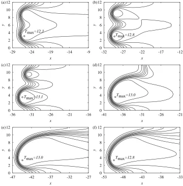
[image:21.612.99.459.86.451.2]x Tmax=12.8 (f)
Figure 7. Temperature profiles (9 equally spaced contours betweenT = 1 and T =Tmax) forW= 12 andλ= 12, at times (a) 9.8, (b) 10.6, (c) 11.4, (d) 12.2,
(e) 13.0, (f) 13.8. The circle marks the point whereT is a maximum in each case.
wavelength.
0 2 4 6 8 10 12
-226 -221 -216 -211 -206
y
x Tmax=12.9 (a)
0 2 4 6 8 10 12
-226 -221 -216 -211 -206
y
x (b)
0 2 4 6 8 10 12
-226 -221 -216 -211 -206
y
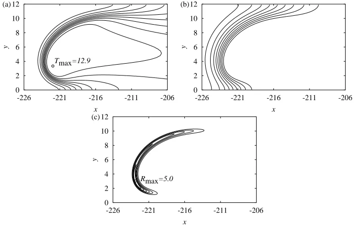
[image:22.612.104.462.86.317.2]x Rmax=5.0 (c)
Figure 8. (a) Temperature (9 equally spaced contours between T = 1 and T = Tmax), (b) fuel fraction (9 equally spaced contours between Y = 0 and
Y = 1) and (c) reaction rate (6 equally spaced contours between R = 0 and R=Rmax) profiles for the nonlinear stationary state whenW = 12 (t= 37.0).
The circles marks the point whereT andRare maximum.
0 3 6 9 12
-1 0 1 2
y
x (a)
0 3 6 9 12
-20 -15 -10 -5 0 5
y
x (b)
Figure 9. Evolution of T = 5 contour for domain width W = 12 and initial perturbation wavelengthλ= 24 at times (a) 1.8, 2.6, 3.4, 4.2 and 5.0 (thex-axis has been stretched by a factor of 7 for clarity) and (b) 5.8, 6.6, 7.4, 8.2, 9.0 and 9.8.
not appear to depend on the initial conditions.
[image:22.612.111.458.391.494.2]0 2 4 6 8 10 12
-26 -21 -16 -11 -6
y
x Tmax=12.4 (a)
0 2 4 6 8 10 12
-30 -25 -20 -15 -10
y
[image:23.612.102.459.88.206.2]x Tmax=12.6 (b)
Figure 10. Temperature profiles (9 equally spaced contours betweenT = 1 and T =Tmax) forW = 12 andλ= 24, at times (a) 11.4 and (b) 12.2.
wavelength corresponding to our λ = 24 ∼ 2λm case, Travnikov et al. (2000) also
found in their Le = 1 calculations that the cell evolved from a half a cell across the domain to a single asymmetric cell. The mechanism in their purely hydrodynamic case appears to be different, in that there is no temperature overshoot, and the new cusp forms in the interior of the domain not at the symmetry line corresponding to the original crest. They found that depending on the thermal expansion this new crest could move towards either the crest or trough of the original symmetric larger cell. Furthermore, the new trough appears much later in the evolution in their case.
Note that for this domain width W = 12 the final cell size agrees with the compatible mode with the largest linear growth rate, in agreement with the results of Kadowaki (1997,1999,2000), Denet and Haldenwang (1995) and Travnikov et al.
(2000), who all used similar sized domains (i.e. W equal to or close toλm). However,
as we shall see below, this agreement with the linear stability predictions in such cases is in general entirely fortuitous and is simply due to the way the solution is restricted by the numerical domain boundaries.
Figure 11 shows the evolution of the flame shape whenW = 18 andλ= 12. As before, each of the initial cells of wavelength 12 split into two smaller cells, breaking the symmetry. In this domain width, the two outer cells created by the splitting grow at the expense of the middle one which disappears, resulting in two cells of wavelength 9. Subsequently the lower of these two cells now grows at the expense of the top one, and hence they merge into a single, asymmetric cell in the domain (figure 11b). Figure 11(c) shows the temperature field in the fully developed cell att= 20.2. In this wider domain, the fold or crack at the top boundary is now markedly deeper, about 30 flame lengths from the position of the crest of the cell. It thus appears that for domain widths of the order ofλmand a choice of symmetry boundary conditions, the
final cell size is determined simply as the largest asymmetric cell which is compatible with the choice ofW, i.e. a single asymmetric cell in the domain.
In order to check this remains true for a still larger domains width, it was necessary to employ lower resolutions. This is because simulations with the highest resolution of 16 points/lf become computationally prohibitive, due not only to the increase
in domain size, but because the flame front becomes increasingly distorted, so that the area over which the finest grid is required becomes larger more rapidly than W
0 3 6 9 12 15 18
-50 -40 -30 -20
y
x (a)
0 3 6 9 12 15 18
-80 -70 -60 -50
y
x (b)
0 3 6 9 12 15 18
-100 -90 -80 -70 -60
y
x Tmax=12.9
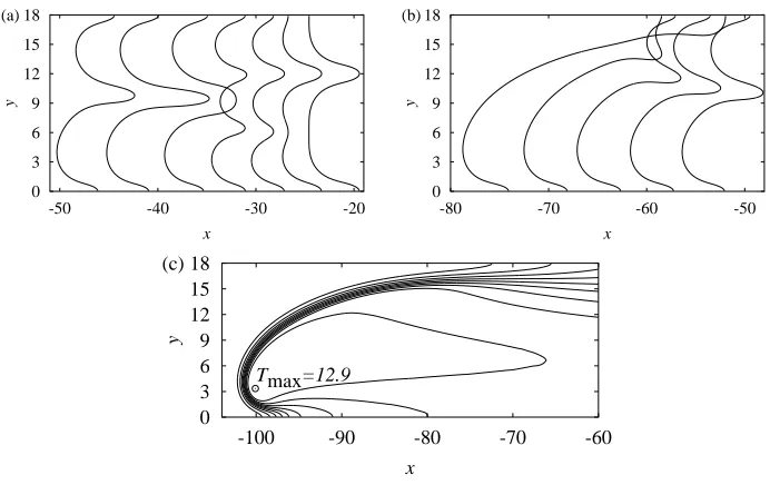
[image:24.612.105.451.86.304.2](c)
Figure 11. Evolution ofT = 5 contour for domain widthW = 18 and initial perturbation wavelength λ= 12 at times (a) 9.0, 9.8, 10.6, 11.4, 12.2, 13.0 and 13.8 and (b) 14.6, 15.4, 16.2, 17.0 and 17.8. (c) Temperature profiles (9 equally spaced contours betweenT = 1 andT =Tmax) forW = 18 andλ= 12, at time
20.2.
0 6 12 18 24
-360 -340 -320 -300 -280
y
[image:24.612.179.384.382.463.2]x Tmax=12.8
Figure 12. Temperature profile (9 equally spaced contours betweenT = 1 and T =Tmax) forW = 24 andλ= 12, at time 43.4. Resolution is 8 points/lf.
domains, we hence used less well resolved calculations with 4 grid refinement levels or 8 point/lf. However, the implicit scheme with 5 refinement levels, but with a
timestep several times that of the explicit scheme, was also used in order to check that the results were not qualitatively different to those of lower spatial resolution explicit scheme results. See§5.1 for spatial and temporal resolution issues.
4.3. Evolution of the outer flow field.
While Kadowaki (1997,1999,2000) concluded that hydrodynamic affects were important for the cellular flame instability, results for the hydrodynamic evolution of the outer flow field were not given. In this section we examine how the nonlinear flame evolution affects this outer flow. One reason it is important to understand the behaviour of the outer flow is because it has ramifications for how the flame will interact with the choice and position of the numerical inflow/outflow boundaries (see
§5.2).
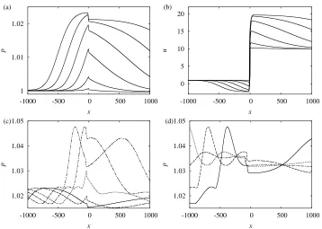
Figure 13(a,b) show the profiles of pressure and component of fluid velocity in thex-direction along the domain centre line (only the region |x|<1000 is shown for clarity)y= 6 for the caseW =λ= 12 (the pressure equilibrates rapidly in the lateral direction, so profiles along other lines of constantyare very similar). The profiles are shown at times during the initial growth stage of the disturbance (cf. figure 4). As the amplitude becomes nonlinear and the flame begins to accelerate, figure 13(a) shows that the pressure levels in the flame also increases. This results in the propagation of pressure (compression) waves fore and aft, away from the flame front into the outer flow field, at the local acoustic speed, i.e. atO(1/Mf) speeds. The resulting pressure
gradients accelerate the fluid, in the negative x-direction ahead of the flame, and in the positivex-direction behind it (figure 13b). Hence the flame sees an evolving fluid speed ahead of it. Note that in this case the fluid velocity just ahead of the flame quickly changes sign: the acceleration of the flame front causes the outer flow field to begin to move away from the initial planar flame position (although of course the nonlinear evolving flame is still moving through the fuel ahead). Figure 13(a) also shows that as the amplitude and flame speed begins to saturate, so does the pressure levels in the flame, and the outer flow field also begins to equilibrate at these levels.
However, figure 13(c) shows that the flame pressure and its affects on the outer flow field begin to evolve again during the splitting process (compare the times shown in figure 13(c) with those in figure 7). As the splitting process begins, the flame speed begins to drop as do the pressures in the flame. It then rapidly re-accelerates as the cell re-merging process begins, and hence the flame pressures also increase once more. Figure 13(c,d) then show that as the flame forms into an single asymmetric cell, there are some rapidly damped oscillations in the flame pressures (and speed) as it relaxes to the final stationary state (note that the pressure profiles in the outer flow ahead and behind the wave provides a history of the prior pressure levels in the flame, since the disturbances propagate away from the flame front at almost constant sound speeds). Figure 2 shows the outer flow fields corresponding the nonlinear stationary state. The important point to note is that the outer flow states ahead and behind the accelerated nonlinear stationary state are quite different from those in the initial planar flame solution.
One would not expect the evolution of the flame to be highly dependent on the choice of initial Mach number, Mf, provided it is small. Indeed, we find this is the
case. However, the evolution of the outer flow field will depend sensitively onMf since
1 1.01 1.02
-1000 -500 0 500 1000
p
x (a)
0 5 10 15 20
-1000 -500 0 500 1000
u
x (b)
1.02 1.03 1.04 1.05
-1000 -500 0 500 1000
p
x (c)
1.02 1.03 1.04 1.05
-1000 -500 0 500 1000
p
[image:26.612.104.462.80.335.2]x (d)
Figure 13.(a) Pressure and (b)x-component of fluid velocity profiles alongy= 6 for W = 12,λ = 12 and timest= 2.6, 3.4, 4.2, 5.0, 5.8 and 6.6. (c) pressure profiles alongy= 6 at times 9.8 (solid line), 10.6 (dashed line), 12.2 (dotted line), 13.0 (dot-dashed line) and 13.8 (double-dot-dashed line). (d) pressure profiles alongy= 6 at times 14.6 (solid line), 16.2 (dashed line), 17.8 (dotted line) and 19.4 (double-dot dashed line).
accelerating flame front). Figure 14, which shows profiles of u along y = 6 for the three different Mach numbers (0.025, 0.005 and 0.001), demonstrates this dependence. As can be seen, asMf increases, the acoustic waves not only take longer to propagate
away from the flame and for the outer flow to equilibrate, but also the amplitude of the disturbances in the outer flow fields become larger (for theMf = 0.025 case the
disturbances actually steepen into very weak shock waves).
Note that from a numerical perspective, for fixedL,Mf also controls the time it
takes for the flame generated flow disturbances to reach the numerical inflow/outflow boundaries and subsequently reflect back to the flame, and hence (together with the truncated domain size) determines the time at which the front becomes in communication with these domain boundaries.
5. Further numerical dependencies.
0 10 20 30
-1000 -500 0 500 1000
u
[image:27.612.196.370.84.209.2]x (d)
Figure 14. Fluid velocity component in thex-direction profiles alongy= 6 when W =λ= 12 forMf = 0.025 (solid line), 0.005 (dashed line), 0.001 (dotted line)
att= 16.2.
results. We then examine the dependence of the solution on the inflow boundary condition and domain length.
5.1. Numerical resolution.
An important question for any numerical simulation is what level of resolution is required to obtain well converged or even qualitatively converged numerical solutions. For flames, the most stringent requirement is to resolve the finest length scale, which is the reaction zone length. As we have seen, the reaction zone in the fully developed nonlinear cells can be much thinner than in the planar wave, so having sufficient resolution to calculate the planar flame problem properly does not mean that this will be sufficient to capture the nonlinear instabilities. Note also that even in the planar flame, the reaction zone length becomes shorter as the Zel’dovich number, β, increases, and rapidly so at large values, thus the resolution requirements will become increasingly stringent for largerβ than used here.
It is worth noting here that Denet & Haldenwang (1995) used a resolution of 4 points/lf in the x-direction (∆x = 0.25 ), Kadowaki (1997) used ∆x=0.2, while
Kadowaki (1999), Travnikov et al. (2002), Kadowaki et al. (2005) and Kadowaki (2000) all used non-uniform grids with the smallest value of ∆x being 0.2, 0.2 and 0.1, respectively.
Figure 15 shows temperature profiles for the caseW =λ= 12, and for resolutions of 4, 8 and 16 points/lf, i.e. ∆x=0.25, 0.125 and 0.0625, respectively, att= 24.2. For
0 2 4 6 8 10 12
-74 -69 -64 -59 -54
y
x Tmax=12.3 (a)
0 2 4 6 8 10 12
-114 -109 -104 -99 -94
y
x Tmax=12.8 (b)
0 2 4 6 8 10 12
-125 -120 -115 -110 -105
y
[image:28.612.102.456.83.330.2]x Tmax=12.9 (c)
Figure 15. Temperature profiles (9 equally spaced contours betweenT = 1 and T =Tmax) forW = 12,λ= 12 at timet= 24.2 and for numerical resolutions of
(a) 4, (b) 8 and (c) 16 points/lf (∆x=0.25, 0.125 and 0.0625, respectively).
flame are not captured properly. One ramification of this is that the acceleration of the outer fluid by the acoustic waves is lessened (see figure 16b). For lower resolution, the flame thus propagates into fuel ahead which is moving more rapidly (in the positive
x-direction), so that the flame speed relative to the initial planar flame is also lower. This is one reason for the large lag in the flame position between figures 15(a) and 15(c). However, note from figure 15 that at the lower resolution, the jump inu1across the flame is underestimate, and hence so is the flame speed with respect to the rest frame of the upstream fluid.
However, figures 15 and 16 also show that the solution is rapidly converging as the resolution increases. The results for 8 and 16 points/lf are in good agreement,
indicating that our solution with 16 points/lf is well converged. For such narrow
domains (similar to those used in previous simulations), it thus appears that very little resolution is required to obtain the qualitatively correct evolution and final state.
However, in for larger domain widths, sufficient resolution is more crucial for obtaining the qualitatively correct solution. Figure 17 shows the temperature profiles for W = 18 and λ = 12 at t = 20.2 and for resolutions of 8 and 4 points/lf (4
and 3 grid refinement levels, respectively). The 8 point/l1/2 case is still in good agreement with the higher resolution solution, compare figure 17(a) with 11(c) when 5 refinement levels were used, but note again the lag in the flame position, the slight underestimate of the maximum temperature and the smaller depth of the fold at the upper boundary for 8 as compared to 16 points/lf cases. However, now the lowest
1.02 1.03 1.04
-1000 -500 0 500 1000
p
x (a)
0 10 20 30
-1000 -500 0 500 1000
u
[image:29.612.106.460.85.214.2]x (b)
Figure 16. (a) Pressure and (b)x-direction component of fluid velocity profiles alongy= 6 forW = 12,λ= 12 and timet= 24.2 and for numerical resolutions of 4 (solid lines), 8 (dashed lines) and 16 (dotted lines) points/lf.
0 3 6 9 12 15 18
-90 -80 -70 -60
y
x Tmax=12.8 (a)
0 3 6 9 12 15 18
-65 -55 -45 -35 -30
y
x Tmax
=13.0 (b)
Figure 17. Temperature profiles (9 equally spaced contours betweenT = 1 and T =Tmax) forW= 18 andλ= 12 at timet= 20.2 and for numerical resolutions
of (a) 8 and (b) 4 points/lf
at time t = 20.2. We have ran this low resolution case for very long times and the flame never approaches a stationary state. Instead the flame front continually cycles through irregular cell splitting and re-merging events. It thus appears in wide enough domains, a single large cell cannot be sustained at low resolutions, presumably because the reaction zone lengths in this single cell solution are not being resolved. This non-stationary cyclic behaviour of cell splittings and mergings is also seen in the results of the very wide domain simulations of Kadowakiet al. (2005) whenLe= 0.5. Note that Kadowakiet al. (2005) used a similar resolution to our low resolution case in the
x-direction, but also used a larger Zel’dovich number than that employed here. This suggests that their time-dependent results may thus also be due to under-resolution, and hence one should be cautious in interpreting their physical relevance.
In order to examine the role of temporal accuracy in the numerical solution (as well as to provide cross-validation of the results with the explicit solver), cases were examined using the implicit timestep solver with increasing timesteps, but the resolution fixed at 16 points/lf. Figure 18 shows the cellular flame at t = 24.2 for
[image:29.612.105.451.271.356.2]