Multiscale modelling tool : mathematical modelling of collective behaviour without the maths

White Rose Research Online URL for this paper:

http://eprints.whiterose.ac.uk/153014/

Version: Published Version

Article:

Marshall, J.A.R. orcid.org/0000-0002-1506-167X, Reina, A. and Bose, T. (2019) Multiscale

modelling tool : mathematical modelling of collective behaviour without the maths. PLOS

ONE, 14 (9). 0222906.

https://doi.org/10.1371/journal.pone.0222906

[email protected] https://eprints.whiterose.ac.uk/

Reuse

This article is distributed under the terms of the Creative Commons Attribution (CC BY) licence. This licence allows you to distribute, remix, tweak, and build upon the work, even commercially, as long as you credit the authors for the original work. More information and the full terms of the licence here:

https://creativecommons.org/licenses/

Takedown

If you consider content in White Rose Research Online to be in breach of UK law, please notify us by

Multiscale Modelling Tool: Mathematical

modelling of collective behaviour without the

maths

James A. R. MarshallID*, Andreagiovanni ReinaID, Thomas Bose

Department of Computer Science, University of Sheffield, Sheffield, United Kingdom

*[email protected]

Abstract

Collective behaviour is of fundamental importance in the life sciences, where it appears at levels of biological complexity from single cells to superorganisms, in demography and the social sciences, where it describes the behaviour of populations, and in the physical and engineering sciences, where it describes physical phenomena and can be used to design distributed systems. Reasoning about collective behaviour is inherently difficult, as the non-linear interactions between individuals give rise to complex emergent dynamics. Mathemati-cal techniques have been developed to analyse systematiMathemati-cally collective behaviour in such systems, yet these frequently require extensive formal training and technical ability to apply. Even for those with the requisite training and ability, analysis using these techniques can be laborious, time-consuming and error-prone. Together these difficulties raise a barrier-to-entry for practitioners wishing to analyse models of collective behaviour. However, rigorous modelling of collective behaviour is required to make progress in understanding and apply-ing it. Here we present an accessible tool which aims to automate the process of modellapply-ing and analysing collective behaviour, as far as possible. We focus our attention on the general class of systems described by reaction kinetics, involving interactions between components that change state as a result, as these are easily understood and extracted from data by nat-ural, physical and social scientists, and correspond to algorithms for component-level con-trollers in engineering applications. By providing simple automated access to advanced mathematical techniques from statistical physics, nonlinear dynamical systems analysis, and computational simulation, we hope to advance standards in modelling collective behav-iour. At the same time, by providing expert users with access to the results of automated analyses, sophisticated investigations that could take significant effort are substantially facil-itated. Our tool can be accessed online without installing software, uses a simple program-matic interface, and provides interactive graphical plots for users to develop understanding of their models.

a1111111111 a1111111111 a1111111111 a1111111111 a1111111111

OPEN ACCESS

Citation:Marshall JAR, Reina A, Bose T (2019) Multiscale Modelling Tool: Mathematical modelling of collective behaviour without the maths. PLoS ONE 14(9): e0222906.https://doi.org/10.1371/ journal.pone.0222906

Editor:Jonathan David Touboul, Brandeis University, UNITED STATES

Received:July 1, 2019

Accepted:September 10, 2019

Published:September 30, 2019

Peer Review History:PLOS recognizes the benefits of transparency in the peer review process; therefore, we enable the publication of all of the content of peer review and author responses alongside final, published articles. The editorial history of this article is available here:

https://doi.org/10.1371/journal.pone.0222906

Copyright:©2019 Marshall et al. This is an open access article distributed under the terms of the

Creative Commons Attribution License, which permits unrestricted use, distribution, and reproduction in any medium, provided the original author and source are credited.

Data Availability Statement:All software is available from GitHub (https://github.com/ DiODeProject/MuMoT).

Introduction

Collective behaviour models, in which individuals interact and in doing so change state, describe a large variety of physical, biological, and social phenomena. One particularly general formulation is that ofreaction kinetics, developed to describe the time evolution of chemical reactions, but also able to describe networks in molecular biology (e.g. [1]), collective beha-vioural phenomena such as decision-making in animal groups (e.g. [2]), demographic and eco-logical models such as predator-prey dynamics (e.g. [3]), epidemiological models (e.g. [3]), and social behaviour in human groups, such as opinion dynamics and economics (e.g. [4]). The generality of the reaction kinetics formalism is demonstrated by the fact that many of the afore-mentioned processes, although apparently quite different, are in fact described by the same dynamical equations; for example, the famous Lotka-Volterra equations were simultaneously developed in the description of a chemical reaction, and predator-prey dynamics [5,6].

Modelling collective behaviour is essential to develop understanding, yet mathematical and computational modelling are skills than can be found in some disciplines much more than others. To understand commonalities and analogies across disciplines it would be beneficial to ensure a consistent standard of modelling is reached across all. However, it is unreasonable to expect all disciplines to ensure the same standard of mathematical training in their practition-ers. Reaction kinetics have the advantage that they describe observations of a system in a very natural way, indeed the very way that experimental scientists tend to record those interactions. Reaction kinetics can also be transformed into mathematical equations according to a variety of procedures. The level of description attainable may vary, however. In their simplest form, mathematical models as Ordinary Differential Equations will assume infinitely large, well-mixed populations; thismean-fieldapproach ignores fluctuations in subpopulation sizes due to the stochastic effects that small populations entail, and also ignores spatial heterogeneity and attendant sources of noise. Yet ODEs are analytically most tractable, and so enable general insights to be developed into the behaviour of an idealised version of the system of interest. By introducing finite population effects, noisy fluctuations around the mean-field solution can be studied; these can be approximated analytically, through the application of techniques from statistical mechanics, or numerically through efficient and probabilistically correct simulation of the Master Equation, which gives the continuous-time change in the probability density over the possible states of the system. These approaches are still idealisations, in that they ignore noise due to spatial effects, but they retain some tractability. Finally, one may analyse spatial sources of noise, by embedding a finite population in a spatial environment, such as a network, or a 2-dimensional plane or 3-dimensional volume. While in some cases analytic results may be possible, particularly in the case of networks, in general numerical simulation is required, sometimes referred to as Individual-Based Simulation or Agent-Based Simulation. This approach is therefore the most realistic, while also the least analytically tractable. In understanding the collective behaviour of some real-world system, therefore, the approach is generally to understand the simplest model of the system, then progressively introduce more realistic sources of noise in order to see if that behaviour is changed in important ways.

Taking all of the above points into consideration, we here present a Multiscale Modelling Tool, intended to simplify as much as possible the application of analytic and numerical tech-niques to descriptions of simple collective behaviour systems. The tool has the following objec-tives, and in the remainder of the paper we describe how these are achieved:

1. enable non-modellers to describe collective behaviour systems intuitively

2. enable a variety of analyses to be applied easily to such systems, accounting for increasingly realistic sources of noise

europa.eu) under the European Union’s Horizon 2020 research and innovation programme (grant agreement number 647704). The funders had no role in study design, data collection and analysis, decision to publish, or preparation of the manuscript.

a. infinite-population non-spatial noise-free dynamics

b. non-spatial finite-population noisy dynamics

c. spatial finite-population noisy dynamics

3. enable interactive exploration of analysis results

4. enable expert-level access to analysis results

5. minimise overheads for installation and use of the software

Design and implementation

MuMoT (Multiscale Modelling Tool) is written in Python 3 [7] and designed to be run within Jupyter notebooks [8]. This enables MuMoT to be used in interactive notebook sessions using widgets, with explanations written in Markdown and LATEX to develop interactive computa-tional documents, particularly suited to communication of results and concepts in research or teaching environments. A Jupyter notebook server can be deployed with a MuMoT installa-tion to allow users to work through a standard web browser, without the need to install client-side software, facilitating access and uptake; at the time of writing, the interactive MuMoT user manual can be executed in this mode via Binder [9] (see [10]). Despite being primarily designed for interactive use, MuMoT uses a variant of the Model, View, Controller design pat-tern [11] enabling a separation between model descriptions, analytic tools applied to models, and interactive widgets for manipulation of analyses; this enables MuMoT to be used non-interactively, for example with routines called directly from user code.

As MuMoT runs in Jupyter notebooks the user enters simple commands in notebook cells. Models are generated from intuitive textual descriptions, or from mathematical manipulation of previously-defined models, and most commands applicable to models result in interactive graphical output. To enable users to concentrate on presenting the key relevant concepts, users can partially or totally fix parameters in the resulting controllers, and have single controllers connected to multiple model views, with nesting of views if desired [10].

MuMoT’s implementation, testing, and documentation seeks to adhere to the best stan-dards for scientific software deployment [12,13].

Specifying collective behaviour models

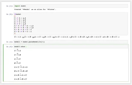
Users describe models as simple textual rules, standard in the description of reaction kinetics. We refer to individuals asreactantswhich can be, for example, different classes of individuals as in the case of chemical molecules or members of different biological species, or individuals having different changeable states as in the case of voter models, or robot swarms. Rules describe which reactants interact with each other, the resulting reactants, and the rate at which such reactions occur. For example,Fig 1shows the description of a model of collective deci-sion-making in honeybee swarms [2,14] within MuMoT, and how this is parsed into a mathe-matical object.

Models can also be created from the mathematical manipulation of other models; for exam-ple, it can be convenient to note that the frequency of one of the reactants can be determined from the frequencies of the remaining reactants, and the total system size, in any closed system where no reactant can be created or destroyed:

model2 = model1.substitute(’U = N - A - B’)

model3 = model2.substitute(’a_A = 1/v_A, a_B = 1/v_B, g_A = v_A, g_B = v_B, r_A = v_A, r_B = v_B’)

or even in terms of the mean and difference between those qualities [2,14]:

model4 = model3.substitute(’v_A = \mu + \Delta/2, v_B = \mu -\Delta/2’)

Once parsed, a model exists as a mathematical object ready for analysis, as can be seen by asking to see the Ordinary Differential Equations (ODEs) that describe its time evolution:

model4.showODEs()

which results in the following system of equations:

dA

dt ABsþA D

2þm

� �

A B_þN

ð Þ DA

2þm

þ D₂þm

� �

A B_þN

ð Þ;

dB

dt ABsþB D

2þm

� �

A B_þN

ð Þ DB

2þm

þ D₂þm

� �

A B_þN

ð Þ:

ð1Þ

Eq 1have been automatically derived from the rule-based description of the model we pro-vided. Two techniques can be used to derive these ODEs, either amass actionheuristic similar to the one a mathematician would use to derive the ODEs, or a more involved statistical phys-ics approach described in section ‘Analysing noisy behaviour’ (e.g. [15]). Both, however, have the same result.

Fig 1. Specification of a collective behaviour model.A model is described using simple textual rules denoting interactions between reactants in the system, and rates and which they are transformed into new combinations. Parsing this model description automatically results in a mathematical model object ready for analysis.

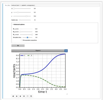
Once a model has been parsed, a variety of analytic and numerical techniques can be applied to it. Many of these result in interactive graphical displays of the analysis, which users can manipulate to explore their model. For example,Fig 2shows the result of performing a numerical integration on the model ofEq 1within the notebook environment, using the

integrate()command. Although not described in this paper, parameters can be fixed as

desired to focus on a particular set of free parameters (partial controllers), and multiple views on the same model can be manipulated via a single controller (multicontroller). Users can also bookmarkinteresting parameter combinations to reproduce subsequently, and save the results from some views for analysis in external software packages. Such devices allow researchers and teachers to focus exploration and exposition of important concepts. Full details are given in the online user manual [10].

Analysing noise-free infinite population behaviour

The most analytically tractable means of analysing collective behaviour are typically those that assume infinite populations; in this mean-field approach sources of intrinsic noise due to finite population effects are neglected, and space is also ignored. Thus understanding the noise-free

Fig 2. Interactive manipulation of a model view via a controller.Most model analysis commands result in an interactive graphical display of that analysis on the model. Users can explore and visualise the effects of changing free model parameters, and other analysis-specific parameters, through manipulating interactive controls.

dynamics of a collective behaviour system is normally the most fruitful starting point in deal-ing with any new system.

Numerical integration of ODEs and phase portraits. The simplest way to approach the

noise-free dynamics of a system is often to integrate the ODEs that describe it. To achieve this MuMoT provides theintegrate()method, which makes use of theodeintinterface to numerical integrators implemented in Python’s SciPy packagescipy.integrate[16]. Solutions are displayed as interactive graphical output (see for exampleFig 2). Plots can be pre-sented either in terms of absolute numbers, or of population proportions (i.e. the number of ‘particles’ for eachreactantdivided by the system size att= 0).

The dynamics of a MuMoT model can also be studied by means of aphase plane analysis. To visualise the model’s trajectories in aphase portraitthe methodsstream()

andvector()can be applied. Both methods depict phase planes representing the time

evolution of the system as a function of its state; in a vector plot arrows give the direction in which the system will move, and their lengths show how fast, whereas in a stream plot lines show the average change of the system over time in finer resolution, and their shading repre-sents the speed of change. It is also possible to calculate and display fixed points and noise around these; the corresponding theory and computations are introduced below. Stream plot examples are shown inFig 4. More detailed explanations can be found in the online user manual [10].

Bifurcations. Nonlinear dynamical systems may change behaviour qualitatively if model

parameters are varied. To detect such transitions between different dynamic regimes MuMoT implements basicbifurcation analysisfunctionality by integrating with PyDSTool [17]. MuMoT’s method enabling bifurcation analysis is calledbifurcation(). Currently avail-able is the detection ofbranch points(BPs) andlimit points(LPs) of one-dimensional and dimensional systems; remember that a three-dimensional system may be reduced to a two-dimensional one using MuMoT’ssubstitute()method. Detectable bifurcation points in MuMoT belong to the class of local codimension-one bifurcations. For example, BPs are observed forpitchforkbifurcations such as the one shown inFig 5(left panel).Saddle-node bifur-cations are typical LPs (Fig 5(middle and right panels)). For two-dimensional systems it may be desirable to directly compare the behaviour of both dynamical variables (orstate variablesas we call them within MuMoT) depending on a critical parameter in the same two-dimensional plot, where the bifurcation parameter is plotted on the horizontal axis. MuMoT allows users to plot single reactants as response variables, but also sums or differences of reactants, as illustrated in Fig 5(left panel). For more information on the usage ofbifurcation()we refer the reader to the online user manual [10].

Analysing noisy behaviour

Any real-world system is subject to noise, hence the next step in analysing a collective behav-iour system is to examine deviations from the mean-field solutions of the model under such noise. There are two primary sources of noise, that due to finite population size, and that due to spatial distribution of the population; MuMoT enables analysis of both.

Finite-population noise. We start with intrinsic noise, due to finite population size. In

any finite system the number of interactions fluctuates around an average value and hence so do the numbers of agents in the states available. The following derivation is based on the classi-cal textbook by van Kampen [18]. In analogy to a typiclassi-cal chemiclassi-cal reaction let us consider a system of interacting agentsXkwithk= 1, 2. . .,Kbeing the different states agents might be in.

HereXdenotes the type of agent and the state represented by indexkmay be the commitment state. For example this could be a honeybee advertising a potential new nest site. The number of agents in statekis denotednk; when agents interact the numbers in any statekmay change.

Using integer stoichiometric coefficients denoted kand kthe change of the system’s state

fol-lowing interactions may be described by

a1X1þa2X2þ � � � !b1X1þb2X2þ � � � ; ð2Þ

where the left-hand side characterises the state before the interaction (reaction) and the right-hand side the state after the interaction (reaction). All interaction processes are affected by the total number of agents. To account for this, we introduce the system sizeV as a formal (auxil-iary) parameter that is necessary for the following derivation.

The Master equation. In order to sufficiently describe our system of interest, we need to

compute the averaged macroscopic numbers and we also need to quantify the fluctuations around these averaged quantities. This may be achieved by means of the chemical Master equation, which can be written as follows [18]:

@P_ðfn_kg;t_Þ

@t ¼

X

i

rðiÞ þV

Y

k

EaðkiÞ b

ðiÞ

k

k 1

! Y

j

ððnjÞÞ

aðiÞ j

VaðjiÞ

0

@

1

APðfn_kg;tÞ 0

@

þrðiÞ_V Y

k

EbðiÞ k að

iÞ k k 1 ! Y j

ððnjÞÞ

bðiÞ j

VbðjiÞ

0

@

1

APðfn_kg;tÞ 1

A;

ð3Þ

whereEis the step operator ([18], chapter VI, Eq 3.1),∑irepresents the sum over all reactions

i, and rate superscripts (i) denote the rates for reactioni. The first term in the sum on the right-hand side represents reactions as inEq (2)(proportional to a constant interaction rate r_þðiÞ) and the second term their inverse reactions (proportional to constant interaction raterðiÞ_). Note that the inverse reaction does not always exist. If it exists, in a MuMoT model definition this would simply be written as an expression like the one inEq (2),i.e. the convention used in MuMoT strictly followsEq (2). For example, see input cellIn[2]inFig 1; there are also several examples in the online user manual to show how this works [10]. The expression

ððnjÞÞ

a_j

¼nj!=ðnj ajÞ!is introduced as an abbreviation.Eq (3)describes the temporal

evolu-tion of the joint probability distribuevolu-tion that the system under study is in state {nk} at timet.

Here, {nk} summarises all agents’ individual states as a set. To express changes following

inter-actions we make use of step operatorsEkwhich increase or decrease the number of agents

van Kampen expansion of the Master equation. In general, there are only very few examples for whichEq (3)can be solved exactly. In what follows we describe an approximation method known assystem size expansionorvan Kampen expansionthat yields analytical expres-sions to approximate the solution of a Master equation. However, here we only introduce the main idea of the expansion method and refer to van Kampen’s textbook [18] for further details. LetFXk¼Xk=Vdenote the proportion of the populationXkgiven the system sizeV.

Note thatFis a reserved symbol in MuMoT used to express population proportions—the ana-logue to concentrations of reactants in a chemical reaction. The probability to observe the sys-tem in statenkhas a maximum around the macroscopic variableFXkwith a deviation around

that maximum of order iiiii_n

k

p _� iiii

V

p

[18]. We may now replace the numbernkby a new

ran-dom variable, sayZ_X

k, according to [18]

nk¼VFX_kþ

iiii V

p

ZX_k: ð4Þ

This also means that the probability distributionPneeds to be rewritten in the new variables, i.e.Pðfnkg;tÞ !PðfZXkg;tÞ. Accordingly, the step operatorsEinEq (3)are expanded to

yield [18]

E¼1_þ 1iiii V

p _@Z@

Xk

þ 1

2V

@2 @Z2

X_k

þ � � �: _ð5Þ

Calculating the time derivative ofP_ðfZ_X

kg;tÞby applying Eqs (4) and (5) toEq (3)it is possible

to get the equation forPðfZ_X

kg;tÞexpressed in terms of different orders of the systems size V(note that theZX_kare time-dependent viaFX_kinEq(4)). As a result, there are large terms

/piiiiVwhich should cancel, yielding the macroscopic equation of motion forFXk. This

corre-sponds to directly deriving the macroscopic ODE forFXkfrom the underlying reaction by

applying thelaw of mass action. The next highest order in this expansion is_/V0_{. Collecting}

all terms_/V0_{and neglecting all other terms (}

�O_ðV 1=2

Þ) yields a Fokker-Planck equation with terms linear inZ_X

k(linear noise approximation). Although we do not attempt to solve

Master equations or their approximations in the form of linear Fokker-Planck equations in MuMoT, we utilise the linear Fokker-Planck equation to compute analytical expressions that represent fluctuations and noise correlations, by deriving equations of motion for first and sec-ond order moments ofPðfZ_X

kg;tÞaccording to @

@thZXiiðtÞ ¼

Z d Z_X

i @

@tPðfZXkg;tÞ;

@

@thZXiZXjiðtÞ ¼

Z d Z_X

iZXj @

@tPðfZXkg;tÞ;

ð6Þ

whered _¼dZX1� � �dZXK, and@P/@trepresents the linear Fokker-Planck equation. Both van

Kampen expansion and derivation of the linear Fokker-Planck equation can be readily per-formed in MuMoT. In addition, in MuMoT explicit expressions for first and second order moments following fromEq (6)may be derived. Furthermore, MuMoT can attempt to obtain analytical solutions for these equations in the stationary state.

All mathematical procedures concerning the Master equation and Fokker-Planck equation make extensive use of Python’s SymPy package [19].

Other methods to study noise in MuMoT. Making use of MuMoT’s functionality

evolution of correlation functionshZ_X

kðtÞZXjð0Þi; examples of how to do this are given in the

online user manual [10]. Noise can also be displayed in stream and vector plots; if requested then MuMoT tries to obtain the stationary solutions of the diagonal elements of the second order moments and then project these onto the direction of the eigenvectors of available stable fixed points of the macroscopic ODEs. If the system is too complicated and MuMoT cannot find an analytical solution, noise may be calculated by principled numerical simulation, as described below.

Stochastic simulation. The Master equation ofEq (3)can be very difficult to solve for

even very simple systems, therefore most studies resort to the complementary approach of numerical simulations [20]. Gillespie proposed a probabilistically exact algorithm for simulat-ing chemical reactions called thestochastic simulation algorithm(SSA) [21]. Each simulation computes a stochastic temporal trajectory of the state variables from a given user-defined ini-tial condition@P({nk}; 0) for a user-defined maximum timeT. Averaging various trajectories

gives an approximation of the solution ofEq (3)(for a given@P({nk}; 0)) that increases in

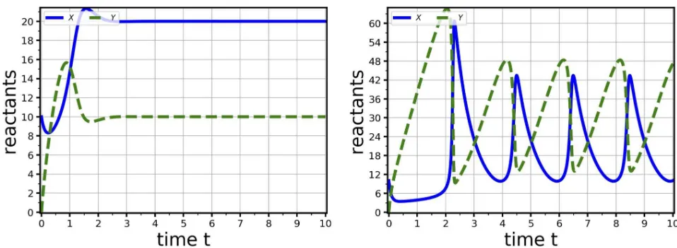
accu-racy with the number of simulations. MuMoT implements the SSA via the commandSSA(). The user can run a single simulation to generate a single temporal trajectory, or otherwise run several simulations and aggregate the data in a single plot. The user can visualise the entire temporal trajectory (in a plot similar toFig 3), or the final population distribution@P({nk};T)

in the form of either a barplot or as points in a 2-dimensional space plane (in which the two axes are state variables). Multiple trajectories can be aggregated in standardised ways of dis-playing probability distributions,e.g., in the 2-dimensional space plane, simulation aggregates are visualised as ellipses centred on the distribution mean and with 1-σcovariance sizes (e.g. see the green ellipse inFig 4(bottom panels)). This aggregate visualisation can be superim-posed on to stream and vector field plots when requested, and ifEq (3)cannot be analytically solved by MuMoT, as discussed above.

Spatial noise. MuMoT also enables the study of the effects of spatial noise on a model.

Including spatial noise relaxes the sometimes simplistic assumption of a well-mixed system in which interactions between any group of reactants can always happen, at rates proportional to the product of their relative frequencies in the population. Instead, each reactant has a set of availablereactants with which it can interact at each timestep. The set of possible interactions

Fig 3. Numerical integration of the Brusselator equations.The Brusselator equations ([3], p.253) exhibit either stable (left) or oscillatory (right) dynamics according to the parameter values selected. Parameter sets:F =F = = = =ξ= 2.0,FXt(0)= 1.0, system size = 10 (left),F = = = =ξ = 2.0,F = 5.5,FXt(0)= 1.0, system size = 10 (right).

corresponds to the system’s interaction topology, which the user can select among a set of stan-dard graph structures. Graphs are handled by MuMoT through the functionalities offered by the NetworkX library [22] which allows advanced users to easily add new topologies. In the first MuMoT release, the available topologies are the complete graph, the Erdo¨s–Re´nyi random graph [23], the Baraba´si–Albert scale-free network [24], and the random geometric graph [25]. The latter is constructed by locating at random uniform locations the reactants in a square environment with edge length 1, and allowing interaction between two reactants when their Euclidean distance is less than or equal to a user-defined distance. The topology of the random geometric graphs can be static or time-varying. The latter is implemented by letting each reac-tant perform a correlated random walk in the 2-dimensional environment and recomputing the topology each time based on the new distances between reactants.

Spatial noise is difficult to compute analytically in an automatised way, therefore MuMoT computes it numerically via individual-based simulations. Each reactant is simulated as an agent which probabilistically interacts at synchronous discrete timesteps with the available

Fig 4. Phase portraits with computed fixed points and noise.Upper-left: oscillatory dynamics in the Lotka-Volterra equations ([3], p.79) (parametersFA= = = = 2.0). Upper-right: limit cycle in the Brusellator ([3], p.253) (parametersF = = = =ξ= 2.0,F = 5.5). Lower-left: global attractor with isotropic noise in the Brusellator ([3], p.253) (parametersF =F = = = =ξ= 2.0, system size = 10). Lower-right: co-existence of two stable attractors in the honeybee swarming model [2], with anisotropic non-axis-parallel noise (parametersΔ= 0.0,μ= 3.0,s= 10.0, system size = 20, runs = 100). Line shading indicates speed of flow, with darker representing faster. Fixed points are denoted as stable (dark solid green circle), saddle (hollow blue circle), or unstable (hollow red circle). Light green ellipses represent 1-σnoise around stable fixed points.

reactants. The agent’s behaviour is automatically implemented from the model’s reaction kinetics as a probabilistic finite state machine following the technique proposed in [26]. Along with the agents’ behaviour, MuMoT automatically sizes the timestep length to match the time-scale with the population-level descriptions (e.g. ODEs and Master equation). This feature can be particularly convenient if the user aims at a quantitative comparison between model description levels. Similarly to SSA simulations, the user can select to run individual simula-tions or to aggregate results from multiple independent simulasimula-tions to compute statistical distributions.

Results

All results can be reproduced using theMuMoTpaperResults.ipynbJupyter notebook [10].

Numerical integration

To illustrate the numerical integration functionality of MuMoT we repeat analyses of the Brus-selator equations ([3], p.253) inFig 3. The equations have two dynamical regimes, one with a single globally stable attractor whenFb�F

2

a(Fig 3(left)), and one in which a stable limit

cycle exists whenFb>F

2

a(Fig 3(right)).

Phase portraits with fixed point and noise calculations

We illustrate the phase portrait functionality of MuMoT inFig 4by repeating analyses of a variety of equation systems: the classical Lotka-Volterra equations ([3], p.79), the Brusellator equations ([3], p.253), and a model of collective decision-making by swarming honeybees [2, 14]. These systems can exhibit a variety of dynamics including: oscillations (Fig 4(upper-left)), unstable fixed points with limit cycles (Fig 4(upper-right)), globally stable attractors (Fig 4 (bottom-left)), and stable attractors co-existing with saddle points (Fig 4(bottom-right)). When stable fixed points are present MuMoT can calculate or compute the equilibrium noise around them, dependent on system size (Fig 4(bottom)); this can be either isotropic (Fig 4 (bottom-left)), or anisoptropic and/or non-axis-parallel (Fig 4(bottom-right)). This latter case is particularly interesting because the correct noise around the fixed point may differ substan-tially from simply adding Gaussian noise to the dynamical equations.

Bifurcation analysis

MuMoT’s bifurcation analysis functionality is illustrated through reproducing a number of bifurcation analyses [14] of the honeybee model presented above [2] (Fig 5). These reveal con-ditions under which the dynamics exhibit: (i) a pitchfork bifurcation (Fig 5(left)), a sample post-bifurcation phase portrait for which is presented inFig 4, (ii) an unfolding of the pitch-fork bifurcation (i.e. saddle-node bifurcation) (Fig 5(centre)), and (iii) a hysteresis loop (Fig 5 (right)). These can be compared to figures 5(i)-(iii) of [14].

Finite population and spatial numerical simulation

Derivation of the Master equation and expansion to derive the

Fokker-Planck equation

Here we reproduce the analysis presented in [18] (pp. 244-246) to derive the Master Equation and Fokker-Planck equation for the following toy model:

ðA_{Þ !}k X

X_þX_!h _{; þ ; ð}7Þ

The automated analysis results in

@ @tP Xð ;tÞ

Ak

V ðEopðX; 1Þ 1ÞV P Xð ;tÞ þhðEopðX;2Þ 1Þ X

VðX 1ÞP Xð ;tÞ ð8Þ

Fig 6. Numerical simulations of a nonlinear decision-making model.Numerical simulations of the honeybee swarming model [2,14] given various sources of noise. Left: finite-population noise effects during symmetry-breaking in a well-mixed model (cf. [14] Movie S1) (parametersΔ= 0,μ= 3.0,

s= 3.0,FUt(0)= 1.0, system size = 50, time = 10, runs = 10). Centre: finite-population and spatial noise effects due to embedding the model in a random graph. Right: finite-population and spatial noise effects due to embedding the model in a plane, with agents performing correlated random walks; traces indicate recent agent paths, links indicate current interaction events.

https://doi.org/10.1371/journal.pone.0222906.g006

Fig 5. Bifurcation analysis of a nonlinear decision-making model.Bifurcations of the honeybee swarming model [2,14]. Left: symmetry breaking in the two decision populations through a pitchfork bifurcation, with strength of cross-inhibitory stop-signallingsas the bifurcation parameter (cf. [14] Fig 5i) (parametersΔ= 0.0,μ= 4.0). Centre: unfolding of the pitchfork bifurcation into a saddle-node bifurcation (cf. [14] Fig 5ii) (parametersΔ= 0.1,μ

= 4.0). Right: hysteresis loop with option quality differenceΔas the bifurcation parameter (cf. [14] Fig 5iii) (parametersμ=s= 4.0). Solid black lines denote stable branches, dashed blue lines denote unstable branches.

and

@

@tPðZX;tÞ

FAk

2 @2 @Z2

X

PðZ_X;tÞ þ2F2

Xh

@2 @Z2

X

PðZ_X;tÞ þ4FXZXh

@ @ZX

PðZ_X;tÞ þ4FXhPðZX;tÞ ð9Þ

as expected.

A substantially more complicated example derivation, for the honeybee swarming model of Eq 1[2,14], is presented inS1 Text. This derivation is equivalent to that performed in [2] and results in the same dynamical equations.

Availability and future directions

MuMoT is available as source code, as a package for Python 3 [27] via PyPI (pypi.python.

org), and as a server-based installation currently exemplified by free-to-use access to the interactive user manual and other notebooks using the Binder service [9], which requires only a web browser to use. MuMoT is written in Python 3 and integrates with Jupyter Notebooks [8] and as such is platform-independent. Non-interactive aspects of MuMoT’s functionality can also be accessed through using it as a standalone Python package, enabling its modelling and analysis functionality to be used from within third-party code projects. MuMoT is avail-able under the GPL licence version 3.0, and makes use of other software availavail-able under the MIT licence. For further details including links to usage information are available at

github.com/DiODeProject/MuMoT/.

Numerous software products have been proposed to perform subsets of the analyses offered by MuMoT. For instance, several tools offer the possibility to run the SSA and efficiently ana-lyse reaction kinetics models [28–36]. Similarly, software to anaana-lyse mean-field dynamical sys-tems and perform bifurcation analysis is widely available,e.g. MATCONT for Matlab [37], or the Dynamica package for Wolfram Mathematica [38]. Linear noise approximations have pre-viously been implemented as well [32]. Several tools offers software to simulate complex sys-tems, dynamical networks, and agent-based models [39–41], some of which run as Jupyter notebooks as MuMoT does [42,43].

In contrast to the previous solutions, MuMoT combines ease-of-use with a multi-level anal-ysis that spans from ODEs analanal-ysis, to statistical physics approximations, bifurcation analanal-ysis, and SSA and multiagent simulations, integrated within a simple interactive notebook docu-ment interface. This makes MuMoT particularly appropriate for non-experts to learn to build models and apply complex mathematical and computational techniques to them, to communi-cate research results, and to enable students to interactively explore models, and modelling and analysis techniques.

Supporting information

S1 Text. Sample model analyses.van Kampen expansion and other analyses of the stop-signal

model (Eq 1). (PDF)

Acknowledgments

We thank Will Furnass with assistance in deployment, documentation, and continuous inte-gration. We thank Renato Pagliara for assistance in testing on the Windows platform.

Author Contributions

Conceptualization:James A. R. Marshall.

Formal analysis:Thomas Bose.

Funding acquisition:James A. R. Marshall.

Methodology:James A. R. Marshall, Andreagiovanni Reina, Thomas Bose.

Project administration:James A. R. Marshall.

Software:James A. R. Marshall, Andreagiovanni Reina, Thomas Bose.

Validation:James A. R. Marshall, Andreagiovanni Reina, Thomas Bose.

Writing – original draft:James A. R. Marshall, Andreagiovanni Reina, Thomas Bose.

Writing – review & editing:James A. R. Marshall, Andreagiovanni Reina, Thomas Bose.

References

1. Tyson JJ, Chen KC, Novak B. Sniffers, buzzers, toggles and blinkers: dynamics of regulatory and sig-naling pathways in the cell. Current Opinion in Cell Biology. 2003; 15(2):221–231.https://doi.org/10. 1016/s0955-0674(03)00017-6PMID:12648679

2. Seeley TD, Visscher PK, Schlegel T, Hogan PM, Franks NR, Marshall JAR. Stop signals provide cross inhibition in collective decision-making by honeybee swarms. Science. 2012; 335(6064):108–111.

https://doi.org/10.1126/science.1210361PMID:22157081

3. Murray JD. Mathematical Biology I: An Introduction. 3rd ed. Springer-Verlag; 2002.

4. Yildiz E, Ozdaglar A, Acemoglu D, Saberi A, Scaglione A. Binary opinion dynamics with stubborn agents. ACM Transactions on Economics and Computation (TEAC). 2013; 1(4):19.

5. Israel G. La Mathe´matisation du Re´el. Seuil; 1996.

6. Marshall JAR, Franks NR. Computer modeling in behavioral and evolutionary ecology: whys and wherefores. In: Modeling Biology: Structures, Behavior, Evolution. The Vienna Series in Theoretical Biology. MIT Press; 2007. p. 335–353.

7. van Rossum G, et al. Python 3; 2008. Available from:https://www.python.org/3/reference/; accessed on 2019-06-12 [cited 2019-03-07].

8. Various. Project Jupyter;. Available from:https://jupyter.org[cited 2019-06-12]. 9. Various. Binder;. Available from:https://mybinder.org[cited 2019-06-12].

10. Marshall, James A R and Reina, Andreagiovanni and Bose, Thomas. MuMoT online manual; 2019. Available from:https://mumot.readthedocs.io/en/latest/getting_started.html[cited 2019-06-28]. 11. Leff A, Rayfield JT. Web-application development using the model/view/controller design pattern. In:

Proceedings of the Fifth IEEE International Enterprise Distributed Object Computing Conference. IEEE; 2001. p. 118–127.

12. van Rossum G, Warsaw B, Coghlan N. PEP 8: style guide for Python code. Python.org; 2001. Available from:https://www.python.org/dev/peps/pep-0008/.

14. Pais D, Hogan PM, Schlegel T, Franks NR, Leonard NE, Marshall JAR. A mechanism for value-sensi-tive decision-making. PLoS one. 2013; 8(9):e73216.https://doi.org/10.1371/journal.pone.0073216

PMID:24023835

15. Galla T. Independence and interdependence in the nest-site choice by honeybee swarms: agent-based models, analytical approaches and pattern formation. Journal of Theoretical Biology. 2010; 262(1):186– 196.https://doi.org/10.1016/j.jtbi.2009.09.007PMID:19761778

16. Jones E, Oliphant T, Peterson P, et al. SciPy: Open source scientific tools for Python; 2001–. Available from:http://www.scipy.org/.

17. Clewley, R H and Sherwood, W E and LaMar, M D and Guckenheimer, J M. PyDSTool: a software envi-ronment for dynamical systems modeling; 2007. Available from:https://pydstool.github.io/PyDSTool/

[cited 2019-06-12].

18. van Kampen NG. Stochastic Processes in Physics and Chemistry: Third Edition. Amsterdam: North-Holland; 2007.

19. Meurer A, Smith CP, Paprocki M,Čertı´k O, Kirpichev SB, Rocklin M, et al. SymPy: symbolic computing in Python. PeerJ Computer Science. 2017; 3:e103.https://doi.org/10.7717/peerj-cs.103

20. Gillespie DT, Hellander A, Petzold LR. Perspective: Stochastic algorithms for chemical kinetics. The Journal of Chemical Physics. 2013; 138(17):170901.https://doi.org/10.1063/1.4801941PMID:

23656106

21. Gillespie DT. A general method for numerically simulating stochastic time evolution of coupled chemical reactions. Journal of Computational Physics. 1976; 22:403–434.https://doi.org/10.1016/0021-9991(76) 90041-3

22. Hagberg AA, Schult DA, Swart PJ. Exploring network structure, dynamics, and function using Net-workX. In: Proceedings of the 7th Python in Science Conference (SciPy 2008). SciPy; 2008. 23. Erdo¨s P, Re´nyi A. On random graphs I. Publicationes Mathematicae (Debrecen). 1959; 6:290–297.

24. Baraba´si AL, Albert R. Emergence of scaling in random networks. Science. 1999; 286(5439):509–512.

https://doi.org/10.1126/science.286.5439.509PMID:10521342

25. Penrose M. Random Geometric Graphs. Oxford studies in probability. Oxford University Press; 2003.

26. Reina A, Valentini G, Ferna´ndez-Oto C, Dorigo M, Trianni V. A design pattern for decentralised decision making. PLoS ONE. 2015; 10(10):e0140950.https://doi.org/10.1371/journal.pone.0140950PMID:

26496359

27. Marshall, James A R and Reina, Andreagiovanni and Bose, Thomas. MuMoT 1.0.0-release. 2019.

28. Adalsteinsson D, McMillen D, Elston TC. Biochemical Network Stochastic Simulator (BioNetS): soft-ware for stochastic modeling of biochemical networks. BMC Bioinformatics. 2004; 5(1):24.https://doi. org/10.1186/1471-2105-5-24PMID:15113411

29. Ramsey S, Orrell D, Bolouri H. Dizzy: stochastic simulation of large-scale genetic regulatory networks. Journal of Bioinformatics and Computational Biology. 2005; 3(02):415–436.https://doi.org/10.1142/ S0219720005001132PMID:15852513

30. Mendes P, Hoops S, Sahle S, Gauges R, Dada J, Kummer U. In: Computational Modeling of Biochemi-cal Networks Using COPASI. Totowa, NJ: Humana Press; 2009. p. 17–59.

31. Mauch S, Stalzer M. Efficient formulations for exact stochastic simulation of chemical systems. IEEE/ ACM Transactions on Computational Biology and Bioinformatics. 2011; 8(1):27–35.https://doi.org/10. 1109/TCBB.2009.47PMID:21071794

32. Thomas P, Matuschek H, Grima R. Intrinsic Noise Analyzer: A software package for the exploration of stochastic biochemical kinetics using the system size expansion. PLoS ONE. 2012; 7(6):e38518.

https://doi.org/10.1371/journal.pone.0038518PMID:22723865

33. Abel JH, Drawert B, Hellander A, Petzold LR. GillesPy: A Python package for stochastic model building and simulation. IEEE Life Sciences Letters. 2016; 2(3):35–38.https://doi.org/10.1109/LLS.2017. 2652448PMID:28630888

34. Sanft KR, Wu S, Roh M, Fu J, Lim RK, Petzold LR. StochKit2: software for discrete stochastic simula-tion of biochemical systems with events. Bioinformatics. 2011; 27(17):2457–2458.https://doi.org/10. 1093/bioinformatics/btr401PMID:21727139

35. Maarleveld TR, Olivier BG, Bruggeman FJ. StochPy: A comprehensive, user-friendly tool for simulating stochastic biological processes. PLoS ONE. 2013; 8(11):e79345.https://doi.org/10.1371/journal.pone. 0079345PMID:24260203

36. Drawert B, Hellander A, Bales B, Banerjee D, Bellesia G, Daigle BJ, et al. Stochastic Simulation Service: Bridging the gap between the computational expert and the biologist. PLOS Computa-tional Biology. 2016; 12(12):e1005220.https://doi.org/10.1371/journal.pcbi.1005220PMID:

37. Dhooge A, Govaerts W, Kuznetsov YA. MATCONT: A Matlab package for numerical bifurcation analy-sis of ODEs. SIGSAM Bull. 2004; 38(1):21–22.https://doi.org/10.1145/980175.980184

38. Beer RD. Dynamica: a Mathematica package for the analysis of smooth dynamical systems; 2018. Available from:http://mypage.iu.edu/~rdbeer/.

39. Wilensky U. NetLogo. Northwestern University, Evanston, IL: Center for Connected Learning and Com-puter-Based Modeling; 1999. Available from:http://ccl.northwestern.edu/netlogo/.

40. Kiran M, Richmond P, Holcombe M, Chin LS, Worth D, Greenough C. FLAME: Simulating large popula-tions of agents on parallel hardware architectures. In: Proceedings of the 9th International Conference on Autonomous Agents and Multiagent Systems: Volume 1. AAMAS’10. Richland, SC: IFAAMAS; 2010. p. 1633–1636.

41. Luke S, Cioffi-Revilla C, Panait L, Sullivan K, Balan G. MASON: A multiagent simulation environment. SIMULATION. 2005; 81(7):517–527.https://doi.org/10.1177/0037549705058073

42. Sayama H. PyCX: a Python-based simulation code repository for complex systems education. Complex Adaptive Systems Modeling. 2013; 1(2).

43. Medley JK, Choi K, Ko¨nig M, Smith L, Gu S, Hellerstein J, et al. Tellurium notebooks–An environment for reproducible dynamical modeling in systems biology. PLOS Computational Biology. 2018; 14(6): e1006220.https://doi.org/10.1371/journal.pcbi.1006220PMID:29906293