SUBSPACE IMPULSIVE INTERFERENCE SUPPRESSION IN OTHR
T. Liu, X. Chen, J. Wang, and Y. Gong
Electronic Engineering College
University of Electronic Science and Technology of China Chengdu 610054, China
Abstract—This paper proposes a novel subspace projection algorithm for impulsive interference (IMI) suppression in echo samples received by an over-the-horizon radar (OTHR). We particularly highlight the model that the frequency spectrum of IMI component is a complex cosine signal such that IMI cosine can be filtered out by subspace projection. Compared with existing algorithms, a more simple clutter suppression algorithm is used to reject the most powerful clutter components. Furthermore, this algorithm will neither estimate nor need the exact temporal position of IMI, which avoids the impact resulted from the position estimation error. Another advantage is its little impact on true target signal and no impact on the clutter. Experimental results based on data from real high frequency surface wave (HFSW) OTHR systems are also shown to verify the proposed algorithm.
1. INTRODUCTION
High frequency (HF) over-the-horizon radar (OTHR) has an attractive ability of radiation propagation beyond the line-of-sight, either by ground-waves diffracted around the earth curvature (seeing 200– 300 km) or by sky-waves refracted by the ionosphere (seeing 1000– 3000 km). It is widely used in ocean state remote sensing, marine ships and aircrafts detection for both military and civilian applications [1– 5, 25].
HF OTHR works in a complicated electromagnetic environment resulted by clutters and impulsive interference (IMI). Firstly, the echo signal is mixed with strong ground and ocean clutters. The
ground clutter normally exhibits as a narrow-band signal with Doppler frequency close to zero. The ocean clutter, on the other hand, is usually modeled as two Bragg peaks (first-order scattering) and surrounding continuum (high-order scattering), where the Bragg peaks usually dominate the ocean clutter since their amplitudes are generally two orders of magnitude higher than those of the surrounding continuum [7, 8]. Secondly, the IMI brings broadband noise with high-amplitude into the entire range of Doppler search space, significantly limiting the target detection performance of the OTHR. Typical external IMI can be either natural or man-made, including the echo of meteor trail from the universe [9–11], the air lightning [12], the shortwave radio communication electromagnetic wave interference [8] and etc. The IMI-s are usually 20–40 dB stronger than the thermal noise at the receiver [14], where the former brings the dominant impact on OTHR performance over the latter and the attentions are usually paid to the former. The impact arising from external IMI reduces the radar sensitivity on the order of 10 dB, making it unacceptable for the OTHR to track small aircrafts [12].
As a major impact on OTHR sensitivity, IMI physics and its suppression methods have been studied for many years. There are three categories of detection and suppression methods in existing literatures, including spatial adaptive processing (SAP) [7, 8, 16, 23], space-time adaptive processing (STAP) [17, 18, 26, 29] and temporal [12, 19– 21, 24, 27]. Although the STAP or SAP algorithms may reject spatial structured interference such as radio frequency interference (RFI) [8], but there still exists a potential that leaking energy of IMI from sidelobe will exhibit as temporal IMI. In recent papers, a family of algorithms for temporal IMI suppression have been proposed, where IMI is detected in temporal waveform after costly clutter suppression, and restored by linear prediction techniques [12, 19–21].
are paid to its frequency detection and suppression methods. As a trial on this research, this paper models IMI as a common Dirac function and regards its spectrum as cosine signal.
In this paper, we would first transfer the echo signals into the Doppler domain by the DFT, or directly extract the Doppler spectrum from coherent integration result in existing radar system. Like the Barnum’s algorithm, we remove the low frequency parts corresponding the ground and ocean clutters. Then IMI is the most powerful component in the remaining spectrum. When IMI spectrum is regarded as complex cosine signal and spans the signal subspace, it can be readily filtered out by projecting the remaining spectrum into the noise subspace. We highlight that the spectrum of IMI is regarded as cosine in a new “time domain” in this paper. Unlike many other approaches, this proposed algorithm does not require complicated but rather simple clutter suppression pre-processing just as in [12]. This makes it very attractive for practical implementation which concerns greatly about the complexity. Meanwhile, the suppression does not need the IMI position estimation provided by other estimation algorithms. The proposed algorithm can directly use the Doppler from existing radar system, and does not require the extra DFT and IDFT. We have intensively tested the proposed algorithm based on the data from real HFSW OTHR systems. The experimental results show that this proposed algorithm is suitable for most types of IMI.
2. SIGNAL MODEL
2.1. Radar Echo Model
A column of P scalar echo samples at a certain azimuth-range cell in one CPI can be modeled as [27]
r(t) =s(t) +c(t) +i(t) +w(t) t= 0, . . . , P −1 (1)
wheres(t) is the target signal of interest, c(t) is the ocean and ground clutter, i(t) is the external IMI, w(t) is the internal thermal noise assumed as white. An ideal target of constant reflectivity and radial velocity over the CPI is modeled as a complex cosine signal:
s(t) =Asejωdt (2)
clutter and bring little impact on the results even without being filtered out. The ground clutter has a very strong zero-Herz component and can be modeled as complex number. Therefore, the clutter component is modeled as
c(t) =caejωBt+cre−jωBt+cg (3)
where ωB = 2πfB is the Bragg frequency, ca and cr are the advance and recede first-order ocean clutter amplitudes respectively, cg is the ground clutter amplitude.
The external IMI is usually regarded as an impulse, namely, modeled as a Dirac functionδ(t−t0) with amplitudeAi, and position
parametert0.
i(t) =Aiδ(t−t0)
So the echo sample is rewritten as
r(t) = caejωBt+cre−jωBt+cg+Asejωdt
+Aiδ(t−t0) +w(t) t= 0, . . . , P −1 (4) 2.2. Pseudo-target and Pseudo-noise
The frequency spectrum of the echo in (4) can be expressed as:
R(ω) = caδ(ω−ωB) +crδ(ω+ωB) +cgδ(ω)
+Asδ(ω−ωd) +Aiejωt0 +W(ω) (5)
where caδ(ω−ωB) +crδ(ω+ωB) is the spectrum of ocean clutter, cgδ(ω) spectrum of ground clutter, δ(ω−ωd) spectrum of target signal, Aiejωt0 spectrum of external IMI, W (ω) spectrum of noise.
The spectrum of external IMI can be regarded as a generalized complex cosine signal, where the variable isω rather than temporal variable t. For clearly showing its cosine-like characteristics, we make the variable substitution as
ω→t, t→ω So, (5) can be expressed as
Rt = caδt−t
B
+crδt+tB+cgδt
+Asδt−td+Aiejω0t +W t (6)
are all viewed as noise in the “time domain”, referred to as pseudo-noise. The complex cosine signal Aiejω0t is the “target signal of interest” or pseudo-target with “frequency” ω0. When there are more IMIs than one, (6) can be generalized to have sum of complex cosine componentskAikejωkn with different “frequencies” ω
k.
After a proper pre-processing on (6) to suppress clutter (the first three components in (6)), the remaining components are
Rt=Asδt−td+Aiejω0t +Wt (7)
In the remaining components, there are a strong complex cosine signal and two weak pseudo-noise components.
3. SUPPRESSION ALGORITHM BASED ON SUBSPACE PROJECTION
3.1. Projection Filtering
Based on the signal model in (7), a projection-based method for filtering out target is proposed intuitively: when this pseudo-target component spans the pseudo-target signal subspace, it can be filtered out by projecting the echo signalR(t) in (7) into the noise subspace.
Rewrite Doppler samples in (7) as a column vector
x= [R(0), R(1), . . . R(P−1)]T
Denote its correlation matrix as
Rxx=E
xxH (8)
where E( ) is the statistical expectation, and ( )H denotes the Hermitian transpose. Define the pseudo-signal-to-noise-ratio as
SNR =S/N
where S is the power of pseudo-target or IMI, N is the power of other components in (7). When the SNR is high enough, this correlation matrix Rxx may have two separated parts of eigenvalues. The eigen-vectors corresponding to bigger eigenvalues construct the signal subspace Ss, which is spanned by the pseudo-target signals. Besides, the eigen-vectors corresponding to other eigenvalues construct the noise subspaceSn, which is spanned by the pseudo-noise signals.
Construct a projector ontoSn [22]
where Vn is constructed by eigen-vectors corresponding to Sn. Then, subspace projection techniques can be used to project the Doppler samples into the noise subspace, and consequently to filter out the pseudo-targets or IMIs.
3.2. Clutter Suppression
As can be seen in Section 2, the clutter suppression is the required pre-propose according to the derivation of signal model in (7). Typical clutter suppression algorithms with perfect performance are usually characterized by high computational cost. As a classical one, the iteration-cancellation method is described in [21]. Each short-time complex Doppler spectrum (at each range and azimuth) is operated upon separately, and then the clutter cancellation proceeds by iterations. At each iteration, the largest remaining Doppler peak (usually clutter) is modeled as a cosine (actually a complex exponential) and subtracted.
By virtue of clutter characteristics described in (3), Barnum proposes an extremely simple clutter suppression method [12]. The Doppler bins ranging−2fB∼+2fB are directly masked or set to zero for the purpose of filtering out dominant clutter energy, that is, the ground clutter and the first-order ocean clutter.
Through experimental tests, although Barnum’s simple masking may cause long temporal trail as analyzed in Section 1, a number of experimental results shows that this shortage brings little impact on the detection results of the algorithm proposed in this paper.
3.3. Algorithm Steps
According to the above analysis, especially the model in (7) and projection-based filtering, the proposed algorithm step is described as:
1) Perform the DFT or FFT on the echo r(t) in (1), or directly extract Doppler samples R(ω), corresponding to a certain azimuth-range cell;
2) Mask the clutter Doppler bins by setting them into zero value; 3) Construct the Hankel matrix as below whereN S
A=
⎡ ⎢ ⎢ ⎣
R(0) R(1) · · · R(S−1) R(1) R(2) · · ·
..
. ... . .. ... R(N −1) · · · R(P −1)
4) Compute the sample autocorrelation matrix Rx =A·AH as an approximation ofRxx in (8)
5) Perform eigenvalue decomposition (EVD) on Rx, and sort its eigenvalues as
λ1 > λ2> . . . λkλk+1. . .
The k eigenvalues significantly bigger than others correspond to kIMIs in the echo signal. The eigenvectors corresponding to the smaller eigenvalues span the noise subspace Sn, representing as Vn.
6) Project the original Doppler Spectrum R(ω) in step 1) into the noise subspaceSn by means of projector
Pn=VnVnHVn−1VnH
3.4. Improvements
For the purpose of reducing computational cost, we propose two improvement schemes. Both are concentrated on decreasing the size of matrix on decomposition. Either can be configured to OTHR system individually.
1) According to the matrix theory, there is some inherent relationship between eigen-value decomposition (EVD) and singular value decomposition (SVD), which can be found in [22]. So the former is replaced by the latter as an improvement. Specifically, the eigenvalues in step 5) are only used for sorting, so the singular value can also serve this sorting task. The singular vectors are used to construct noise subspace Sn. According to Golub [28], the numeric SVD computation can be implemented based on QR decomposition or Jacobi method, where the latter is recommended. The Jacobi method is based on iteration computation. Updating is performed iteratively until convergence. The convergence speed is of two-order [28].
4. EXPERIMENTAL RESULTS
4.1. Data Collection
The algorithm described above is tested using experimental data from a real bistatic HF OTHR system in China. The transmitting system selects a clean frequency channel with sufficient bandwidth of 50– 100 kHz. Its operation frequency is determined in real-time by a frequency management system whose mechanism is described in [6]. The receiving system is based on ULA of vertical monopole antenna elements. The isolation between transmit and receive sites permits bistatic operation with a linear frequency modulated continuous waveform (FMCW). Experimental data were collected in a research for IMI suppression on OTHR during which the interference type was unknown and possibly arose due to a multiplicity of man-made and natural sources. Each CPI consists ofP = 256 linear FMCW pulses or sweeps with center frequency determined in real-time by the frequency management system.
4.2. Suppression Results
We use two groups of detailed experimental results in this paper, with parameterS = 16, where Fig. 1–Fig. 4 corresponds to the first group and Fig. 5–Fig. 6 the second group.
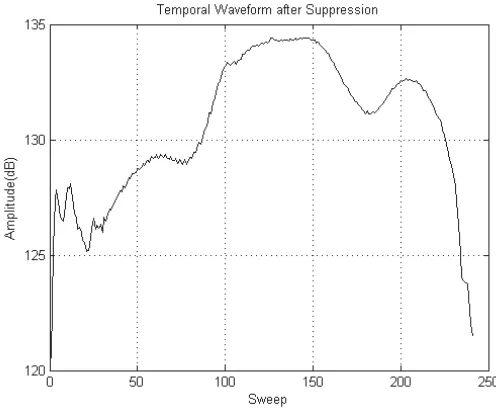
Figure 1 shows the original temporal waveform of the first group which is corresponding to a certain azimuth-range cell. As can be seen, the dominant waveform energy is produced by the low-frequency clutter, vibrating slowly and slightly, whereas the target signal modulated on clutter waveform is weak when compared with clutter amplitude, vibrating severely. The solid line in Fig. 3 shows its Doppler spectrum with IMI unsuppressed, where the dominant energy is concentrated to the center frequency, exhibited as the clutter components, and a target peak shown at about −0.34 Hz. Here, the X-axis denotes the normalized frequency, that is, the true frequency divided by the A/D sample frequency.
has disappeared in the remaining temporal waveform as illustrated in Fig. 2.
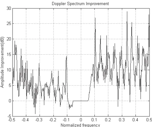
When comparing the Doppler spectrums of suppressed and unsuppressed, as shown in Fig. 3, we can see that the noise floor has been dropped down for about 10 dB after suppression by means of this proposed algorithm. However, this processing brings a little impact on the true target peak at −0.34 Hz. Another attractive merit is that it does not change amplitudes in low frequency band, mainly corresponding to Bragg peaks or ground clutter. Few reported algorithms have this advantage of no impact on clutter. But a disadvantage is that when the target falls in the low frequency segment surrounding the clutter, this proposed algorithm brings no processing gains or improvement on the noise floor or SNR, either negative or positive gains. The target peak at near clutter will remain unchanged. Detailed Doppler spectrum improvements for Fig. 3 is illustrated in Fig. 4. The improvement above 0 dB means the suppressed spectrum is lower than that of unsuppressed at a certain Doppler bin, leading to an expected improvement on floor falling. This figure highlights a fact that the floor has been dropped down significantly, with the maximum improvement about 28 dB and the mean 7.1725 dB through accurate calculation. Furthermore, at the low frequency section, there is no change, namely 0 dB improvement.
As can be seen, the processed temporal waveform exhibits an unexpected vibration on the low sweep (0–20 sweeps). The amplitude vibration may be caused by the projection. At the border or the edge, the continuity of signal is broken. When we perform DFT or FFT, we implicitly perform a periodic expanding of this finite segment of signal into an infinite periodic series signal. So the discontinuity at the border of every period segment is obvious, which may be regarded as an unexpected false IMI. Or this discontinuity exhibits as an IMI. Projection will “smooth” this discontinuity.
Figure 1. Original temporal waveform.
Figure 3. Doppler spectrum comparison.
Figure 5. Doppler spectrum comparison.
proves that this projection algorithm has perfect performance for IMI suppression while brings little impact on the true target signal.
Detailed Doppler spectrum improvements for Fig. 5 are illustrated in Fig. 6. This figure shows its improvement with the maximum about 36 dB and the mean 12.177 dB through accurate calculation, and no change at the low frequency section.
5. CONCLUSION
A viable algorithm for temporal IMI suppression for OTHR has been developed and demonstrated in this paper, where we exploit the fact that the IMI phase spectrum can be regarded as complex cosine. After clutter suppression, this cosine signal exhibits as a strong pseudo-target. Therefore, subspace analysis and projection can be used here to filter out the IMI as a pseudo-target. Experimental data from real OTHR system are used to verify its performance. Consequently, this proposed algorithm can work soundly and efficiently. This proposed algorithm has the following advantages:
1) Directly use the Doppler data from coherent integration, without extra DFT or IDFT;
2) No impact on clutter such as clutter peak expanding; 3) A little impact on true target peak;
4) Only need a rather simple clutter suppression.
5) Neither require nor estimate the temporal position of IMI.
REFERENCES
1. Headrick, J. M. and M. I. Skolnik, “Over-the-horizon radar in the HF band,”Proceedings of the IEEE, Vol. 62, No. 6, 664–673, Jun. 1974.
2. Maresca, J., Jr. and J. Barnum, “Theoretical limitation of the sea on the detection of low Doppler targets by over-the-horizon radar,”
IEEE Transactions on Antennas and Propagation, Vol. 30, 837– 845, Sept. 1982.
3. Gill, E., et al., “The effect of bistatic scattering angle on the high frequency radar cross sections of the ocean surface,” IEEE Geoscience and Remote Sensing Letters, Vol. 5, No. 2, 143–146, 2008.
5. Khan, R. H., et al., “Experimental results from a long-range HF ground wave coastal surveillance radar,” IEEE National Radar Conference, 20–22, Boston, USA, May 20, 1993.
6. Bazin, V., et al., “Nostradamus: An OTH radar,”IEEE Aerospace and Electronic Systems Magazine, Vol. 21, 3–11, 2006.
7. Fabrizio, G. A., A. B. Gershman, and M. D. Turley, “Non-stationary interference cancellation in HF surface wave radar,”
Proceedings of the International Radar Conference 2003, 672–677, Sept. 3–5, 2003.
8. Fabrizio, G. A., A. B. Gershman, and M. D. Turley, “Robust adaptive beamforming for HF surface wave over-the-horizon radar,”IEEE Trans. on AES, Vol. 40, 510–525, Apr. 2004. 9. Wei, M., et al., “Meteor trail interference model in HF
environment,”2006 International Conference on Communication, Circuits and Systems Proceedings, 624–628, Jun. 25, 2006. 10. Liu, T., et al., “Fractal features and detection of meteor
interference in OTHR,” 2006 CIE International Conference on Radar, 1–5, Shanghai, China, Oct. 16–19, 2006.
11. Liu, T., et al., “An effective fractal algorithm for meteor interference detection in OTHR,” 2006 China-Japan Joint
Microwave Conference Proceeding, 727–731, Chengdu, China,
2006.
12. Barnum, J. R. and E. E. Simpson, “Over-the-horizon radar sensitivity enhancement by impulsive noise excision,” IEEE National Radar Conferernce, 252–256, 1997.
13. Khan, R. H., “Ocean-clutter model for high-frequency radar,”
IEEE Journal of Oceanic Engineering, Vol. 16, 181–188, 1991. 14. Guo, X., et al., “Development of sky wave over-the-horizon radar,”
ACTA Aeronautica et Astronautica Sinica, Vol. 23, 495–500, 2002. 15. Turley, M., “Impulsive noise rejection in HF radar using a linear prediction technique,” Proceedings of the International Radar Conference, 358–362, Sept. 3–5, 2003.
16. Fabrizio, G. A., A. Farina, and M. D. Turley, “Spatial adaptive subspace detection in OTH radar,”IEEE Trans. on AES, Vol. 39, 1407–1428, Oct. 2003.
17. Fabrizio, G. A., D. A. Gray, and M. D. Turley, “Parametric localisation of space-time distributed sources,” 2000 IEEE
International Conference on Acoustics, Speech, and Signal
Processing, Vol. 5, 3097–3100, 2000.
Proceedings, Vol. 4, 1033–1036, Toulouse, May 14–19, 2006. 19. Huang, L., et al., “Suppressing instantaneous interference of high
frequency ground wave radar,”Chinese Journal of Radio Science, Vol. 19, 166–170, 2004.
20. Xing, M.-D., et al., “Transient interference excision in OTHR,”
Acta Electronica Sinica, Vol. 30, 823–826, 2002.
21. Root, B., “HF radar ship detection through clutter cancellation,”
Proceedings of the 1998 IEEE Radar Conference, 281–286,
May 11–14, 1998.
22. Horn, R. A.,Matrix Analysis, Cambridge University Press, 1990. 23. Guo, X., H. Sun, and T. S. Yeo, “Interference cancellation for high-frequency surface wave radar,”IEEE Trans. on Geoscience and Remote Sensing, Vol. 46, 1879–1891, Jul. 2008.
24. Guo, X., H. Sun, and T. S. Yeo, “Transient interference excision in over-the-horizon radar using adaptive time-frequency analysis,”
IEEE Trans. on Geoscience and Remote Sensing, Vol. 43, 722–
735, Apr. 2005.
25. Fabrizio, G. A., “Over the horizon radar,” IEEE Radar Conference, 1–2, May 26–30, 2008.
26. Holdsworth, D. A. and G. A. Fabrizio, “HF interference mitigation using STAP with dynamic degrees of freedom allocation,” 2008 International Conference on Radar, 317–322, Sept. 2–5, 2008. 27. Liu, T., J. Wang, and Y. Gong, “OTHR impulsive interference
detection based on AR model in phase domain,”WSEAS Trans. on Signal Processing, adopted.
28. Golub, G. H. and C. F. Van Loan, Matrix Computations, 3rd Edition, The Johns Hopkins University Press, Baltimore and London, 1996.