All Loop Topological String Amplitudes
from Chern-Simons Theory
The Harvard community has made this
article openly available.
Please share
how
this access benefits you. Your story matters
Citation Aganagic, Mina, Marcos Mariño, and Cumrun Vafa. 2004. “All Loop Topological String Amplitudes from Chern-Simons Theory.” Communications in Mathematical Physics 247 (2): 467–512. https:// doi.org/10.1007/s00220-004-1067-x.
Citable link http://nrs.harvard.edu/urn-3:HUL.InstRepos:41384996
Terms of Use This article was downloaded from Harvard University’s DASH repository, and is made available under the terms and conditions applicable to Other Posted Material, as set forth at http://
arXiv:hep-th/0206164v1 18 Jun 2002
HUTP-02/A024 hep-th/0206164
All Loop Topological String Amplitudes
From Chern-Simons Theory
Mina Aganagic, Marcos Mari˜no and Cumrun Vafa
Jefferson Physical Laboratory Harvard University Cambridge, MA 02138, USA
Abstract
We demonstrate the equivalence of all loop closed topological string amplitudes on toric local Calabi-Yau threefolds with computations of certain knot invariants for Chern-Simons theory. We use this equivalence to compute the topological string amplitudes in certain cases to very high degree and to all genera. In particular we explicitly compute the topological string amplitudes for IP2 up to degree 12 and IP1 ×IP1 up to total degree 10 to all genera. This also leads to certain novel large N dualities in the context of ordinary superstrings, involving duals of type II superstrings on local Calabi-Yau three-folds without any fluxes.
1. Introduction
In [1] it was conjectured that U(N) Chern-Simons theory on S3, which describes topological A-model ofN D-branes onX =T∗S3, is dual at large N to topological closed string theory on Xt = O(−1) ⊕ O(−1) → IP1. There it was shown that the ’t Hooft expansion of Chern-Simons free energy agrees with topological string amplitudes on Xt to all genera. The conjecture was further tested in [2], where computations of certain Wilson loop observables in Chern-Simons theory were shown to match the corresponding
quantities on Xt. Various aspects of the duality were studied in [3,4,5,6,7,8,9,10] from different points of view. The topological string duality was embedded in the superstring theory in [11]. In [12] the target space derivation of the superstring duality of [11] was found by lifting up to M-theory [12,13]. This was further studied in [14,15], and also in a related context in [16,17,18,19,20,21,22,23]. Recently, [24] gave a world-sheet proof of the topological string duality based on some earlier ideas in [1].
In [25] a large class of new large N dualities was proposed which generalize the
con-jecture of [1] to more general backgrounds, employing the philosophy of [1] that the large
N dualities are geometric transitions. On the open string side, replacing T∗S3 with a more general Calabi-Yau manifold X led one to incorporate large open string instantons whose contributions deform Chern-Simons theory [26]. In the spirit of ’t Hooft’s original large N conjecture, the holes in open string Riemann surfaces fill up at large N, and the complicated open string instanton sums that arise in a general Calabi-Yau X get related to a complicated structure of instantons on the dual closed string side. Some important aspects of how this works were clarified in [27]. For one of the examples of [25], where both
sides of the duality are explicitly computable to all orders [27] verifies the correspondence at the level of the partition functions. However, in a general setting, the descriptions of
the theory in terms of open and closed strings are at the same level of complexity, and the duality was not easy to check (beyond the leading disk amplitude).
In this paper, by combining all of the ideas above together with several new technical ingredients, we show that Chern-Simons theory with product gauge groups and topological matter in bifundamental representations computes all loop topological string amplitudes on non-compact toric Calabi-Yau manifolds. Namely, it is shown that open string duals of
with knots that are the boundaries of the annuli. The duality is local in the sense that, as in [1], the three-manifolds wrapped by D-branes get replaced by IP1’s in the dual. However in this case, open string theories build very complicated closed string geometries: in fact
any noncompact toric Calabi-Yau manifold arises in some limit of this.
The paper is organized as follows. In section 2 we review the relevant geometries
for open and closed strings that are related by large N duality. In section 3, we discuss
the physics of open string theories, and explain why the model simplifies dramatically
using a deformation argument. In section 4 we explain what is the relevant Chern-Simons
computation in terms of three-manifolds glued with annuli. In section 5 we propose the
largeN dualities and we argue that the results of [24] should be applicable to derive them. In section 6 we discuss the relation between the predictions of this duality to localization in
the A-model closed string computation. In section 7 we present explicit evaluations of the
amplitudes and provide predictions for the integer invariants for some examples including
IP2 and IP1 × IP1, and we show that they agree with the known results when they are available [28][29][30][31]. In section 8 we consider embedding of this in the superstring
context. Results of previous sections give open string duals of closed string geometries
with no RR flux. Moreover, we show that some local geometries in IIB string theory have
dual description in terms of gauge theory alone.
The work in section 7.2. was done in collaboration with P. Ramadevi, to whom we are very grateful. Also, our work has some overlap with the work of [32], and we thank
the authors for discussing their work prior to publication. In particular we learned of their
result that only a limited number of holomorphic curves contributes to the amplitudes
before we found the general argument presented in section 3. The argument discussed in
[32] (in the context of dP2) uses localization principle, whereas our argument that only annuli contribute for all toric 3-folds is based on complex structure deformation invariance.
2. Geometry
2.1. Open String Geometry: T2 Fibrations and Their Degenerations
In this paper, the relevant Calabi-Yau manifolds are non-compact and admit a
in IR3 that correspond to the discriminant of the fibration. A very familiar example of a Calabi-Yau manifold of this type is X =T∗S3. The complex structure of X is given by
xy=z, uv =z+µ, (2.1)
The two-torus is visible in the above equation as it is generated by two U(1) isometries of
X acting as
x, y, u, v →xeiα, ye−iα, ueiβ, ve−iβ.
The α and β actions above can be taken to generate the (1,0) and (0,1) cycle of the T2. The local type of the singularity has a T2 fiber that degenerates to S1 by collapsing one of its one-cycles. In the equation above, theU(1)α action fixesx= 0 =yand therefore fails to generate a circle there. In the total space, the locus where this happens, i.e. the
x = 0 = y = z subspace of X, is another cylinder uv = µ. The projection to the base space forgets the circle of this cylinder and is a line in IR3.
Such a geometry locally looks like a Taub-Nut (TN) space times a cylinder C∗ = IR×S1. Here, the TN space itself is thought of as a cylinder xy = const which is fibered over the z plane and which degenerates at z = 0. Analogous considerations apply to the
U(1)β action. The locus of degenerate fibers in the base IR3 of the deformed conifold is given in the figure below. In this and similar figures below, two of the directions of the base are the axes of the two cylinders, and the third direction represents the real axis of the z−plane.
α
β
re(z)
Fig. 1The figure depicts the discriminant locus of the T2
×IR fibration in the base IR3
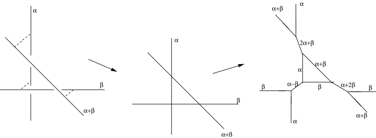
[image:5.612.163.454.490.662.2]In general, any (p, q) cycle of the T2 can degenerate in this way. As long as the de-generate loci do not intersect, the local geometry is that of Taub-Nut space, as an SL(2,Z) transformation on the T2 fiber can be used to relate it to the degenerations discussed above. In what follows, it will be important that the orientation of the locus where theT2 fiber degenerates in the base IR3 is correlated with the (p, q) type of degenerating cycle. We have seen an example of this above in the case of T∗S3, where the α and β cycles degen-erated along orthogonal directions in the base in fig. 1. The origin of this is the fact that the Calabi-Yau manifold is a complex manifold and the fibration is special Lagrangian.
We will not go into detail here in this language as it is cumbersome for physicists, and explained in the literature (see for example [25])1, especially because there is a string theory duality that provides excellent intuition about the geometry, which we would like to explain instead.
α
β
α+β
Fig. 2The degeneration locus of theT2
fibration in the base specifies the Calabi-Yau geometry. The orientation of the lines are related to the (p, q) type of the 1-cycle that degenerates over it. In the type IIB language, this corresponds to different (p, q) fivebranes.
1 To give an idea of the more general situation, let ˆx
α,β be the single valued holomorphic
coordinates onC∗×C∗, and letz be a coordinate on IR2
. If a (p, q) cycle of the T2 degenerates at a point in z, then the fixed point locus which is invariant under ˆxα→xˆαeipθ,xˆβ →xˆβeiqθ. In
terms of periodic variables ˆxα,β = exp(xα,β) we can write the degeneration locus as by
[image:6.612.201.412.312.494.2]2.2. Relation to (p, q) Fivebranes in IIB
In this section we connect the description of Calabi-Yau geometry by a duality to the web of (p, q) fivebranes [33]. This will be helpful for us for an intuitive picture of holomorphic curves in the geometry. The connection was derived in [34] and we will now review it.
Recall that M-theory on T2 is related to type IIB string theory on S1. Since the Calabi-Yau manifolds we have been considering areT2 fibered over B= IR4, we can relate geometric M theory compactification on Calabi-Yau manifold X to type IIB on flat space on B×S1. However, due to the fact that T2 is not fibered trivially, this is not related to the vacuum type IIB compactification.
The local type of singularity, as we have seen above, is the Taub Nut space T Np,q, where the (p, q) label denotes which cycle of theT2 corresponds to theS1 of the Taub-Nut geometry. Under the duality, this local degeneration of X is mapped to the (p, q) five-brane that wraps the discriminant locus in the base space B, and lives on a point on the
S1. The fact that the (p, q) type of the five brane is correlated with its orientation in the base is a consequence of the BPS condition. More precisely, configurations of five branes that preserve supersymmetry and 4 + 1-dimensional Lorentz invariance are pointlike in a fixed IR2 subspace of the base that we called the z plane above. In the two remaining directions of the base, the five branes are lines where the equation of the (p, q) five brane is pxα+qxβ = const.
2.3. Geometric Transitions
Consider a pair of lines in the base space over which two one-cycles of the T2 degen-erate. Any path in the base space ending on the two lines, together with the T2 fiber over it, gives rise to a closed three-manifold in the total space. This is because a cycle of the
T2 degenerates over the start and the end point of the path, so the three-manifold has no boundaries. If the two lines intersect in the base space, the three-cycle obtained in this way can be shrunken to a point. If they don’t, it generates a homology class inH3(X,Z). Let n be the number of five-branes. If the five branes are in generic positions and do not intersect, the manifold is smooth, and it is easy to see that the the dimension of third homology is b3(X) =n−1.
D-branes wrapped on them preserve some supersymmetry of the theory. These cycles are
volume-minimizing and project to paths of shortest length in the base (the Lagrangian
condition can always be satisfied with some choice of symplectic form on X). In the
non-compact situation we are discussing, the meaning of this is particularly transparent
in the IIB string theory as the five-branes live in IR4 with flat metric. The number of supersymmetric cycles, for five-branes in generic positions, is easily counted by doing the
projection of the base IR3 → IR2 that suppresses the z-direction and counts the number of intersections. Generically there will be n(n−1)/2 such intersection points (unless some
(p, q) 5-branes are of the same type).
The Calabi-Yau manifolds we have been discussing have geometric transitions where
three-cycles in geometry shrink and the resulting singularity is smoothed to a manifold
Xt of different topology. This was explained in some detail in [25]. In the examples we
will be studying in this paper, the local geometry of the singularity will be T∗S3, so the geometric transition in question involves anS3shrinking and a IP1 growing. The geometric transitions do not spoil the fact that the manifold is T2 fibered, however they do change the locus of singular fibers. After the transition that shrinks all the three-cycles (and these
always exist in the family of X’s we consider), the resulting manifolds are toric varieties.
Toric varieties admit a group of U(1) isometries whose rank is the complex dimension
of the manifold. In our case this is U(1)3, and the symmetry enhancement comes from the fact that the transition which gets rid of all the three-cycles requires all the loci of
singular fibers to coincide in the z-plane, and the extra U(1) is the group of rotations
about this point. While the reader might get an impression from the above discussion that
the manifold after transition gains new cycles only in H2(Xt,Z), this is in fact not the case. In fact, in the generic case the number of shrinking minimal three-cycles is larger
than the number of classes in H3(X). Then, since not all three-cycles are independent in homology, there are four-chains with boundaries on some of them corresponding to the
relations which they satisfy. After the transition, the four-chains close off because their
boundaries shrink. As a consequence, the dual geometry does involve compact cycles in
α+β β α
β
α+β
α α+β α
α+β α
α
β α−β β β
2α+β
α+β
α+2β
Fig. 3This shows the geometric transition of the Calabi-Yau in the previous figure. In the leftmost geometry there are three minimal 3-cycles. The lengths of the dashed lines are proportional to their sizes. The intermediate geometry is singular, and the figure on the right is the base of the smooth toric Calabi-Yau after the transition. This Calabi-Yau is related to IB3 by flopping three IP
1
’s.
In the language of (p, q) five branes, the geometric transition corresponds to a phase transition in the five-dimensional theory. Namely, the configuration of intersecting (1,0) and (0,1) five-branes is a phase transition point: the Higgs phase with five-branes sepa-rated in the z plane2 meets the Coulomb phase, where a piece of (1,1) brane resolves the singularity. In the geometry, there is a T2 fiber whose (1,1) cycle degenerates over this interval, and the cylinder is capped off to a IP1 by all the cycles of the T2 degenerating over the boundaries of the interval. The singularity can also be resolved with a (1,−1) brane, which corresponds to the flopped IP1.
2.4. Geometry of Holomorphic Curves
Calabi-Yau manifolds generally come with families of embedded curves. In the topo-logical A-model only holomorphic curves are relevant, as the A-model string amplitudes localize on them. In the presence of D-branes wrapping Lagrangian submanifolds Mi in
X, we must also consider holomorphic curves with boundaries on the Mi’s.
Holomorphic curves have a very simple description in the toric base, or equivalently, in the (p, q) five brane language. Let us first consider closed string geometries, the family
2 Recall that this is the complex structure modulus of the geometry. The five dimensional
[image:9.612.117.503.69.211.2]of Calabi-Yau manifolds we have calledXt above. In this case, it can be shown that all the compact holomorphic curves in a non-compact toric Calabi-Yau manifold wrap a 1-cycle in theT2 fiber direction. Holomorphic curves project to lines in the toric base, and locally the direction of the curve in the base is correlated with its direction in the fiber. For the compact curves, the direction in the fiber is the (p, q) 1-cycle of the T2. This is most transparent in the (p, q) five-brane language.
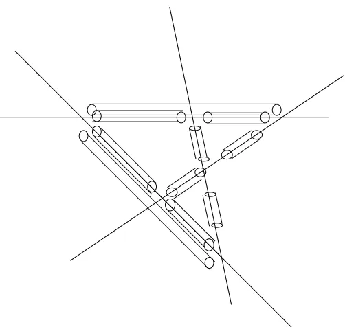
Fig. 4The figure on the left depicts a genus one holomorphic curve with three holes ending on three minimal three-cycles. The figure on the right is after the transition, and also depicts a genus one curve, but without boundaries.
Namely, consider an M-theory membrane, wrapping a holomorphic curve on Xt. By
M-theory/type IIB duality, a membrane wrapping a (p, q) cycle of theT2 is dual to a (p, q) string, therefore membranes on holomorphic curves in Xt that are along the T2 in the fiber are dual to webs of (p, q) strings in type IIB string theory that are BPS. Moreover, the compact curves are related to webs ending on (p, q) five-branes [33]. An example of such a curve is given in the right portion of fig. 4.
[image:10.612.145.468.201.346.2]generic locations in thez plane, the string webs are never compact. This situation changes if strings can end elsewhere. For example, if there are M-theory five-branes wrapped on Lagrangian cycles inX, membranes can end on them. The M-theory five-brane is replaced with a D3-brane in IIB string theory ending on the various (p, q) five-branes. There are then compact string webs ending on the D3-branes, corresponding to holomorphic curves with boundaries. In relation to large N dualities in superstring context it is more natural to consider type IIA string on X instead, with D6-branes on the Mi’s. This is related, via duality of IIA/M-theory on S1, to IIB string theory with Kaluza-Klein monopoles ending on the (p, q) five brane web [7]. Namely, the D6 branes in Lagrangian submanifolds of
X lift to M-theory on a G2 holonomy manifold. To obtain this manifold, we need to consider an extra S1 which is fibered over the corresponding CY. This is related to IIB on
B×S1 where we exchange the 11-th circle with the T2 that fibers X. What used to be the 11-th circle is now fibered nontrivially over B. In particular, the circle vanishes over a 2-dimensional subspace of the type IIB 5-dimensional geometry. It vanishes along the line in B ending on the (p, q) five branes as well as on the S1 which is dual to the T2 of M-theory. This line in B corresponds to the line in the base ofX over which there is the three-manifold that the D6 brane wraps. The IIB 5-brane web is in a background of ALF geometry dictated by the location of the Lagrangian submanifold inX.
2.5. Geometry of Three-Cycles
In this paper, we will wrap D-branes on the minimal three-manifolds in X. The physics of the D-branes depends on both X and the three-manifold M it is wrapped on, so we will describe the geometries of the latter.
In our context,M is obtained by pinching the cycles of theT2fibers over the endpoints of an interval in the base. Clearly, if the same cycle vanishes at both ends, the topology of the three-manifold is S2×S1, as there is a cycle of the T2 that never vanishes on M. An example where the manifold is S3 arises in the familiar context of T∗S3. This S3 comes from a (1,0) cycle of the T2 vanishing at one end, and (0,1) cycle vanishing on the other. To see that this is anS3, note that at x= ¯y andu =−¯v the equation (2.1) definingT∗S3 becomes
|x|2+|u|2=µ,
the phase of x = ¯y, degenerating at the end with x = 0, and the (0,1) cycle that is the phase of u= −v¯ degenerating over the u= 0 endpoint 3.
More generally, we have the following. For our current purpose, by an SL(2,Z) trans-formation of the T2 we can make (1,0) be the vanishing cycle over one of the boundaries, and let (q, p) be the cycle that vanish over the other. The 3−manifold itself is a Lens space
L(p, q). Remember that lens spaces are defined as quotients of S3 by a Zp action. The space L(p, q) is given by
|x|2+|u|2 = 1 (x, u)∼(exp(2iπ/p)x,exp(2iπq/p)u). (2.2) To see that, consider an S3 which, as explained above, is a T2 fibration over an interval, where the cycles of theT2 are generated by phases of x, u. If the complex structure of the
T2 corresponding to S3 it is τ, then an SL(2,Z) transformation that takes this T2 to a
T2 with (1,0) and (q, p) cycles vanishing over the endpoints will take τ to τ′ = τ+pq. But the T2 with the new complex structure is precisely a quotient of the original one by the Zp action specified in (2.2). Note that L(p, q) is homeomorphic to L(p,1). In the present
context this corresponds to the fact that global SL(2,Z) transformations preserving the
(1,0) cycle of the T2 can be used to set q to one.
For our later considerations in this paper it is important to have another view on
this construction of a three-manifold M as a T2 fiber over interval. The construction is as follows: we are gluing two solid tori over (say) the midpoint of the interval, up to an
SL(2,Z) transformation VM that corresponds to a diffeomorphism identification of their boundaries. Let us call the two tori on each side of the midpoint by T2
L and TR2. The embedding of this in the Calabi-Yau geometry provides a canonical choice of VM. In the Calabi-Yau geometry, there is a natural choice of basis of cycles α, β of the T2 that fibers X, which is provided by the choice of complex structure on X. We can identify the one-cycles of the T2 fiber that shrink over the left and the right sides of the interval with the shrinking 1-cycles of TL and TR. The diffeomorphism map VM is the SL(2,Z) transformation that relates one of the shrinking cycles of the fiber of X to the other one.
Let us now explain the construction of the gluing matrices that will suit our purpose.
Let (pL, qL) be the cycle of theT2 fiber that degenerates over the left half onM, and let 3 This is in fact the minimalS3
(pR, qR) be the cycle that degenerates over the right half. The gluing matrix VM can be written as
VM =VL−1VR, (2.3)
where VL,R =
pL,R sL,R
qL,R tL,R
∈ SL(2,Z) Clearly, VM is unique up to a homeomorphism
that changes the “framing” of three-manifold [36] and takes
VL,R →VL,R TnL,R
where T is a generator of SL(2,Z), T =
1 1 0 1
. This is a consequence of the fact that
there is no natural choice of the cycle that is finite on the solid torus.
In the case of M =S3 above, since (1,0) degenerates in the left half of M and (0,1) in the right half, VM =S, where S=
0 −1 1 0
. As a small modification, we could make
(p,1) degenerate over the left half instead, so that VL =TpS is a lens space L(p,1) and V isS−1T−pS. For most considerations in this paper we will be considering the casesL(1,1) or L(1,0), which are homeomorphic to S3.
3. Open String Theory
We are interested in the topological A-model on the Calabi-Yau geometries described above, with D-branes wrapping special Lagrangian three-spheres. The local geometry in some neighborhood of a Lagrangian three-manifold M is T∗M and it was shown in [26] that the topological A-model corresponding toN D-branes onM is a U(N) Chern-Simons theory on three-manifold M,
Z =
Z
DAeSCS(A)
where
SCS(A) =
ik
4π
Z
M
Tr(A∧dA+ 2
3A∧A∧A)
is the Chern-Simons action. The basic idea of this equivalence is as follows: the path-integral of the topological A-model localizes on holomorphic curves. When there are D-branes, this means holomorphic curves with boundaries ending on them. In the T∗M
field theory formulation demonstrates [37]). In this map, the level k would be naively
related to the inverse of the string coupling constant gs. However, quantum corrections
[36] shift this identification to
2πi
k+N =gs.
More globally, however, the geometry is generally not that of the cotangent space to
any manifold, and there can be D-branes wrapping other minimal three-spheres in X. In
this case the topological open strings will have contributions from degenerate holomorphic
curves, which are captured by Chern-Simons theories, as well as some honest holomorphic
curves, which lead to insertion of some Wilson loop observables for the Chern-Simons
theory [26]. If we have a number ofMi’s distributed in some way inside a Calabi-Yau, with
Ni D-branes wrapped over Mi, then we can trade the degenerate holomorphic curves by
including the corresponding Chern-Simons theoriesSi =SCS(Ai) coupled in an appropriate way with the honest holomorphic curves. Namely, we have
eFall =Z Y
i
DAieSi+Fndg(Ui(γi)) (3.1)
where Fall denotes the full topological A-model amplitude, and Fndg denotes the contri-bution of the non-degenerate holomorphic curves to the topological amplitudes. These
holomorphic curves give rise to Wilson loops on the D-branes: each holomorphic curve
with area A ending on Mi over the knot γi leads to the contribution e−AQiTrUi(γi) to
Fndg, where Ui(γi) denotes the holonomy of the Chern-Simons gauge connection around the knotγi. Notice that all these Chern-Simons theories have the same coupling constant.
More precisely,
2πi ki+Ni
=gs
In the toric examples we will consider in this paper it turns out that only holomorphic
annuli contribute to Fndg and thus this connection with Chern-Simons theory is a useful way to compute the topological A-model amplitudes as some particular correlation function
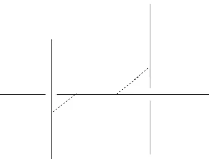
Fig. 5Calabi-Yau geometry withb2= 1, b3= 2and two minimalS 3
’s as the dashed lines.
3.1. The Annulus Amplitude
As an example, let us consider the Calabi-Yau manifold X with b3 = 2, b2 = 1 in fig. 5, whose complex structure is described by
xy= z
x′y′= (z−µ1)(z−µ2).
(3.2)
and was studied in a physics context in [38]. In X, the α cycle of the T2 degenerates over the point z = 0, but the β cycle degenerates twice, over z = µ1 and µ2. The cycles over [µ1,0] and [0, µ2] are three–spheresM1,2 that generateH3(X) . The base space ofX, with loci with degenerate fibers – is pictured in fig. 5, where we have taken µ’s to be real, and
µ1 < 0 < µ2 (the reader should keep in mind that only one of the dimensions of the z plane is visible in the base).
As is clear from the picture, there is an additional parameter visible in the base: the relative distance of two β-branes. This is a K¨ahler parameter corresponding to the one compact 2-cycle in X (since X contains an S2 ×S1, as we discussed above, it certainly contains an S2 that cannot be contracted – we simply pick a point on the S1 in S2 ×S1) 4.
4 The interpretation of this K¨ahler parameter is obvious in the type IIB dual, as it is the
scalar field of the six dimensional N = (1,1) supersymmetric theory on the two parallel (0,1) five-branes. Duality relates this to a Calabi-Yau three-fold in M-theory containing a curve of A1
[image:15.612.201.413.69.231.2]As we discussed above, at the level of topological strings the theory is aU(N1)×U(N2) Chern-Simons theory, but since there are two stacks of D-branes, there is a new open string
sector where one end of the string is on the D-branes wrapping M1 and the other on M2. The ground states of this string correspond to constant maps to the S1 that the three-manifolds “intersect” over. Correspondingly, there are two states in the Ramond sector
of the topological string, a real scalar and a one form, with U(1)R charges −1/2 and 1/2.
Only the scalar is physical, and taking into account both orientations of the string, we get
a complex scalar φ in (N1, N2). This complex scalar is generically massive, and its mass is proportional to the “distance” between M1 and M2 given by the complexified K¨ahler parameter r. We will show below that the only modification of the topological string we
need to make in this geometry is to include the minimally coupled complex scalar in this
sector. Because of the topological invariance of the theory the action of a charged scalar
with minimal coupling is of the form Lφ∼ Hγ Tr ¯φ(d−A1 +A2)φ. Note that the scalar field gets a mass from turning on a Wilson line on theS1 it propagates on. We will pick its “background” value which we denote byrbelow. The path integral involvingφis Gaussian
so it can be easily evaluated [2] and gives:
O(U1, U2;r) = exp
h
−Tr log(er/2U1−1/2⊗U21/2−e−r/2U11/2⊗U2−1/2)i = expn
∞
X
n=1 e−nr
n TrU
n
1 TrU2−n
o
,
(3.3)
where U1,2 are the holonomies of the corresponding gauge fields around a loop 5
Ui = P exp
I
γ
Ai ∈U(Ni), i = 1,2.
5 In going from the first to the second line in (3.3), we have dropped a factor of det(U1/2 1 )det(U
−1/2 2 )
in O. This factor, which equals exp(
√
N1
2
H
γTrA1−
√
N2
2
H
γTrA2), can be absorbed away in a
redefinition ofr. It is likely that this is related to the holomorphic anomaly of topological strings
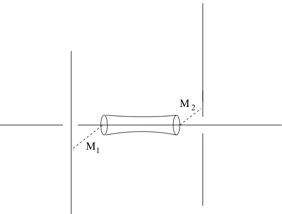
M1
M2
Fig. 6There is one holomorphic annulus connecting the twoS3
’s. This corresponds to a one-loop computation with a bifundamental string running around the loop.
Note that the operator O is the amplitude for a primitive annulus of size r with
boundaries on M1 andM2, together with its multicovers [2][5][8]. This annulus is depicted in fig. 6, and it is a piece of the holomorphic curve that is wrapped by the (1,0) brane.
This curve is obtained by setting x = 0 =y =z in (3.2) and is given by x′y′ =µ1µ2. The Chern-Simons path integral in this geometry is therefore defined with the
inser-tion of the above operator. The path integral of the A-model string field theory in this
background is therefore given by:
Z =
Z
DA1DA2eSCS(A1)+SCS(A2)exp
n
−
∞
X
n=1 e−nr
n TrU
n
1TrU2−n
o
(3.4)
To recapitulate, we have Chern Simons theory on two three-manifolds M1 and M2 con-nected via an annulus. The boundaries of the annulus look like S1’s in both of them, i.e. we have one knot in each Mi. The topological theory is computing the expectation value
of the operator O(U1, U2;r), which involves Wilson loop operators around the two knots. This obviously extends to more general configurations: for every pair of three-manifolds
M1 and M2 that are connected by a holomorphic annulus, we will get a bifundamental complex scalar. Integrating this field out, we find we need to insert an operator (3.3),
[image:17.612.164.449.70.286.2]M
M
1
2 M3
Fig. 7In the left figure, it looks like there is a family of holomorphic annuli between M1 and M2, and a holomorphic annulus connecting M1 with M3. However, by
moving in the complex structure moduli space we get to the figure in the right, where it is clear that there is an isolated holomorphic annulus connecting M1 and
M2 and no holomorphic curve between M1 and M3.
As an example, consider fig. 7. There are Ni D-branes wrapping a chain of four
minimal spheres Mi, i = 1, . . .4 connecting two (1,0) branes and two (0,1) branes. For every pair of spheres intersecting over an S1 we get a bifundamental scalar field, so we have matter in representations (Ni, Ni+1), where i = 5 corresponds to the first sphere again. Note that in the (N1, N2) and (N3, N4) sector, the bifundamental scalar is not localized, and correspondingly in fig. 7 there is a family of annuli. In fact, a careful reader has probably noticed that this could have happened in the two-sphere case as well, had we not chosen judiciously the ordering of (1,0) and (0,1) branes in the z direction of the base. In other words, we could have picked µ1, µ2 >0 in (3.2) , and we would have found a family of annuli. See fig. 7. This objection is in fact its own cure. Namely, by changing the complex structure of X we could go from one configuration to the other. In fact, using the other direction in the z-plane we can do this in a smooth way, as the µ’s are
complex, without passing through a singularity of the three manifold. On the other hand, the topological A-model amplitudes cannot depend on the complex structure moduli. As a consequence, the value of operators O(Ui, Ui+1;ri) cannot change in passing between the two configurations, and they are given by the annulus computation we already outlined.
This idea is rather powerful and it leads to the fact that, in all the toric cases, the only holomorphic curves are annuli connecting pairs of S3’s along lines on the toric base (i.e. along loci of (p, q) 5-branes). The argument for this is extremely simple: as we
[image:18.612.127.488.69.222.2]moduli space, where it is manifest that the only holomorphic curves are annuli. By the fact that topological A-model amplitudes do not depend on complex structure moduli, we can immediately conclude that only annuli contribute to topological string amplitudes. Let us now explain why this preserves only annuli. At a generic point of the complex structure moduli space (which we can always choose), the T2 fibers degenerate over a set of points in the z plane, and the three-cycles Mi in X project to lines connecting them, which are generically not aligned. Recall that the holomorphic curves project to points in thez plane. This means that the “large” holomorphic curves must project to points in the
z-plane (as discussed in section 2) where different Mi’s intersect, and for a generic choice of complex structure these are the points where theT2 fibers degenerate. In other words, we are left only with annuli over loci where the T2 fibration degenerates, as we wished to show6.
4. D-branes on Chains of Three-Manifolds and Knot Invariants
In order to evaluate the A-model partition functions in these backgrounds we need a few additional pieces of data. Namely, we need to know how the different knots are linked, in particular their linking numbers lk(γi, γj), and also what is their framing – the self linking number of each of γi’s. As it is explained in [36][40], the framing is a rather subtle effect from the point of view of Chern-Simons theory, having to do with the fact that in evaluating expectation values of Wilson loop operator associated to the knot, one encounters certain ambiguities in the calculation. These are akin to a choice of point-splitting regularisation, since to calculate the self-linking number in a way that is consistent with topological invariance one must choose a “framing” by thickening a knot into a ribbon. Different framings differ by adding twists to the ribbon, the framing itself being defined as the linking number of the two edges of the ribbon. The Wilson loop operators are not invariant under the change of framing. We will show below that different choices of framing correspond in the present context to different target space geometries. The role of framing in topological string theory was discovered in [7] in a closely related context and studied subsequently in [8,41,42].
6 Note that at a generic point in complex structure moduli space, M
i are not mutually
4.1. Rewriting O
Before we proceed, it is key to note that there is an illuminating way to write the
op-eratorO(U1, U2;r), by using the techniques of [3]. If we expand the exponential explicitly, we get:
1 + ∞
X
h=1
X
n1,···,nh
1
h!
e−rP
h i=1ni n1· · ·nh
TrUn1
1 · · ·TrU1nhTrU2−n1· · ·TrU2−nh. (4.1)
Now we write the h-uples (n1,· · ·, nh) in terms of a vector ~k, as in [3]: ki is the number of i’s in (n1,· · ·, nh). Taking into account that there are h!/Qjkj! h-uples that give the same vector~k, and thatn1· · ·nh =Qjjkj, we find that (4.1) equals
1 +X ~ k
e−ℓr
z~k
Υ~k(U1)Υ~k(U2−1), (4.2)
where z~k =Qjkj!jkj,
Υ~k(U) = ∞
Y
j=1
TrUjkj, (4.3)
and ℓ=Pjjkj. Now, Frobenius formula tells us that
TrR(U) =
X
~k 1
z~k
χR(C(~k))Υ~k(U). (4.4)
Using this together with orthonormality of the characters gives immediately that
O(U1, U2;r) =
X
R
TrRU1e−ℓrTrRU2−1, (4.5)
where ℓ is the number of boxes in the Young tableau of R and the sum is a sum over all
representations, including the trivial one. We remind the reader that Ui is a Wilson line
in the three-manifold Mi. Notice that this operator is the cylinder propagator for a
two-dimensional gauge theory [43][44], in which r plays the role of time and the Hamiltonian
is given by the first Casimir of U(N) (which counts precisely the number of boxes ℓ of a
4.2. Framing
One of the key ideas used in [36] is that one can cut the manifold up into pieces on
which one can solve the theory, and then glue them back together. Central to the story is also the relation of the Hilbert space of Chern-Simons theory with the space of conformal blocks of WZW models. Recall that all manifoldsMi in our geometry can be obtained by
gluing together solid tori with a diffeomorphism identification of the boundary. Associated to the boundary T2 we have a finite dimensional Hilbert space, and a basis of states is labeled by the representations of the affine Lie algebra [36]. We will denote this basis by
|Ri. The dual Hilbert space has a basishR|, whereRdenotes the representation conjugate
to R. The dual pairing is simply hR1|R2i = δR1R2. Notice that |Ri can be computed
by the path integral on a solid torus with insertion of a Wilson line in representation R
around the cycle that is non-trivial in homology. The corresponding state in the dual Hilbert space hR| is obtained by doing the same path integral but over the manifold with opposite orientation.
In the context of Chern-Simons theory with no insertions, because the diffeomorphism of the boundary induces a linear transformation of the Hilbert space, one can think about the path integral on M in terms of the path integrals on two solid tori, that are then
glued together with an SL(2,Z) matrix VM that specifies M. Since we are making no insertions, the state associated to each of the solid tori is the vacuum |0i (corresponding to the trivial representation), and the partition function of Chern-Simons theory on M is
Z(M) =h0|VM|0i.
In the problem at hand, we are interested in the Chern-Simons amplitude not in the
vacuum but in the presence of Wilson lines. The gluing procedure that gives the partition function can be generalized to this setting, since the role of the insertions will simply be that the solid tori give rise to states |Ri with arbitrary R. In our problem we have insertions of operators O(Ui, Uj;r) corresponding to annuli connecting the two manifolds.
Each annulus is attached to the Mi’s either on its left or the right “half”, and by (4.5) we can regard it as carrying a Wilson line in an arbitrary representationRof the gauge group on the right half, and the conjugate representationRin the left half. We also have to sum
over all representations. For example, in the two-sphere case, there is a knot on the right half of M1 and the left half of M2. We thus have
and
Z(M2,TrRU−1) =hR|VM2|0i,
where the TrRU, TrRU−1 mean that we do the path integral with the insertion of these operators. Thus, by using (4.5) and the above gluing techniques, the full amplitude (3.4)
can be written as:
Z =X R
h0|VM1|Rie
−ℓrhR|V
M2|0i, (4.6)
Note that were it not for the weight ofe−ℓr, we could use the resolution of the identity
P
R|RihR|=1and the operator insertion in (4.6) would correspond to a surgery operation that glues togetherM1andM2. The resulting manifoldM1#M2 would have gluing matrix
VM1#M2 =VM1VM2.
This corresponds to the geometric fact that, when r = 0, the two special Lagrangian
three-spheres that we called M1 and M2 are exactly degenerate with M1#M2 = S2×S1 that is their sum in homology. But instead we have a finite r-time propagation with
a Hamiltonian that counts the numbers of boxes. Namely, insertion of the operator O
corresponds to cutting off the right half of M1 in the vacuum and the left half of M2, and gluing in instead
O(U1, U2;r) =
X
R
|Rie−ℓrhR|.
In the case of fig. 6, M1 and M2 are S3’s with canonical framing. Since α = (1,0) degenerates in the left half ofM1andβ = (0,1) in its right half, andαandβ are exchanged forM2, the gluing matrices areVM1 =S =V
−1
M2,whereS =
0 −1 1 0
. Note that standard
surgery gives S2 ×S1 with partition function equal to one, as expected. The amplitude (4.6) receives contributions from unknots on M1 and M2 in representation R.
Note that the transformation that changes the framing of the three-manifold affects
the Wilson loop amplitudes. The diffeomorphism byTnon the boundary of the solid torus
with a Wilson loop in representation R in the center, adds n twists to the “ribbon” that
frames the knot. The change of framing acts on the Wilson loop amplitude by
wherec is the central charge of the current algebra, andhR is the conformal weight of the
WZW primary field in representation R. Recall that hR is given by
hR =
ΛR·(ΛR+ρ) 2(k+N)
where ΛR is the highest weight of R and ρ is the Weyl vector. The numerator CR =
ΛR ·(ΛR +ρ) is the quadratic Casimir of the representation. While there is no natural
choice of framing, there is a canonical choice at least on S3 and this corresponds to zero self-linking number. In the above example, both unknots on S3 were framed canonically. Below, we will see that other choices of framing arise as well.
4.3. Linking
The considerations above completely determine the gluing matrices, up to irrelevant
framings that do not affect the amplitude by other than renormalization of r. Therefore,
the linking of the different knots should be determined as well. Let us discuss this issue
with a concrete example.
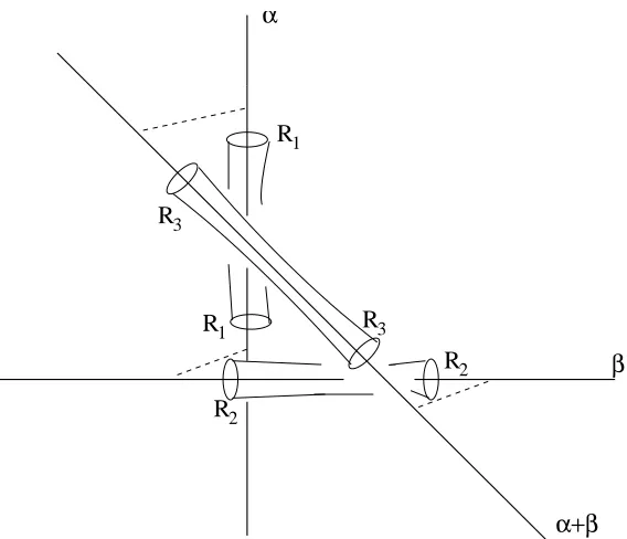
R2
R2 R1
R1 R3
R3
α
β
α+β
[image:23.612.167.451.420.664.2]The three-spheres in fig. 8 form a necklace where each is intersecting the other two over anS1, so we get scalar fields in the bifundamental, and integrating them out leaves us with the annuli shown in the figure. The path integral of the A-model in this background
involves four Chern-Simons theories on a chain of four three-spheres connected with annuli:
Z =
Z Y3 i=1
DAieSCS(Ai)O(U1, U2;r1)O(U2, U3;r2)O(U3, U1;r3) (4.7)
There are two unknots on each three-sphere, and the amplitude will depend on their linking, in addition to their framing. Just as above, we can use (4.5) to write this in a more transparent form
Z = X
R1,R2,R3
hR1|VM3R3ie
−ℓ3r3hR
3|VM2R2ie
−ℓ2r2hR
2|VM1R1ie
−ℓ1r1. (4.8)
Since the D-branes go around the loop from one degeneration locus to the other and then back to the first one, we must have
VM3VM2VM1 = 1.
This will hold generally whenever there are closed loops with D-branes in the toric diagram.
Fig. 9 The Hopf link with linking number lk = +1 .
Looking at fig. 8 we can read off,
VM1 =S
−1, V
M2 =ST
−1S, V
M3 =T S
−1, (4.9)
so that the last factor of (4.8) is given by
[image:24.612.229.375.445.534.2]This means that M1 is a three-sphere with two unknots that are linked into a Hopf link
L(R2, R1) of linking number lk = 1 (see fig. 9). Namely, as we have seen previously, S3 is obtained by identifying two solid tori up to an S transformation that exchanges the α
and the β cycles of theT2. Ifβ is the nontrivial cycle of the solidT2, and along this cycle one has a knot in representation R1 and another one in representation R2, then the S−1 transformation results in two unknots with zero framing (this does not add any twists to the ribbons that frame the knots), but which are linked in a Hopf link with linking number lk = 1 (an S transformation would give a Hopf link with linking number −1). Similarly, using ST−1S =T S−1T, we see that M
2 has a Hopf link with two knots of framing +1.
Z(M2,L(R3, R2)) =hR3|T S−1T|R2i. (4.11) Finally, M3 is a three-sphere with a Hopf link whose components are an unknot carrying representation R1 and with framing +1, and an unknot carrying representation R3 with canonical framing:
[image:25.612.181.432.394.632.2]Z(M3,L(R1, R3)) =hR1|T S−1|R3i. (4.12)
4.4. Lattice model interpretation
The models discussed above clearly generalize to more complicated geometries like the one depicted in fig. 10, where we have suppressed one direction of the base. The rules for computing the amplitudes should be clear from the previous discussion:
1) The model has states associated to all the edges of the lattice. Some of the edges are “primitive” (connecting nearest neighbor nodes) and some are “non-primitive” (connecting other nodes but always along the straight lines of the lattice) The states are labeled by representations of the affine Lie algebra (i.e. a state in the Hilbert space of T2, H). To each state on the i-th edge we associate a weight e−ℓri, where r
i is the length of the corresponding edge and the ℓ is the number of boxes in the corresponding representation.
2) To every vertex we associate a linear operator. This linear operator is obtained by computing matrix elements like the ones depicted below:
R2 4 R
~
R
3 R
1
R
< 1R |V| R R >2 3 4
Fig. 11The four-point vertex.
Here, R1, R2 and R3, R4 are the two pairs of representations corresponding to the collinear edges. A state |R, R′i is obtained by doing the Chern-Simons path integral over the solid torus with two parallel Wilson lines inserted along its nontrivial cycle, in representationsR,R′. V is the gluing matrix, as explained before. As is well known, using the fusion rules of the WZW theory, we can write
|R, R′i=X R′′
NRRR′′′|R′′i
where the fusion coefficients are given by the Verlinde formula [45]
NRRR′′′ =
X
Q
SRQSR′QS−1 R′′Q S0Q
, (4.13)
Using this we can write the four-point vertex as
hR1, R2|V|R3, R4i =
X
Q,Q′ NRQ
1R2VQQ ′NQ
′
whereV denotes the corresponding modular transformation matrix. Notice that, although there are four primitive edges ending on each vertex, one can have many non-primitive edges ending on the same vertex. In that case, we will have matrix elements of the form
hR1,· · ·, Rn|V|R′1,· · ·, R′mi (4.15) where the in- and out-states can be evaluated by a repeated use of the fusion rules. In (4.15), R1,· · ·, Rn correspond to a set of collinear edges, and R′1,· · ·, R′m to the other set. As explained before the solid tori are glued together by an SL(2,Z) matrix V that is computed as in (2.3).
3) Since there are edges that go off to infinity, there are boundary conditions: the state on these edges is always the trivial representation7.
4) The amplitude is the product of the linear operators over all the vertices, together with the weights associated to the connecting edges. At the end we sum over all represen-tations on each link.
5. Large N Duality
As was recently demonstrated [24], one can derive the large N duality conjecture of Chern-Simons on S3 with topological strings [1]. In this derivation one starts with the linear sigma model description of the closed string side and finds that in some limit the theory develops Coulomb and Higgs branch. The Coulomb branch plays the role of holes in the dual Chern-Simons description.
The models we are considering here all admit a linear sigma model description [46], as discussed in [47]. Thus one can start from the gravity side, and go to the point on moduli for eachU(1) gauge factor and repeat the analysis of [24], which should lead to topological open string description withNi D-branes wrapped around S3i. The analysis we did for the open string demonstrated that this open string can in turn be written in terms of some link observables in the product ofU(Ni) Chern-Simons theories. Thus we find the general prediction that
Fclosed(ti, ra′) =Fopen(Nigs, ra)
7 It would also be interesting to put periodic boundary conditions and interpret them as
where byFopen we mean the open string amplitude with link observables inserted, and the
ra correspond to sizes of the annuli. In this equation, the ti on the closed string side are the K¨ahler moduli of the blowups corresponding to where the S3i were, and ti =Nigs. As we will see later, r′a=ra− 12(ta1+ta2) where tai denote the K¨ahler moduli associated to the two ends of the annulus a. It would be interesting to repeat in detail the analysis of [24] for the case at hand and thus obtain these shifts directly.
6. Closed String Localization
In this section we argue that the largeN duality proposal given in the previous section is in accord with localization ideas in computation of the closed string invariants.
invariants where one uses Kontsevich’s results on matrix realization of Mumford classes [50] together with certain results of Faber [51]. However, the Chern-Simon gauge theory is a more natural realization of this computation.
7. Closed String Invariants from Chern-Simons Theory
In this section we will show that the largeN duality proposed in section 5 is a powerful way to compute closed string topological A-model amplitudes for local Calabi-Yau mani-folds, in terms of Chern-Simons amplitudes. In particular we will consider examples of IP2 blown up at three points (IB3 del Pezzo), and IP1×IP1 blown up at four points. Since the size of the blow ups are proportional to the rank of the corresponding dual gauge group, we can also consider the limit where the blown up IP1’s have infinite size by considering the Ni → ∞ limit. This in particular leads to computation of topological strings for IP2 and IP1×IP1 inside a Calabi-Yau threefold.
7.1. Chern-Simons Invariants of Unknots and Hopf Links
The toric geometries that we have described involve framed unknots and Hopf links, therefore in the evaluation of the Chern-Simons amplitudes we will need the invariants of the unknot and the Hopf link in arbitrary representations of SU(N). In this section we give precise formulae for these invariants. Our notation is as follows: WR1,R2(L) denotes
the vacuum expectation value in Chern-Simons theory corresponding to the link L with components K, K′:
WR1,R2(L) =hTrR1(U1)TrR2(U2)i, (7.1)
whereU1,U2are the holonomies of the gauge field around the knotsKandK′, respectively. If, sayR2 =·is the trivial representation, the vev (7.1) becomes the vev of the knotK(the second knot disappears), and we will denote this vev by WR(K). The vacuum expectation values denoted byh·iare normalized, so that they denote the path integral with insertions and divided by the partition function (in other words, the vev of the identity operator is one). Of course the duality also cares for the overall normalization (i.e., the vacuum energy) and this we will put in at the end of the computation. We also recall our notation for the Chern-Simons variables:
q = exp
2πi k+N
It is well-known that the Chern-Simons invariant of the unknot in an arbitrary repre-sentation R is given by the quantum dimension of R:
WR =
S0R
S00
= dimqR. (7.3)
The explicit expression for dimqR is as follows. Let R be a representation corresponding to a Young tableau with row lengths {µi}i=1,···,d(µ), with µ1 ≥ µ2 ≥ · · ·, and where d(µ) denotes the number of rows. Define the following q-numbers:
[x] =qx2 −q− x 2,
[x]λ =λ
1 2q
x 2 −λ−
1 2q−
x 2.
(7.4)
Then, the quantum dimension of Ris given by
dimqR=
Y
1≤i<j≤d(µ)
[µi−µj +j−i] [j−i]
dY(µ) i=1
Qµi−i
v=−i+1[v]λ
Qµi
v=1[v−i+d(µ)]
. (7.5)
The quantum dimension is a Laurent polynomial in λ±12 whose coefficients are rational
functions of q±12. In what follows in some cases we will also be interested in the leading
power ofλin the above expression. It is easy to see that this power isℓ/2, whereℓ=Piµi is the total number of boxes in the representation R, and the coefficient of this power is the rational function of q±12
qκR/4 Y
1≤i<j≤d(µ)
[µi−µj +j−i] [j−i]
dY(µ) i=1
µi
Y
v=1
1
[v−i+d(µ)], (7.6)
where
κR=ℓ+ d(µ)
X
i=1
µi(µi−2i). (7.7)
This quantity is related to the quadratic Casimir of the representation. In fact, one has ΛR·(ΛR+ρ) =κR+N ℓ−ℓ2/N.
Let us now consider the Hopf link with linking number 1. Its invariant for represen-tations R1, R2 is given by
WR1,R2 =q
ℓ1ℓ2/NS
−1 R1R2 S00
, (7.8)
where ℓi is the total number of boxes in the Young tableau of Ri, i = 1,2. The prefactor
the vev WR1,R2 has to be computed in the theory with gauge group U(N). Although the
expression for the S-matrix is explicitly known, it is not straightforward to write it in
terms of q and λ, which is what we need. We can use the Verlinde formula (4.13) giving
the fusion coefficients in terms of theS-matrix elements, as well as the well-known identity
(ST)3 =S2 =C, to obtain the expression
WR1,R2 =
X
R
NRR1,R2q12(κR−κR1−κR2)dim
qR. (7.9)
This can be also derived by using the formalism of knot operators [52][53], and it was
used in [5] to obtain the integral invariants associated to the Hopf link (we must observe,
however, that in [5] the Hopf link with linking number −1 was considered). Notice that
the fusion coefficients NR
R1,R2 become, in the large k limit, the Littlewood-Richardson
coefficients for the tensor productR1⊗R2 =PRNRR1R2R, and since we are evaluating the
invariants at largek, N, to compute (7.9) we have to use these tensor product coefficients.
Another expression for the Chern-Simons invariant of the Hopf link in arbitrary
repre-sentations has been recently obtained by Morton and Lukac by using skein theory [54][55].
Let us briefly describe their result, which turns out to be very useful in order to
com-pute the invariants. Let µ be a Young tableau, and let µ∨ denote its transposed tableau
(remember that this tableau is obtained from µ by exchanging rows and columns). The
Schur polynomial in the variables (x1,· · ·, xN) corresponding toµ (which is the character of the diagonalSU(N) matrix (x1,· · ·, xN) in the representation corresponding to µ), will be denoted by sµ. They can be written in terms of elementary symmetric polynomials
ei(x1,· · ·, xN), i≥1, as follows [56]:
sµ = detMµ (7.10)
where
Mµij = (eµ∨ i+j−i)
Mµ is an r×r matrix, with r = d(µ∨). To evaluate sµ we put e0 = 1, ek = 0 for k <0. The expression (7.10), known sometimes as the Jacobi-Trudy identity, can be formally
extended to give the Schur polynomial sµ(E(t)) associated to any formal power series
where ei denote now the coefficients of the series E(t), i.e. ei = ai. Morton and Lukac
define the series E∅(t) as follows:
E∅(t) = 1 + ∞
X
n=1
cntn, (7.11)
where the coefficients cn are defined by
cn = n
Y
i=1
1−λ−1 2qi−1
qi−1 . (7.12)
They also define a formal power series associated to a tableau µ, Eµ(t), as follows:
Eµ(t) =E∅(t) dY(µ) j=1
1 +qµj−jt
1 +q−jt . (7.13)
One can then consider the Schur function of the power series (7.13), sµ(Eµ′(t)), for any
pair of tableaux µ, µ′, by expanding Eµ′(t) and substituting its coefficients in the
Jacobi-Trudy formula (7.10). It turns out that this Schur function is essentially the invariant we
were looking for. More precisely, one has
WR1,R2 = (dimqR1)(λq) ℓ2
2 sµ
2(Eµ1(t)), (7.14)
where µ1,2 are the tableaux corresponding to R1,2, and ℓ2 is the number of boxes of µ2. More details and examples can be found in [54]. It is easy to see from (7.14) that the
leading power in λ of WR1,R2 is (ℓ1 +ℓ2)/2, and its coefficient is given by the leading
coefficient of the quantum dimension, (7.6), times a rational function of q±12 that can be
easily computed by taking λ → ∞in E∅(t).
As a simple example of the Morton-Lukac formula, we can compute W( , ). In this case, s{1} =e1, and it is enough to expand E{1}(t) at first order,
E{1}(t) = 1 +
n
1−q−1+ 1−λ −1
q−1
o
t+· · ·, (7.15)
so that we obtain
W( , )=
λ12 −λ− 1 2
q12 −q− 1 2
2
In the same way, one can easily find:
W( , ) =λ3
1−q2+q3 (q21 −q−
1
2)3(q+ 1)
−λ q
−1+ 1 +q3 (q12 −q−
1
2)3(q+ 1)
+λ−1 q
−1+ 1 +q2 (q12 −q−
1
2)3(q+ 1)
−λ−3 1
(q12 −q− 1
2)3(q+ 1) ,
W( , ) =λ3 q
−2−q−1+q (q21 −q−
1
2)3(q+ 1)
−λ q
−2+q+q2 (q12 −q−
1
2)3(q+ 1)
+λ−1 q
−1+q+q2 (q12 −q−
1
2)3(q+ 1)
−λ−3 q
(q12 −q− 1
2)3(q+ 1) ,
(7.17)
and so on. In the computations that give the invariants of IP2, we only need the rational function of q±12 which multiplies the highest power in λ.
The above results are for knots and links in the standard framing. The framing can be incorporated as in [8], by simply multiplying the Chern-Simons invariant of a link with components in the representations R1,· · ·, RL, by the factor
(−1)P
L
α=1pαℓαq 1 2
PL
α=1pακRα, (7.18)
where pα, α = 1,· · ·, L are integers labeling the choice of framing for each component.
7.2. Evaluation of the Two-Sphere Example 8
The simplest example of how to compute a closed string amplitude from Chern-Simons theory comes from the geometry depicted in fig. 6. As explained there, this involves computing the vacuum expectation value of the operator (4.5):
O(U1, U2;r) =
X
R
TrRU1e−ℓrTrRU2−1, (7.19)
where U1 and U2 are the holonomies of dynamical gauge fields (in other words, we are computing the vev in a U(N1)×U(N2) theory, but with the same coupling constant). We are going to discuss the operator (7.19) in a more general setting, so that U1 is the holonomy around an arbitrary knot. We are going to assume however that U2 is the holonomy around an unframed unknot. We now have to take the vev of this expression by doing the functional integral over both the U(N1) field A1 and the U(N2) field A2. Since
we are assuming that U2 is the holonomy around an unknot with zero framing, we have that [2]
hTrRU2−1iA2 = TrRU
−1
0 , (7.20)
whereU0 is the element in the Cartan subalgebra that corresponds to exp(2πiρ/(k2+N2)). Therefore, the vev with respect to the field A2 gives
hO(U1, U2;r)iA2 =
X
R
TrRU1e−ℓrTrRU0−1. (7.21) Notice that we can regard this vev as the generating functional considered in [2], where the source takes the particular value U0−1. We can now take the vev with respect to the
A1 field, and use the results of [2] to write:
hO(U1, U2;r)iA1,A2 = exp
X∞ d=1 1 d X R
fR(qd, λd1)e−dℓrTrRU0−d
, (7.22)
This expression is valid for any framed knot along which we take the holonomy U1 of the gauge field A1. In this equation, λ1 = qN1 is the exponential of the ’t Hooft coupling for the U(N1) Chern-Simons theory. We can write the exponent of the right hand side as follows,
X
R
fR(qd, λd1)e−ℓrTrRU0−d =
X
~k 1
z~k
f~k(qd, λd1)e−ℓrΥ~k(U0−d), (7.23) where f~k was introduced in [5] and is simply the character transform of the fR. The last factor can be easily computed to be
Υ~k(U0−d) =
Y j λ dj 2
2 −λ −dj
2
2
qdj2 −q− dj
2
kj
, (7.24)
where λ2 =qN2.
The vev (7.22) can be written in a very suggestive way by using the results of [5] on Chern-Simons vevs. In particular, f~k has the structure:
f~k(q, λ1) =
Y
j
(q−j2 −q j
2)kjX
g,Q
n~k,g,Q(q−
1 2 −q
1
2)2g−2λQ
1 . (7.25) Therefore, one finds for (7.22):
loghO(U1, U2;r)iA1,A2 =
∞ X d=1 X g,Q 1 d q −d 2 −q
d
22g−2X
~k
n~k,g,Q
z~k
e−dℓrY j
(λ− dj
2
2 −λ
dj 2
2 )kjλ dQ 1 ,
This has the structure of the free energy for a closed string [57]: ∞ X d=1 X g,m
ngm~ 1 d
2 sindgs 2
2g−2
e−d ~m·~t, (7.27)
provided one finds the appropriate relation between the closed string K¨ahler parameters~t, and the K¨ahler parameters for the open string appearing in (7.26). We will find the precise relation in the examples below. We also have to show that the expansion in (7.26) involves integers in a manifest way, since in (7.26) we are dividing the integers n~k,g,Q by z~k. The way to fix that is to recall that, as shown in [5], the “primitive” integer invariants are not
n~k,g,Q, but NbR,g,Q. They are related by a linear transformation involving the characters of the symmetric group,
n~k,g,Q =
X
R
χR(C(~k))NbR,g,Q. (7.28)
Using again the results of [5], one can show that
Y
j
(λ−j2 −λ j
2)kj = (λ−12 −λ 1
2)X
R
χR(C(~k))SR(λ−1), (7.29)
where SR(λ) is the monomial defined in [5]: if R is not a hook representation, it is zero, and if R is a hook of ℓ boxes with ℓ−s boxes in the first row, then
SR(λ) = (−1)sλ−
ℓ−1 2 +s
Using this, we find
X
~k
n~k,g,Q
z~k
Y
j (λ−
dj 2
2 −λ
dj 2
2 )kj = (λ −d
2
2 −λ
d 2
2)
X
R
SR(λ−d2 )NbR,g,Q, (7.30)
and this would lead to the identification
X
m
ngm~e−m·~ ~t = (λ− 1 2
2 −λ
1 2
2)
X
R,Q
e−ℓrSR(λ−21)λQ1NbR,g,Q
From this expression, together with a suitable linear map between K¨ahler parameters~tand (r, N1gs, N2gs) (which will lead to onlynegative exponents for~tand which will depend on the choice of knot), the integral structure on both sides is compatible and one can express the closed string integral invariants ngd in terms of the open string integral invariants
b
the relation will be rather simple. It is interesting to notice that, when N =M, i.e. both
gauge groups coincide, and r = 0, (7.19) is the partition function of the three-manifold
obtained after performing surgery on the knot where U is supported (for finite k and N)
[36][58][59].
The above result can be easily generalized to more complicated situations. For
exam-ple, one can consider L arbitrary knots,Kα, where α = 1,· · ·, L, and suppose that in each
of the components we have aU(Nα) Chern-Simons theory. Let us also considerL unknots
at zero framing Kα with a U(Mα) Chern-Simons theory in each of them. If we denote by
Uα, Vα the holonomies of the U(Nα), U(Mα) fields, respectively, one can construct the
operator
O(U1,· · ·, UL;V1,· · ·, VL) = exp
XL
α=1 ∞
X
n=1 e−nrα
n TrU
n
αTrVα−n
. (7.31)
Again it can be easily shown that logZ(U1,· · ·, UL;V1,· · ·, VL) has the structure of the free energy for a closed topological string.
As an application of the above computation, we can evaluate (4.6) when p = 0,
corresponding to fig. 6. In this case, U1 is the holonomy around an unknot with trivial framing, and the only nontrivial fR corresponds to the fundamental representation. We
then find,
Z(M1, M2) = exp(−F(M1)−F(M2)−F(M1, M2;r)) where F(Mi) is the free energy of the three-sphere Mi, and
F(M1, M2;r) = loghO(U1, U2;r)iA1,A2 =
∞
X
d=1
e−dr′(1−e−dt1)(1−e−dt2) d(2 sin(dgs/2))2
. (7.32)
Notice that, in writing (7.32), we have defined:
r′=r− t1+t2
2 , (7.33)
i.e. the parameter r that appears in (7.19) has to be renormalized in order to match the
closed string K¨ahler parameter r′. We will see below other examples of this, in which the
Fig. 12 After the transition, the two S3’s that we have wrapped D-branes on dis-appear, and with them all of H3(X), so we are left with b2(X) = 3.
The dual closed string geometry is depicted in fig. 12. The two S3’s, whose local neighborhood are T∗S3’s are replaced by two IP1’s with normal bundle O(−1)⊕ O(−1). In the total geometry, each of them intersects a IP1 with O ⊕ O(−2) normal bundle.
It is not difficult to calculate the genus zero amplitude of the closed string background using mirror symmetry, as in [25], and we find
Fg=0(r′, t1, t2) =
X
i=1,2 ∞
X
d=1 e−dti
d3 + ∞
X
d=1 e−dr′
(1−e−dt1)(1−e−dt2)
d3 ,
This has contribution from a single primitive curve in each of the classes [r′],[ti],[r+ti],[r+
t1 +t2]. In fact, the only primitive curves in this geometry are rational curves, which are enumerated by the genus zero amplitude. One easy way to see this is as follows.
Note that under the duality of M-theory on X/ type IIB theory on B×S1 that we discussed in the previous sections, M2 branes wrapping holomorphic curves in X that have components along theT2 directions map to (p, q) string web in type IIB string theory ending on the five-brane web (recall that M2 brane wrapping (p, q) cycle of theT2 maps to a (p, q) string in type IIB string theory). The requirement for supersymmetry is that the (p, q) string must be parallel to (p, q) five brane, and that stings must be parallel to the plane defined by the five-branes. Compact curves in X correspond to string webs ending on the five-branes, but not any string can end on any five brane – a (p, q) string can only end on the (p, q) five brane. These are conditions for holomorphic curves in X, rephrased in the IIB language (to be complete, there is also the zero force condition and string string charge conservation that must be conserved at each vertex, in addition to the junctions with five-branes).
This, together with the prediction for integrality properties of the amplitude (7.27), implies that the all genus partition function of the closed string theory is given by
F = ∞
X
d=1
e−dt1 +e−dt2 +e−dr′(1−e−dt1)(1−e−dt2) d(2 sin(dgs/2))2
(7.34)
This agrees exactly with the Chern-Simons answer (7.32). Note that
ti =Nigs
are two new K¨ahler parameters, the sizes of two-spheres that grow with N, replacing the
S3’s. The K¨ahler parameter r′ was already present in the open string geometry as the size of the holomorphic annulus with boundaries on the two spheres, but we have seen that their precise relation is given by (7.33).
7.3. O(−3)→IP2
The geometric transition in the three-sphere case is similar, and we have depicted it in fig. 3. The dual closed string geometry contains a IP2 with three exceptional IP1’s touching it at three points. We can send the size of these IP1’s to infinity by taking Ni → ∞in our calculation to recover the IP2 amplitude. The novelty in this case is that the closed string geometry has curves of arbitrarily high genus contributing to the topological A-model amplitudes, and infinitely many integer invariants are non-zero, as we will see.
K ’ K ’
K ’ K2 2 K3 3
K1 1
0
[image:38.612.121.489.471.560.2]0 1 1 0 1
Fig. 13The figure shows the Hopf links in the manifolds M1, M2 and M3
respec-tively. The numbers indicate the framing of each knot.
We now focus on the Chern-Simons computation that gives the invariants forO(−3)→
IP2. According to what we discussed before, the Chern-Simons scenario involves three different gauge groups, with ’t Hooft parameters t1, t2, t3, and with the same coupling constant gs. Accordingly, the quantum invariants will be a rational function of q and