Building Integral Projection Models: a User's Guide.

White Rose Research Online

[email protected]

Universities of Leeds, Sheffield and York

http://eprints.whiterose.ac.uk/

This is a copy of the final published version of a paper published via gold open access

in

Journal of Animal Ecology

.

This open access article is distributed under the terms of the Creative Commons

Attribution Licence (

http://creativecommons.org/licenses/by/3.0

), which permits

unrestricted use, distribution, and reproduction in any medium, provided the

original work is properly cited.

White Rose Research Online URL for this paper:

http://eprints.whiterose.ac.uk/78685

Published paper

‘HOW TO...’ PAPER

Building integral projection models: a user’s guide

Mark Rees

*, Dylan Z. Childs

and Stephen P. Ellner

1

Department of Animal and Plant Sciences, University of Sheffield, Western Bank Sheffield, S10 2TN, UK; and 2

Department of Ecology and Evolutionary Biology, Cornell University, Ithaca, NY 14853-2701, USA

Summary

1. In order to understand how changes in individual performance (growth, survival or repro-duction) influence population dynamics and evolution, ecologists are increasingly using parameterized mathematical models.

2. For continuously structured populations, where some continuous measure of individual state influences growth, survival or reproduction, integral projection models (IPMs) are commonly used.

3. We provide a detailed description of the steps involved in constructing an IPM, explaining how to: (i) translate your study system into an IPM; (ii) implement your IPM; and (iii) diag-nose potential problems with your IPM. We emphasize how the study organism’s life cycle, and the timing of censuses, together determine the structure of the IPM kernel and important aspects of the statistical analysis used to parameterize an IPM using data on marked individuals.

4. An IPM based on population studies of Soay sheep is used to illustrate the complete process of constructing, implementing and evaluating an IPM fitted to sample data.

5. We then look at very general approaches to parameterizing an IPM, using a wide range of statistical techniques (e.g. maximum likelihood methods, generalized additive models, non-parametric kernel density estimators). Methods for selecting models for parameterizing IPMs are briefly discussed.

6. We conclude with key recommendations and a brief overview of applications that extend the basic model. The online Supporting Information provides commented R code for all our analyses.

Key-words: integral projection model, mathematical model, Soay Sheep, structured population

Introduction

The development of data-driven, study-specific models is now commonplace in population biology (Ozgul et al. 2010; Brunoet al. 2011; Childset al. 2011; Wallace, Les-lie & Coulson 2013). These models are often used to explore the implications of environmental or experimental changes in individual-level demography at the population level, for example how do size-specific harvesting rates influence population dynamics and trait evolution (Wal-lace, Leslie & Coulson 2013). The most commonly used data-driven models are matrix projection models (MPM), which project discrete population structure (e.g. age or size class) in discrete time. These models are well under-stood mathematically and there is a well-developed

toolbox of techniques for their analysis (Caswell 2001). A major constraint on these models for populations where individuals are characterized by continuous variation is the assumption that individuals can be classified by a small number of discrete states, say for a size-structured population, small, medium and large individuals.

In some animal populations, an individual’s fate is often well predicted by their age or life stage (e.g. mature vs. immature), and matrix projection models yield a good description of population-level processes. However, in many populations, a continuous trait such as body mass is a key determinant of performance: all else being equal, larger individuals tend to exhibit greater survival and fecundity, so using a continuous state variable will be more appropriate and often improve the performance of the model (Ramula, Rees & Buckley 2009). In other cases, the whole purpose of developing a model is to understand

*Correspondence author. E-mail: [email protected]

how a continuous trait impacts ecological and evolution-ary processes (Coulson, Tuljapurkar & Childs 2010; Coul-son 2012). For example, Ozgulet al.(2010) explored how changes in body mass associated with environmental change mediated an historic shift in the population dynamics of a yellow-bellied marmot (Marmota flaviven-tris) population. In such settings, a framework for work-ing with continuous trait variation is needed.

Easterling, Ellner & Dixon (2000) originally proposed the integral projection model (IPM) as an alternative to matrix projection models for populations in which demo-graphic rates are primarily influenced by a continuously varying measure of individual size or state. Their model was deterministic and density-independent, analogous to a matrix projection model with a constant matrix (Caswell 2001). Since then, IPMs have developed considerably and now there are a wide range of methods available for anal-ysing populations with complex life cycles, time lags, den-sity dependence, environmental stochasticity and where individuals are distributed in space (Childs, et al. 2003, 2004; Ellner, & Rees 2006, 2007; Kusset al.2008; Rees & Ellner 2009; Coulson, Tuljapurkar & Childs 2010; Jonge-jans et al.2011; Ellner & Schreiber 2012). An R package for parameterizing and analysing some types of IPM is also now available (Metcalfet al.2013).

These mathematically sophisticated papers assume that an IPM has been constructed and parameterized, and pro-vide methods for analysing the resulting model. However, in the development of IPMs, relatively little has been writ-ten about: (i) the basic construction of an IPM, and in particular about how different life cycles and census times determine the structure of an IPM and (ii) appropriate statistical analyses for model parametrization, in particu-lar model diagnostics and alternatives to simple paramet-ric models. In this paper, we provide a detailed description of the entire process from data to implementa-tion of the IPM. Specifically we: (i) briefly describe the mathematical background to IPMs for those unfamiliar with the approach; (ii) provide a careful description of how to map your study system onto an IPM, dealing with how the life cycle and census times determine the struc-ture of the IPM and the statistical analysis; and (iii) look at model diagnostics, for the IPM structure, fitted func-tions and implementation. Finally, we present methods for relaxing some of the common statistical assumptions used for constructing IPMs; we look at more general regression models, and the use of GAM and kernel esti-mators which allow very flexible descriptions of the mean and distribution of residuals about the fitted demographic models, respectively.

To illustrate the process of building an IPM, we gener-ate artificial data using an individual-based model of the Soay sheep (Ovis aries) population on St. Kilda (Clutton-Brock & Pemberton 2004). Throughput the paper, we provide R code for each step, so readers can easily imple-ment an IPM for their study system.

We assume ‘ideal’ data: individuals are reliably marked, accurately measured and can be refound at each census if still alive, and otherwise presumed dead. Many plant studies achieve this ideal, and some animal studies (such as the Soays) come close. Reviewing the specialized tools for imperfect recapture, open populations and similar issues (e.g. www.phidot.org/software/mark) would greatly lengthen the paper, and capture–recapture analysis with continuous covariates is still under development (Langrock & King 2013), so it would be premature to offer advice. We also limit ourselves to model construc-tion and implementaconstruc-tion, and say nothing about estimat-ing the uncertainty in estimates or projections. About that, however, we can offer advice: bootstrap. The meth-ods for data resampling, standard errors, etc. in matrix population models (e.g. Kalisz & McPeek 1992; McPeek & Kalisz 1993; Caswell 2001, Ch. 12) are all directly applicable to IPMs.

Key assumptions and model structure

Individuals within a population typically vary in many different ways, but for simplicity, we assume that varia-tion among individuals is completely summarized by a single quantity z, which describes an individual’s state (e.g. size, fat stores), and this determines its fate. We often refer to z as ‘size’, meaning some continuous mea-sure of body size such as total mass or the log of snout-to-vent length. However, z can be unrelated to size – for example, it could be the individual’s spatial location in a linear habitat such as a riverbank, or a bird’s first egg-laying date. However, z must have finite limits: a minimum possible value L and a maximum value U. Ideally, z will be the character or set of char-acters most strongly linked to individual survival, growth and reproduction, though zcannot be, for exam-ple, an individual’s realized growth rate or fecundity. The premise of an IPM is that individuals with the same current state z have the same odds of different future fates and states, but what actually happens involves an element of chance.

The state of the population at timetis described by the size distributionn(z,t). Technically, for each timet,n(z,t) is a smooth function ofzsuch that

The number of individuals with trait valuezin the interval

[a;bat timetis¼ Z b

a

nðz;tÞdz: eqn 1

bell-shaped curve that characterizes the relative frequency of different possible values in a Gaussian distribution, and its integral from L to U is the total number of individuals.

Between times t and t+1, individuals can grow, shrink or die, and they can produce offspring that vary in size. To describe the net result of these processes, we define two functions P(z′,z), representing survival and growth or shrinkage, and F(z′,z) representing the production of new recruits. In both of these,zis size at timet andz′is size at time t+1. For an individual of size z at time t, P(z′,z)h is the probability that the individual is alive at time t+1, and its size is in the interval [z′,z′+h] (as with n(z,t) this is an approximation that is valid for small h, and the exact probability is given by an integral like eqn 1). Similarly, F(z′,z)h is the number of new offspring in the interval [z′,z′+h] present at time t+1, per size-z individual at timet.

It is often convenient to breakPup into two processes: size-dependent survival and size transitions fromz?z′, for example

Pðz0;zÞ ¼sðzÞGðz0;zÞ eqn 2

wheres(z) is the survival probability, andG(z′,z) describes size transitions. Note that G(z′,z) is not the probability density for the joint distribution of initial and subsequent sizes; rather, it is a family of univariate probability densi-ties for subsequent sizez′that depends on initial sizez. If you are not familiar with probability densities and how they differ from probabilities, see Appendix 1. Examples ofF(z′,z) will be presented in following sections.

The net result of survival and reproduction is summa-rized by the function

Kðz0;zÞ ¼Pðz0;zÞ þFðz0;zÞ eqn 3

called the kernel – we will refer to P(z′,z) and F(z′,z) as the survival and reproduction components of the kernel, or as the survival and reproduction kernels. The popula-tion at timet+1 is just the sum of the contributions from each individual alive at timet,

nðz0;tþ1Þ ¼

Z U

L

Kðz0;zÞnðz;tÞdz: eqn 4

The kernel Kplays the role of the projection matrix in a matrix projection model (MPM), and eqn (4) is the analogue for the matrix multiplication that projects the population forward in time.

P andF have to be smooth functions for these defini-tions to make sense. We have previously assumed that they are continuous (Ellner & Rees 2006), but it is actually sufficient forPandFto be piecewise continuous. This means that an IPM can include piecewise regression models, such as fecundity that jumps from zero to a positive value once individuals reach a critical ‘size at maturity’.

From life cycle to model: specifying a simple IPM

The kernelsPandFdescribe all the possible state transi-tions in the population, and all possible births of new

s(z)

p

r

n(z,t) _n(z′,t+1)

n(z,t)

s(z)

G(z_′,z)

G(z_′,z)

n(z_′,t+1)

pb(z)b(z) C₁(z′,z)

pb(z)b(z)C₀(z′,z) (a)

(b)

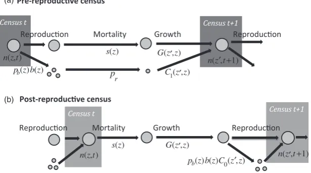
Fig. 1. Life cycle diagram and census points for (a) pre-reproductive and (b) post-reproductive census. The sequence of events in the life cycle is the same in both cases. However, the diagrams are different because reproduction splits the population into two groups [those who were present at the last census (large circles), and new recruits who were not present at the last census (small circles)], while at a census time the two groups merge. Reproduction is described by a two-stage process withpb(z) being the probability of reproduction

andb(z) being the size-specific fecundity. Each new recruit has a probabilityprof successful recruitment, and its size at the next census

is given byC1(z′,z). The pre-reproductive census leads to IPM kernelK(z′,z)=s(z)G(z′,z)+pb(z)b(z)prC1(z′,z) whereC1(z′,z) is the size

dis-tribution of new recruits at age 1 (when they are first censused). The post-reproductive census leads to IPM kernelK(z′,z)=s(z)G(z′,z)+

s(z)pb(z)b(z)C0(z′,z) whereC0(z′,z) is the size distribution of new recruits at age 0 (when they are first censused). The termpris absent in

recruits. But where do these kernels come from? In this section, we answer that question by showing how to trans-late population census data into a simple deterministic IPM for a size-structured population. We will describe how information on growth, survival and reproduction is combined to make a kernel. As IPMs are data-driven, our aim is to show how to arrive at a model which is both consistent and feasible. By consistent, we mean a model that accurately reflects the life cycle and census regime. By feasible, we mean a model that can also be parameterized from the available data. In the case study below, we will then take the next step of fitting specific models to data.

The key idea is that the kernel is built up from func-tions that describe a step in the life cycle of the species, based on the data about each step. Throughout, we assume that the data were obtained by marking individu-als, and following them over their life cycle with evenly spaced censuses at timest =0,1,2,⋯.

We strongly recommend that you begin by drawing a life cycle diagram indicating when demographic processes and census points occur, see Fig. 1. For this first exam-ple (Fig. 1a), we assume that at each time step, there is a single census point immediately prior to the next occur-rence of reproduction (i.e. there is a pre-reproductive cen-sus). At that time, you record the size of each individual. At time t+1, the population will include survivors from time t and new recruits. We assume, for now, that you can assign offspring to parents and therefore can record how many offspring each individual has giving you a data table like this:

Sizet Offspring

3 0

7 5

8 4

Combining this with the size measurements taken at time t+1, we end up with a table suitable for statistical analysis:

Sizet Offspring Survive Reproduced Sizet+1

3 0 0 0 NA

7 5 1 1 8

8 4 1 1 10

where we have added two indicator variables for survival (did the individual survive to t+1?) and reproduction (did the individual have any new offspring?).

To define the structure of the IPM, we can begin by ignoring individual size and constructing a model for the dynamics of N(t), the total number of individuals at cen-sus t that reflects the life cycle and data. Each individual at time t can contribute to N(t+1) in two ways: survival and reproduction.

1 Survival: Having observed how many individuals sur-vive from each census to the next, you can estimate an

annual survival probabilitys. At timet+1, the popula-tion then includessN(t) survivors from timet.

2 Reproduction: We could similarly define a per-capita fecundity b, and let prbN(t) be the number successful recruits at time t+1, with pr being the probability of successful recruitment. But the data distinguish between ‘breeders’ and ‘non-breeders’, so we can be more mechanistic. Let pb denote the probability that an individual reproduces, and b the mean clutch size among individuals that reproduce. Then, the number of new recruits at timet+1 ispbprbN(t).

Combining survivors and recruits, we have the unstruc-tured model

Nðtþ1Þ ¼sNðtÞ þpbprbNðtÞ ¼ ðsþpbprbÞNðtÞ: eqn 5

The ‘kernel’ for this model isK=s+pbprb, which is just a single number because at this point, the model ignores the size structure of the population.

The next step is to incorporate how the size at time t affects these rates: the probability of surviving, the probability of reproducing and the number of offspring are all potentially functions of the individual’s current sizez:

s¼sðzÞ; pb¼pbðzÞ; b¼bðzÞ:

Our prediction ofN(t) can now take account of the cur-rent size distribution,n(z,t),

Nðtþ1Þ ¼

Z U

L

sðzÞ þpbðzÞprbðzÞ

ð Þnðz;tÞdz: eqn 6

At this next level of detail, the kernel is a function of cur-rent sizez,K(z)=s(z)+pb(z)prb(z).

What is missing from model (6) is the size distribution at time t+1. To forecast that, we need to specify the size distributions of survivors and recruits. These are given by the growth kernel for survivors, G(z′,z), and the size dis-tribution of recruits, C1(z′,z), as described in Section Key assumptions and model structure, giving us the complete kernel

Kðz0;zÞ ¼sðzÞGðz0;zÞ þpbðzÞprbðzÞC1ðz0;zÞ: eqn 7

for the general IPM (eqn 4). So the structure of the kernel is determined by the life cycle and when the population is censused.

Size(t) Offspring Survive Reproduced Size(t+1)

3 NA 0 NA NA

7 5 1 1 8

8 4 1 1 10

The main difference to notice here is that for individu-als that die before the next census, there are now NA’s in the Offspring and Reproduced column. This has to be so, because the life cycle in this case has mortality occurring beforereproduction. As a result, the structure of kernel in this case is

Kðz0;zÞ ¼sðzÞGðz0;zÞ þsðzÞpbðzÞbðzÞC0ðz0;zÞ: eqn 8

In order to reproduce individuals now have to survive, hences(z) is a factor in both the survival and reproduction components of the kernel. The absence of theprterm is a consequence of censusing the population immediately after reproduction. Newly produced individuals do suffer mortal-ity before their next census at age 1, but this is included in thes(z) term because already at age 0 they are part ofn(z,t) (Fig. 1b). The functionspb(z) andb(z) are now the probabil-ity of reproducing, and mean number of offspring produced, for individuals that survive the time step. The NA’s in the data table will make sure that you ‘remember’ this, and only data on survivors to fit these functions.

When reproduction occurs just before the next census (as in Fig. 1b), pb andb could be fitted instead as func-tions of z′, the size at the post-breeding census which is also the size when reproduction occurs. This seems more natural, but it leads to a more complicated model. In that approach, the steps to producing size-z′offspring are: sur-vive and grow to some size z*, breed or not (depending onz*) and if so have b(z*) offspring, some of which are sizez′. The fecundity kernel needs to total this up over all possible sizesz*, which is:

Fðz0;zÞ ¼sðzÞ

ZU

L

Gðz*;zÞpbðz*Þbðz*ÞC0ðz0;z*Þdz*: eqn 9

Alternatively, the interval between censuses can be broken up into survival/growth (t to t+s) and reproduction (t+s tot+1) phases with separate kernels:

nðz*;tþsÞ ¼

ZU

L

sðzÞGðz*;zÞnðz;tÞdz

nðz0;tþ1Þ ¼nðz*;tþsÞ

þ ZU

L

pbðz*Þbðz*ÞC0ðz0;z*Þnðz*;tþsÞdz*

eqn 10

We think that eqn (8) is simpler. When you fitpbandb as functions ofz, you are in effect letting the data do the

integrals with respect to z* for you, because the fitted models will represent the average breeding probability and fecundity with respect to the distribution of possible sizes when reproduction occurs.

The size distribution of new recruits will also vary depending on the timing of the census. In the post-repro-ductive census, C0(z′,z) is the size distribution of recruits at age 0 immediately after their birth (or so we assume). In the pre-reproductive census, recruits were born imme-diately after the previous census, so they have already undergone a period of growth before they are first observed, and so C1(z′,z) is the distribution of new recruits aged 1.

In contrast to the fecundity kernel, the survival kernels in (7) and (8) are the same. Indeed, so long as the demo-graphic models are all based on z (initial size), it does not matter where growth falls in the sequence of events, or if growth is instead a continuous process that overlaps with mortality and reproduction. If you know each indi-vidual’s initial size and whether or not it survived through the next year, those are the data to whichs(z) is fitted. If you know the final size of all survivors, those (initial size, final size) pairs are the data to which G(z′,z) is fitted.

If there are multiple censuses per year, the additional measurements can inform the construction of the kernel, in particular the order of events in the life cycle diagram can reflect the additional information. Multiple censuses also mean that we have to decide when we are going to project the population’s state. This will typically be one of the census times but might not, say if we used average or maximum size over several censuses as our measure of size. Alternatively, the annual projection could be broken up in to several census-to-census projections as in eqn (10), like a seasonal matrix projection model. In Appendix 4, we use the Soay sheep case study to present one approach to constructing an IPM when there are several censuses within an annual cycle. In some systems, there may be additional time delays, say because reproduction is better predicted by an individual’s state at timet1. This leads to a time-lagged IPM, where the state of the popula-tion at timet+1 depends the survival and growth of indi-viduals at timet and the recruitment of new individuals, which depends on the size structure at time t1 (Kuss et al.2008).

The life cycles considered in this section are just two of the simplest possibilities, and many organisms could not be shoehorned comfortably into either of them. In Appen-dix 4, we use the Soay sheep system to present a general approach for situations where the sequence of events is more complicated and different data are taken at various times in the year. The important message of this section is that the structure of the IPM is jointly determined by the timing of the census and the order of events in the life cycle, and both these also have important consequences for the statistical analyses to estimate the demographic functions making up the kernel.

Numerical implementation

The one-variable IPM (4) is easy to implement numerically with a numerical integration method called midpoint rule (Ellner & Rees 2006). Definemesh points ziby dividing the size range [L,U] into m artificial size classes of width h=(UL)/m, and letzibe the mid-point of theith size class:

zi¼Lþ ði05Þh; i¼1;2;. . .;m: eqn 11

The mid-point rule approximation to eqn (4) is then

nðzj;tþ1Þ ¼h

Xm

i¼1

Kðzj;ziÞnðzi;tÞ: eqn 12

In R (see Box 1), we arrange the hK(zj,zi) terms in a matrix called theiteration matrix. This allows us to iterate the model by matrix multiplication and use the wide range of numerical tools available for matrices.

The only drawback to mid-point rule is that it is not very efficient relative to higher-order integration methods, so sometimes it takes a very large iteration matrix to get accurate results. In the section ‘Model diagnostics’ we give some pointers on choosing the size of the iteration matrix and the size limits L,U, and mention some alter-natives to mid-point rule.

Case study

So far we have looked at translating your study system into an IPM and how to solve the model numerically. In this section, we will put all this together, to show you that building a basic IPM is really pretty straightforward: there is no black magic or black boxes. To do this, we will develop a case study for an idealized animal system, based on published empirical studies. We will simulate data from an individual-based model (IBM) – a simula-tion that tracks individuals – and analyse the resulting data to build an IPM.

Our example explores the body mass-structured dynamics of an ungulate population: the feral Soay sheep (O. aries) of the island of Hirta in the St. Kilda archipelago, off the north-west coast of Scotland. We

have chosen to base our example on this population because it has been a major target of research into the dynamics and evolution of wild populations (Clutton-Brock & Pemberton 2004). Although we use simulated data, the IBM was parameterized using the Soay sheep data set. The advantage of using simulated data is that we know the underlying process that generated the data and so can see how various modelling assumptions influ-ence our results. Our aim is to outline a general approach for moving from an individually structured data set to a fully parameterized IPM. The resulting workflow can be applied to almost any life history that can be approximated as a sequence of transitions in dis-crete time.

s u m m a r y o f t h e d e m o g r a p h y

We assume that our simulated population is similar to the real Soay sheep population, but with a few impor-tant simplifications. The St. Kilda population has been studied in detail since 1985. Each year during this

Box 1. Implementing mid-point rule in R

# your code, for example

# return(s(z)* G(z1,z))

# using functions s and g that you have defined

}

F_z1z<- function(z1,z,m.pars){

# your code

}

Herem.parsis a vector of model parameters. The next step is to compute the mesh points:

L<- 1; U<- 10 # size range for the model

m<- 100 # m is the size of the iteration matrix

h<- (U-L)/m

meshpts<- L+(1:m)*h - h/2

The R functionoutermakes it easy to compute the iteration matrix:

P<- h * (outer(meshpts, meshpts, P_z1z))

F<- h * (outer(meshpts, meshpts, F_z1z))

K<- P+F

We put this code inside a functionmk_Kwhich has four arguments: the number of mesh points, the parameter vector and the two integration limits, so mk K (nBigMatrix, m.par.true, min.size,

max.size)

returnsP,F,Kcalculated using the parameters in m.par.trueusingnBigMatrixmesh points from size

period, newborn individuals are caught, weighed and tagged shortly after birth in the spring, and body mass measurements are taken from approximately half the population each summer during the August catch. Maternity is inferred from detailed field observations and genetic data, while periodic censuses and mortality searches ensure that individual mortality status and pop-ulation density are very well characterized. Since body mass data on established individuals and new recruits are only available during the August catch, it makes sense to choose this date as our census point to project the dynamics from. Almost all of the mortality in the system occurs during the winter months when forage availability is low and climate conditions are harsh (Clut-ton-Brock & Pemberton 2004).

These features of the life history and census regime mean that the life cycle diagram for the Soay system cor-responds to the post-reproductive census case in Fig. 1b, that is, survival precedes reproduction and individuals are censused prior to the key mortality period. A potential problem with assuming this sequence of events is that only adults that survive from one August catch until the next contribute new recruits to the population, despite the fact that lambing occurs several months earlier in the spring. This is demographically equivalent to assuming that any reproducing individual that dies between giving birth in the spring and the August catch will fail to raise viable offspring. With a handful of exceptions, this is pre-cisely what is observed in the Soay system, so we consider this to be a reasonable assumption.

To keep our example tractable, we will make a number of simplifications: (i) we only consider the dynamics of females; (ii) we ignore the impact of age structure; (iii) we assume that the environment does not vary among years, either as a result of density dependence (e.g. resource limi-tation) or abiotic factors (e.g. winter weather); and (iv) we assume that Soay females only bear singletons, though in reality they produce twins at a rate 10–15% in any given year. All of these assumptions can be relaxed, although the resulting model is rather more complicated (Childs et al.2011). We work with natural log body mass, based on the analysis of the real data; in Appendix 2, we discuss why log-transformed size is often a good choice for IPMs. The individual-based model is described fully in Appendix 3, and the R code is inUngulate Simulate IBM.R in the Supporting information.

d e m o g r a p h i c a n a l y s i s

The results of the IBM simulation are stored in an R data frame (calledsim.data), with columns z, z1 containing the sizes in yeartandt+1; indicator variables for survival (Surv = 1 if survived), reproduction (Repr = 1 if repro-duced) and recruitment (Recr=1 if recruited); and a final column for recruit size (Rcsz). We should check the data set carefully to make sure it has the structure we are expecting.

z Surv z1 Repr Recr Rcsz

3.07 0 NA NA NA NA

3.17 1 3.24 1 1 2.47

3.02 1 3.17 0 NA NA

2.92 0 NA NA NA NA

3.14 1 3.25 0 NA NA

3.06 1 3.00 0 NA NA

Inspection suggests this data set is as we expect. For example, individuals that die (Surv=0) have missing val-ues (NAs) in all the other columns, and the individuals that survive (Surv=1) but fail to reproduce (Repr=0) have a sequence of missing values for the three remaining vari-ables describing offspring recruitment.

Since we know how the data were generated, we can fit the ’right’ models to the data; we will deal with methods for model criticism later. Survival is modelled by a logistic regression, so we fit it by

mod.Surv<

-glm(Surv∼z , family=binomial, data=sim.data) The same is true for whether or not a female repro-duced (Repr), and whether or not that lamb survived to recruit into the population their first summer (Recr), mod.Repr<

-glm(Repr∼z, family=binomial, data=sim.data)

mod.Recr<

-glm(Recr∼1, family=binomial, data=sim.data) Note that mod.Recr does not have any dependence on mother’s size z, so it is estimating a single number: the recruitment probability. The subsequent sizes of new recruits and of surviving adults are fitted by linear regression,

mod.Grow<- lm(z1∼z, data=sim.data)

mod.Rcsz<- lm(Rcsz∼z, data=sim.data)

All the models were fitted using the sim.data data frame, which was possible as the NAs ensure that only appropriate individuals are included in each analysis.

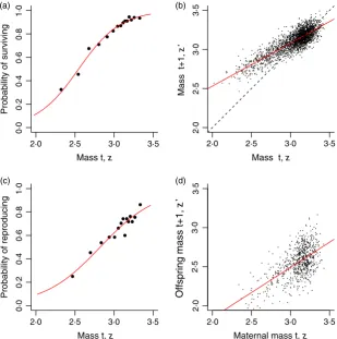
The fitted models are summarized in Fig. 2, and all of the models look reasonable as expected. Having fitted the various models, we then store the parameter estimates in m.par.est, using the same order and names as the parameter vector from the IBM (m.par.true).

m.par.est<- c(

## survival

surv=coef(mod.surv.glm),

## growth

grow=coef(mod.grow),

grow.sd=summary(mod.grow)$sigma,

## reproduce or not

repr=coef(mod.repr),

## recruit or not

recr=coef(mod.recr),

## recruit size

rcsz=coef(mod.rcsz),

rcsz.sd=summary(mod.rcsz)$sigma)

i m p l e m e n t i n g t h e i p m

The next step is to write down the kernel and check whether its formulation matches our knowledge of the life cycle and the data collection protocols,

Kðz0;zÞ ¼sðzÞGðz0;zÞ þsðzÞpbðzÞprC0ðz0;zÞ=2: eqn 12

In this instance, both the survival and reproduction kernel components contain the s(z) term, because the main period of mortality occurs prior to reproduction. The survival component includes the growth kernel G(z′, z); as in the example below, Gis often specified in terms of the conditional mean, variance and distribution fam-ily of subsequent size. The reproduction component is simply the product of the reproduction function, pb(z), the probability of survival from spring until summer, pr, and the conditional offspring size function, C0(z′,z). The factor of 1/2 appears because we are tracking the dynamics of females and have assumed an equal sex ratio.

We are going to use the approach given in Box 1, so we need to specify theP(z′,z) andF(z′,z) functions: ## Define the survival-growth kernel

P z1z<- function (z1, z, m.par){

return(s z(z, m.par) * G_z1z(z1, z, m.par)) }

## Define the reproduction kernel

F z1z<- function (z1, z, m.par){

return( s z(z, m.par) * pb_z(z, m.par) * (1/2) *

pr_z(m.par) * C_0z1(z1, z, m.par) ) }

These are just R translations of the two kernel compo-nents, and each function is passed a numeric vector, m.par, that holds the parameter values for the underlying demographic regressions. In order to complete the imple-mentation of our model, we next need to define the vari-ous functions called within P_z1z and F_z1z. These follow in a very intuitive way from the statistical models we fitted to data. For example, the function describing the probability of survival is:

s z<- function(z, m.par){

linear.p<- m.par["surv.int"]+m.par["surv.z"] * z

# linear predictor

p<- 1/(1+exp(-linear.p))

# inv-logistic trans

return(p) }

pb z<- function(z, m.par){

linear.p<- m.par["repr.int"]+m.par["repr.z"] * z

p<- 1/(1+exp(-linear.p))

return(p)

}

These functions extract the appropriate parameters, calculate the linear predictor at each value ofz and then transform this onto the probability scale. For s_z and Mass t, z

Probability of surviving

Mass t, z

Mass t+1,

z

’

Mass t, z

Probability of reproducing

2·0 2·5 3·0 3·5 2·0 2·5 3·0 3·5

2·0 2·5 3·0 3·5

2·0 2·5 3·0 3·5

0·0

0·2

0·4

0·6

0·8

1·0

0

·00

·2

0

·40

·6

0

·81

·0

2·0

2·5

3

·0

3·5

2·0

2·5

3·0

3·5

Maternal mass t, z

Offspring mass t+1,

z

’

(a) (b)

(c) (d)

Fig. 2. The main mass-dependent demo-graphic processes in the Soay sheep life cycle, as a function of current size,zin year

t. (a) The probability of survival, (b) female mass in the next summer census (August catch), (c) the probability of reproduc-tion and (d) offspring mass. Source file:

pb_z, the output is a number, the probability of the event in question, butG(z′,z) needs to evaluate a function, the probability density function for size at the next census. To do this, we use the regression ofz′onzto calculate a sheep’s expected size at the next census given its current size. The standard deviation of z′ is determined by the scatter about the regression line in Fig. 2b, which we also estimate from the fitted regression. Finally, because the deviations about the fitted line are assumed to follow a Gaussian distribution, we calculate the probability density of observing a sheep of sizez′ given its current size using dnorm.

G z1z<- function(z1, z, m.par){

mu<- m.par["grow.int"]+m.par["grow.z"] * z

# mean size next year (z1)

sig<- m.par["grow.sd"]

# sd about mean

p.den.grow<- dnorm(z1, mean=mu, sd=sig)

# pdf for size z1

return(p.den.grow) }

Finally, we calculate the probability density function for recruit size at the next census, given parental size in the current census, which uses the same approach. C 0z1z<- function(z1, z, m.par){

mu<- m.par["rcsz.int"]+m.par["rcsz.z"] * z

# mean size of recruits next year

sig<- m.par["rcsz.sd"]

# sd about mean

p.den.rcsz<- dnorm(z1, mean=mu, sd=sig)

# pdf for offspring size z1

return(p.den.rcsz) }

The final step in implementation is choosing the size range and number of mesh points. Because large individ-uals tend to shrink and their offspring are much smaller than themselves (Fig. 2b,d), the upper limit just needs to be slightly larger than the largest observed size, and we setU =355. The smallest individuals tend to grow, but they have a small chance of breeding and having off-spring who are even smaller than themselves. To make sure that the IPM includes those individuals, we can compute the mean offspring size for the smallest observed size (z2) and subtract off two standard devia-tions of offspring size:

m.par.est["rcsz.int"]+m.par.est["rcsz.z"]*2

2* m.par.est["rcsz.sd"]

1.523043

So we take L=15. The total size range is UL 2 units on log scale. We will use 100 mesh points so that the increment between mesh points is 002 units on log scale, which is about a 2% difference in body mass, see Section Model diagnostics.

b a s i c a n a l y s i s

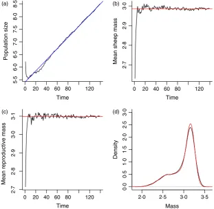
There is no density dependence in the Soay IBM, so we expect the population to grow or shrink exponentially and this is indeed what we find, Fig. 3a. The finite growth rate of the population (k) estimated from the simulation

Time

Population size

Time

Mean sheep mass

Time

Mean reproductive mass

5·5

6·0

6·5

7·0

7·5

8·0

8·5

2·7

2·8

2·9

3·0

0 20 40 60 80 120

0 20 40 60 80 120 0 20 40 60 80 120

2·7

2

·8

2·9

3

·0

3·1

2·0 2·5 3·0 3·5

0·0

0

·5

1·0

1

·5

2·0

2

·5

3·0

Mass

Density

(a) (b)

(c) (d)

by regressing log population size against time is ∼ 1022, so the population is growing by about 2% each year in the IBM. We can estimate the growth rate using the IPM as follows: (i) use the mk_K function with the estimated model parameters m.par.est to make an iteration matrix; (ii) use the eigen function to compute the domi-nant eigenvalue of this matrix, which is our estimate of the population growth rate (Easterling, Ellner & Dixon 2000). When we do this, we find that the fitted IPM pre-dicts akof 1022, the observed population growth rate in the IBM. Ellner & Rees (2006) review stable population growth theory, which covers the existence of a unique sta-ble population distribution and asymptotic growth rate, which a density-independent population converges to from any initial composition.

The fitted IPM can be used to calculate a wide range of statistical summaries of the population (Rees & Rose 2002). For example, in the IBM, both the mean size and mean reproductive size appear to approach a stable value, Fig. 3b,c. Both these expectations are straightforward to calculate from the stable size distribution,w(z), which can be calculated using theeigenfunction. This is just a mat-ter of extracting the dominant eigenvector w of the itera-tion matrix and normalizing it to a discrete probability density function, stable.z.dist.est<- w/sum(w). The vectorstable.z.dist.estcan be thought of as the fre-quency distribution for a set of narrow size classes centred at the values in themeshptsvector defined in Box 1. The mean of the stable size distribution is thenmean.z.est< -sum(stable.z.dist.est*meshpts).

To calculate the stable size distribution of reproduc-tives, we compute w*s_z(meshpts)*p_bz(meshpts), which is the discrete approximationw(z)s(z)pb(z), and then normalize this so that it sums to one and can be used as a probability distribution. Note the details of this calcula-tion depend on the life cycle and census times. In both cases, the IPM calculation provides an excellent descrip-tion of the individual-based simuladescrip-tion, red lines in Fig. 3b,c.

What if we want to calculate other moments of the sta-ble size distribution, such as the variance, r2

z? The same logic applies, and withw(z) and the mean size, z, already calculated this is straightforward. For example, the vari-ance can be written as

r2 z¼Eðz

2_{Þ z}2 _{eqn 14}

whereE(z2) is the expected value ofz2with respect to the normalized stable size distribution. Using the vectors defined above, the R code for this calculation is

var.z.est<- sum(stable.z.dist.est * meshpts^2)

mean.z.est^2

var.z.est

[1] 0.07855819

That is, we calculateE(z2) by multiplying each squared mesh pointz2_i by the proportion of individuals in the size range [zih/2, zi+h/2] and summing these. We then

subtract the square of the mean, z2_{, to arrive at the} ance. Not surprisingly, this is very close to the size vari-ance estimated directly from the IBM data (=0078).

More generally, the expected value of any smooth function of size with respect to the stable size distribu-tion can be approximated in this way: first, evaluate the function at the mesh points, multiply each of these by the corresponding value of the normalized stable size dis-tribution and sum. For example, if you want to know the mean size of female sheep on the untransformed size scale – remember, the Soay model works with log body mass – you just need to apply the exponential function to the mesh points first:

mean.z.ari.est<- sum(stable.z.dist.est*

exp(meshpts))

mean.z.ari.est

[1] 20.57083

This again is very close to the value calculated from the IBM, 2055. Give the close agreement between the calcu-lations from the IPM and IBM, it is not surprising that the predicted stable size distribution from the IPM closely matches that seen in the simulation, Fig. 3d.

Model diagnostics

Each population is a unique situation, so developing a good model is an iterative process of probing a candidate model for faults and then trying to resolve them. It is important to double-check a model at all steps, from diagramming the life cycle through its computer implementation.

m o d e l s t r u c t u r e

The Soay kernel

Kðz0;zÞ ¼sðzÞGðz0;zÞ þsðzÞpbðzÞprC0ðz0;zÞ=2 eqn 15

is a sentence that you can ‘read out loud’ to see whether it matches what you believe about the population.

The terms(z)G(z′,z) says:

An individual of size zat timet can be sizez′ at time t+1 if it survives, and grows (or shrinks) to sizez′.

The next terms(z)pb(z)prC0(z′,z)/2 says:

Production of new offspring is a multistep process. Starting from the current census, an individual has to survive with probability s(z) in order to reproduce. Those that survive have a size-dependent probability of breeding,pb(z). If it breeds, then it produces a single female offspring with probability 1/2, and the offspring has a probability of surviving to the next census ofpr. The size distribution of new recruits that survive,C0(z′, z), is dependent on parent size at timet.

d e m o g r a p h i c r a t e m o d e l s

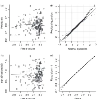
The functions that make up the kernel are statistical mod-els whose assumptions about the data can be assessed using standard model diagnostics. Statistical modelling choices are often based on tradition, such as logistic regression for survival. But tradition is often a reflection of what was computationally feasible many decades ago. Modern computers (and the advent of R) give us much more flexibility to let the data dictate the form of demo-graphic models and to carefully test the adequacy of sim-ple models. Figure 4 shows a few simsim-ple diagnostics for the Soay growth modelG(z′,z), again using the IBM artifi-cial data in the data framesim.data. The growth model is a linear regression, mod.grow < lm(z1 ∼ z, data = sim.data), here using a subset of the data so that growth is estimated from observations on about 190 indi-viduals. We also calculated the fitted values, residuals and standardized residuals, which will be used later:

zhat<- fitted(mod.grow)

resid<- residuals(mod.grow)

sresid<- rstandard(mod.grow)

The first three panels in Fig. 4 are similar to what you would get from R’s built-in diagnostics for a linear regres-sion usingplot(mod.grow). But we prefer to do it our-selves, so that we can use features from other packages (mgcv, car).

1 Residuals should have constant variance and no trend in mean; plotting residuals vs. fitted values

(panel a) provides a visual check on these properties. The plotted curve is a fitted nonparametric spline curve, using the gam function in the mgcv package (Wood 2011). It hints at the possibility of a small nonlinear trend, but this may be driven by a few points at the left (and since the data come from the IBM, we know that the underlying growth model really is linear).

2 Residuals should be Gaussian. A quantile–quantile plot (panel b), using the qqPlot function in the car library, supports this. Perfectly Gaussian residuals would fall on the 1 : 1 line (solid). The dashed lines are a 95% pointwise confidence envelope, so we should worry if more than 5% of points fall outside the envelope or if any points lie far outside it. In this case, the assumption that the residuals follow a Gauss-ian distribution seems reasonable. As a further check, we can test for statistically significant departures from Gaussian distribution:

shapiro.test(resid)

Shapiro–Wilk normality test

data: resid

W=0.9904, p-value=0.2438

This confirms what we know: the distribution of residu-als about the fitted growth curve is Gaussian.

3 A better check for constant error variance is a scale-location plot (panel c). The plotted points are the square root magnitude of the standardized residuals, Fitted values

Residuals

Normal quantiles

Residual quantiles

Fitted values

sqrt (|Residuals|)

2·8 2·9 3·0 3·1 3·2

2·8 2·9 3·0 3·1 3·2

−3 −2 −1 0 1 2 3

2·4 2·6 2·8 3·0 3·2

−0·2

−0·1

0·0

0·1

0·2

−2

−1

0

1

2

3

0·0

0·5

1·0

1·5

2·7

2·8

2·9

3·0

3·1

3·2

Size t

Fitted size t+1

(a) (b)

(c) (d)

Fig. 4. Diagnostic plots for the fitted Soay growth function. (a) Residuals vs. fitted values from the growth model. (b) Residual normal Q-Q plot. (c) Scale-loca-tion plot. (d) Expected size at t+1 under linear model (continuous line) and spline model (dashed line). See text for details. Source file: Ungulate Calcula-tions.Rin Supporting Information.

and the curve is again a fitted spline. The spline hints at a possible weak trend, so we test for correlation (using Kendall’s tau) but find none:cor.test(zhat, sqrt(abs(sresid)), method="k")givesP=040.

4 To follow-up on the hint of nonlinearity in panel (a), we can compare the linear model with a spline fit to the same data (panel d, solid and dashed lines).

The spline in panel (d) suggests that growth is a weakly nonlinear function of size. We know this is not true in this case – it is an accident of random sampling from a linear relationship –but with real data, we would have to decide between the linear and nonlinear models. The sta-tistical evidence is equivocal: a significance test using ano-va(mod.grow,gam.grow) is marginally non-significant (P=0089), while AIC slightly favours the nonlinear model (AIC=4116) over the linear model (AIC=4107).

The AIC difference is small enough that most users would probably select the simpler model. However, its lower AIC means that the nonlinear model is expected to make more accurate predictions (recall that in the frequ-entist framework AIC is a large-sample approximation to the out-of-sample prediction error, which is why frequen-tists and agnostics guiltlessly use both AIC and signifi-cance tests). Moreover, Dahlgren, Garcia & Ehrlen (2011) have shown that even weak nonlinearities can sometimes have substantial effects on model predictions, so the non-linear model should be taken seriously. When the statisti-cal evidence for one model over another is equivostatisti-cal, unless one of the models is strongly favoured based on some underlying biological hypothesis, we believe that the best approach is to try both models and attach most con-fidence to conclusions that the models agree on. Model averaging is another possibility, but current model averag-ing approaches are not always effective (Richards,

Whittingham & Stephens 2011) and we think that it is often more informative to show the degree of uncertainty by presenting the different results for the range of plausi-ble models.

In an IPM growth model, the residuals are just as important as the mean. In a typical regression analysis, the goal is to estimate the trend represented by the regres-sion line, and inference based on the model will be robust providing the residuals are ‘close enough’ to Gaussian, and the variance is ‘close enough’ to constant. But in an IPM, the scatter around the regression line for growth is also an important part of the model. A smaller growth variance in large individuals might be important for pre-dicting longevity because it keeps big individuals from shrinking, even if it is inconsequential for estimating the effect of size on mean growth rate.

Residual plots are less informative for the survival or probability of reproduction models, because all observed values are either 0 or 1, and there is no expectation of Gaussian residuals. One visual check is to compare model predictions with survival rates within size classes (Fig. 5a). And we can again compare the linear model with a non-linear model using gam (Fig. 5b). In this case, the linear model is supported: it has lower AIC, and the difference between the linear and nonlinear models is minuscule. Further checks are to test for overdispersion and to test whether the fit is significantly improved by adding predic-tors other than size (e.g. age).

i m p l e m e n t a t i o n : s i z e r a n g e a n d m e s h p o i n t s

It seems natural that a model’s size range should corre-spond to the range of observed sizes, perhaps extended a bit at both ends. Many published studies have used this approach. In our Soay example, we presented a ‘data’

Size z

Survival probability

2·0 2·4 2·8 3·2 2·0 2·4 2·8 3·2

0·0

0·2

0·4

0·6

0·8

1·0

–6

–4

–2

0

2

Size z

Spline (z, edf = 1)

(a) (b)

analysis based on a sample of 3000 observations. The min-imum and maxmin-imum observed sizes in this sample were 18 and 35, respectively. Because size is on a natural log scale, setting [L,U]=[16,37] allows the IPM to include individuals∼20% smaller or larger than any in the sam-ple. However, it is important to check whether a size range chosen in this sort of way is really big enough that individ-uals are not getting ‘evicted’ from the model. Eviction refers to situations where the distribution of subsequent sizez’ extends beyond [L,U], so that individuals in the tails of the growth distribution are not accounted for when the model is iterated (Williams, Miller & Ellner 2012).

An effective way to evaluate whether significant evic-tion is occurring via recruitment or survival-growth is to calculate the probability of eviction as a function of initial size. For example, in the Soay model, the probability that an established sizezindividual gets evicted is the integral of s(z)G(z′,z) from z′=U to z′=∞. Ideally, this number should be at most a fraction of a per cent for allz. What should you do if it is not? Or if you are worried that evic-tion might still affect evoluevic-tionary analyses, because it causes reproductive value to be underestimated? Unfortu-nately, there is no universally appropriate cure for evic-tion. A good starting point is to re-examine your growth model, as noted above. If eviction is happening because your growth model has an upper tail that extends beyond what is actually possible, a distribution with tighter limits on growth might fit the data better (e.g. a beta or trun-cated Gaussian distribution). If your growth model does not have an upper tail beyond z′=U but eviction is still occurring, there are several solutions you can try. These are discussed by Williams, Miller & Ellner (2012) so we will not review them here. As always, it is important to consider alternative assumptions and how those affect your conclusions.

Choosing the number of mesh points is a matter of bal-ancing accuracy against computation speed. The number of mesh pointsmrequired for accurate results depends on the kernel. An integral computed by mid-point rule will be accurate if the function being integrated is close to lin-ear on intervals of length h=(UL)/m. For IPMs, this means thathneeds to be small compared to the standard deviation of offspring size and to the standard deviation of growth incrementsz′z. If neither of these is too small, then a simple but effective approach is to start with a rea-sonable value ofm, say 50, and increase it until numerical results stabilize to the accuracy you need. But if either the standard deviation of offspring size or the growth incre-ments z′z is small, direct application of mid-point rule might lead to a very large matrix and to calculations that run slowly or crash when memory runs out.

Small variance in growth increments is particularly problematic. In practice, it arises for long-lived, slow-growing species. One option then is to use computational methods that can deal with large matrices. For example, the dominant eigenvalue and corresponding eigenvectors can be found without also calculating all the others as

eigendoes. Ellner & Rees (2006) explain how to do this by iteration, and Dawsons (2013) explains how to do this by calling ARPACK routines from within R. A second option is to use more accurate numerical integration methods (Dawson 2013). The third, and likely best, option is to use methods for sparse matrices. Linear alge-bra functions for sparse matrices (such as those in R’s spam and Matrix libraries) only store and work with the nonzero entries in a matrix. When growth is slow and nearly deterministic, the IPM kernel will be structured like a Leslie matrix, with zero or tiny values except in a small strip near the top (fecundity) and just below the diagonal (survival). Zeroing out transitions that do not really occur (e.g. if h*K[j,i]<109) will result in a very sparse matrix, and using sparse matrix methods will speed up the computations enormously. Sparse matrix methods can also be useful in more complex models where individ-uals are cross-classified by multiple traits (Ellner & Rees 2006).

Fitting more flexible demographic models

In the Soay example, we have assumed that all demo-graphic processes can be described by simple parametric models, indeed all the models fitted were linear or general-ized linear models with constant variance. Many empirical applications of IPMs have found these models to be ade-quate, but some cases need more flexibility. In this section, we briefly tour some useful approaches, going from simple (variable transformation) to complex (nonparametric esti-mates of growth variability) but without the need for com-plex coding by the user. To be concrete, we will think about parameterizing a growth kernel G(z′,z) depending only on individual size, by specifying the conditional mean m(z) =E[z′|z] and the pattern of individual variation around the mean. In a sense, this is just regression analy-sis, but as we noted above, it is also important to carefully model the between-individual variation in growth.

t r a n s f o r m i n g v a r i a b l e s

One long-standing approach is to seek a variable transfor-mation such that the transformed data are fitted by a sim-ple linear model. Log transformation is one examsim-ple, and it has been sufficient in many IPMs to date. When that fails, a power transformation is sometimes effective, z=xk where x is the raw size measurement (e.g. Bruno et al. 2011). Maximum likelihood can be used to find a good value ofk. For the linear modelyka+bxk+ Nor-mal(0,r2) with x,y,k>0, the profile negative log-likelihood ofkis (Box & Cox 1964, p. 215)

bcNLL=function(lambda,x,y){

xl<- x^lambda; yl<- y^lambda;

fit<- lm(yl_{xl); s2hat<- mean(fit$residuals^2);}

return(0.5*length(x)*log(s2hat/lambda^2)

(lambda-1)*sum(log(y)));

In the following test case, artificial data are created for whichz ¼ pffiffiffixfollows a standard linear regression model: z<- runif(N,1,10); z1<- 1+0.5*z+0.2*rnorm(N);

x<- z^2; x1<- z1^2;

To estimatek, we minimizebcNLLwithx=size in yeart, y=size in yeart+1,

lambdaHat<- optimize(bcNLL,c(0.01,3),x=x,y=x1)

$minimum

This givesk close to 05, as it should (mean=0495 and 90% of values between 037 and 062 with N=100 data points). The code is BoxCoxExample.R. Note, this is not equivalent to the boxcox function in R’s MASS library, which transforms only the dependent variable. In an IPM growth kernel, the independent variable is also size.

If a transformed variable is used in the growth kernel, it is simplest to use that transformation for the entire model. However, other demographic models can still be fitted on other scales. For example, letxbe measured size, and suppose that a growth kernel is fitted for z= logx but survival is fitted well by logistic regression on untrans-formed size, logit(s(x))=a+bx. The survival function on log scale is then logit(s(z))=a+bez. Transforming growth and offspring size models to different scales is also possi-ble but a bit more complicated, see Appendix 1.

n o n - c o n s t a n t v a r i a n c e

In many cases, a linear model has been adequate for the conditional mean (expected size next year), but the vari-ance in growth is not constant. This variability needs to be modelled so that the IPM produces realistic individual growth trajectories and size distributions.

Linear regression with several different size-dependent variance functions can be done in R usinggls(e.g. Ellner & Rees 2006). However, any variance function can be fit-ted by maximum likelihood. For example, if the mean and standard deviation of z0 are both linear functions of z, the negative log-likelihood is

-sum(dnorm(z1,mean=a+b*z,sd=c+d*z,log=TRUE)) and the parameter values can be estimated by mle in stats4. Even if your preferred model is available ingls or elsewhere, maximum likelihood has advantages. You can assume a non-Gaussian distribution for growth by substituting a different probability density for dnorm, such as a t distribution to accommodate fatter tails. And it is then easy to compare models of varying complexity using AIC, BIC or likelihood ratio tests (e.g. constant vs. linear vs. quadratic dependence on individual size).

n o n l i n e a r g r o w t h : m o d e l l i n g t h e m e a n

If your data cannot be transformed so that mean size at the next census is a linear function of present size, a non-linear mean function (such as a polynomial) can also be fitted by maximum likelihood. But unless you have some biological basis for specifying a particular nonlinear mean function, it is probably preferable to instead fit a flexible

nonlinear model whose shape is dictated by the data. This is a strength of R, and many options are available. If the variance appears to be constant, thegamfunction inmgcv can fit a spline whose degree of nonlinearity is automati-cally chosen based on the data. For the Soay data, all this takes are

require(mgcv); gamGrow<- gam(z1∼s(z),

data=sim.data)

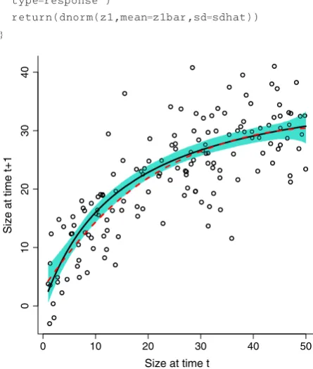
Note thats(z)in the line above is how the mean is spec-ified to be a spline function of z, not the survival func-tion. Figure 6 illustrates that this works surprisingly well with a moderate amount of data despite high variance about the mean.

The residuals from the fitted mean curve provide an estimate of the growth distribution’s standard deviation, sse<- sum(resid(gamGrow)^2);

sdhat<- sqrt(sse/df.resid(gamGrow));

In 1000 replicate simulated data sets with the same structure as in Fig. 6 and r=5, the mean estimate ofr was 498 and 90% of estimates were between 45 and 55.

There is no formula for the fitted mean function, but it still can be used in an IPM by using thepredictmethod forgammodels, as follows.

Gz1 z<- function(z1,z){

Gdata<- data.frame(z=z);

z1bar<- predict(gamGrow,newdata=Gdata,

type=response")

return(dnorm(z1,mean=z1bar,sd=sdhat)) }

0 10 20 30 40 50

01

0

2

0

3

0

4

0

Size at time t

Size at time t+1

Fig. 6. Example of fitting a nonlinear mean growth function with

n o n l i n e a r g r o w t h : p a r a m e t r i c v a r i a n c e

m o d e l s

Unfortunately, one data set can have several different complications. In the growth model just above, the mean function can be any smooth function, but the residuals are Gaussian with constant variance. It is still essential to check whether growth variability really fits that assump-tion and to improve the model when it does not.

Size-dependent variance and many non-Gaussian distri-butions can be fitted using the gamlss package. The mean, variance and up to two additional shape parame-ters can be fitted as either parametric or nonparametric functions of the independent variables. We cannot review all the options here, but we give one example to illustrate the possibilities. Suppose the growth variability in the last example is instead at distribution with d.f.=5 and non-constant variance. R’srtfunction generates a standardt distribution with variancer2

d:f: ¼ d.f.=ðd.f.2Þ, so below we use az-dependent factorscaleto create artificial size data with size-dependent variance in growth:

z<- runif(250,1,50)

# uniform distribution on [1,50]

z1bar<- 40*z/(15+z); scale<- 4*exp(-0.5+z/50);

z1<- z1bar+scale*rt(250,df=5)>

Figure 7 shows results from fitting these ‘data’, estimat-ing d.f. (assumed to be size-independent), a nonparametric mean function (cubic splines) and either a nonparametric

r(z) (cubic splines) or the truer(z) function (loglinear). The key point is that nonparametric fitting ofr(z) was almost as

good as (somehow) knowing the true functional form. The only cost is a slightly higher risk of missing the fat tails in the growth distribution (i.e. estimating d.f.≫5, Fig. 7c).

n o n p a r a m e t r i c v a r i a n c e m o d e l s

As a final level of generality, it is not even necessary to specify a distribution for the growth variability. This may be essential if no standard distribution can capture all the features evident in the growth data, or it may let you avoid a difficult choice between several candidates for the ‘right’ distribution.

Kernel density estimates are convenient for this because they are easy to use in an IPM growth kernel. The fitted den-sity function is just the average of a set of probability densi-ties (typically Gaussian) centred at the residuals. The one subtle point is that replacing each residual by a probability density increases the growth variance, so the residuals should be shrunk to offset this. This sounds complicated, but the code is simple.

For simplicity, we go back to constant variance, using gamto estimate the mean function. The first step is using the residuals to estimate the growth variance:

Resids<- resid(gamGrow); # extract residuals

sse<- sum(Resids^2); # sum of squared errors

sdhat<- sqrt(sse/gamGrow$df.residual)

# estimated Std Dev

The only thing we need from the kernel density estimate is its bandwidthh, the standard deviation of the probability densities centred at each residual:h<- bw.SJ(Resids);

Size at time t

Size at time t+1

Individual size

Growth standard deviation

pb(z) + pb(z) pb(z) + z

5 10 15 20

0 10 20 30 40 50 0 10 20 30 40 50

0

1

02

03

04

05

0

34

5

6

51

0

1

5

2

0

Estimated df, true sd function

Estimated df, spline sd function

(a)

(c)

(b)

Fig. 7. Simultaneously fitting the mean, variance and shape parameter of at distri-bution. (a) The solid black curve is the true mean function 40z/(15+z), and the circles are a typical data set. The dashed curves (red) are the pointwise 5th and 95th percentile estimates of the mean function across 250 simulated ‘data’ sets, using nonparametric splines (functionpb

in gamlss) for the mean and standard deviation functions. The nearly identical dotted curves (blue) are the same, but result from using the correct parametric form of the standard deviation. (b) The solid black curve is the true standard deviation; the dashed and dotted curves are pointwise 5th and 95th percentiles, as in panel (a). (c) Estimates of the shape parameter d.f. in the

The estimated probability density for growth is then the average of Gaussian densities centred at the scaled residu-als,dfunin the code below:

alpha<- sdhat/sqrt(sdhat^2+h^2);

# shrinkage factor

hResids<- alpha*Resids

# shrinking the residuals

dfun<- function(z) mean(dnorm(z,hResids,h))

dfun<- Vectorize(dfun)>

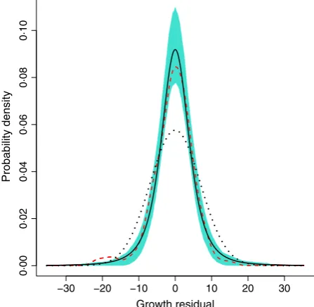
Figure 8 shows an example. The ‘data’ follow the model of Fig. 6 except that the growth variance was at distribu-tion with d.f.=3. Taking the pragmatic approach that the non-Gaussian error distribution will not throw off the esti-mate of the mean by much, we fitted the mean usinggam. The resultingdfunwas (correctly) markedly more peaked and fat-tailed than a Gaussian with the same standard deviation. But even with a decent amount of data (here, 150 data points), the estimate for an individual data set can be erratic, especially in the tails. So unless your data set is quite large, a nonparametric estimate of growth vari-ation is probably best used as an exploratory step to iden-tify the qualitative shape of the distribution. The final model can then use a parametric distribution (t, beta, log-normal, etc.) that has the right shape.

Kernels can still be used if the variance is size depen-dent. First, estimate the standard deviation function sdG and scale the residuals by their estimated standard

deviation, Resids <- resid(gamGrow)/sgG(z). Then compute h and hResids as above. The estimate of the growth distribution is then

dfun<- function(z) (1/sdG(z))*mean(dnorm(z/sdG

(z),mean=hResids,sd=h));

Again, this will only be reliable with a very large data set, because the scaled residuals depend on the estimated mean and standard deviation functions.

Recommendations and extensions

For the beginner just starting out building IPMs, we have two key recommendations:

Recommendation 1: Always draw a life cycle diagram like our Fig. 1, which summarizes the biology of the system, when the censuses occur, and has the demo-graphic functions indicated. Failing to do this can result in a model that does not represent your study system making any conclusions drawn difficult to jus-tify. We believe this is likely to be the commonest and most easily made mistake when starting out building IPMs and so recommend all publications using IPMs include a life cycle diagram like our Fig. 1 either in the main text or online.

Recommendation 2: Explore your model thoroughly using model diagnostics to test the model structure, whether the demographic models (s(z) etc) are appro-priate, and whether your conclusions are robust to the details of how the model is implemented (e.g. the size range and number of mesh points). We are great believers in ‘suck it and see’, so, for example, if your data does not unequivocally distinguish between two possible growth models then use both and compare the results. If you have used the code suggested in Section Implementing the IPM, exploring alternative growth models only involves changing the definition of G_z1z and rerunning your analysis. This approach to under-standing how the various assumptions influence your results will allow you to understand your system better and also determine which conclusions are robust and which need to be interpreted with caution.

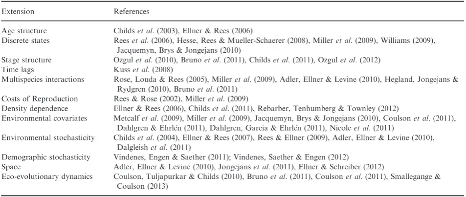
The simple IPM we have described is appropriate for some systems (e.g. Wallace, Leslie & Coulson 2013), but it will often be the case that the biology of the system will be more complicated. Since the introduction of IPMs (Easterling, Ellner & Dixon 2000), numerous extensions have been developed (Table 1). These extensions can be divided into two categories, those dealing with aspects of the environment in which the population occurs, dealing with say spatial or temporal variation in the quality envi-ronment, and those dealing with more complex life histo-ries, for example dormant states or stage structure where individuals are cross-classified by stage (e.g. juveniles and adults) and a continuous state (e.g. size). When building complex IPMs, our advice would be to start simple and add complexity when you are happy with your simpler

−30 −20 −10 0 10 20 30

0·00

0·02

0·04

0·06

0·08

0·10

Growth residual

Probability density