of visco-elastic fluid flows
C.-D. Tran1, D.-A. An-Vo,1N. Mai-Duy1and T. Tran-Cong1
Abstract: This paper presents a numerical approach for macro-micro multi-scale modelling of visco-elastic fluid flows based on the Integrated Radial Basis Function Networks (IRBFNs) and the Stochastic Simulation Technique (SST). The extra stress is calculated using the Brownian configuration fields (BCFs) technique while the velocity field is locally approximated at a set of collocation points using 1D-IRBFNs. In this approach, the stress is decoupled from the velocity field and computed from the molecular configuration directly without the need for a closed form rheological constitutive equation. The equations governing the macro flow field are discretised using a meshless collocation method where the IRBFN approximants improve the accuracy of the numerical solutions by avoiding the deterioration of accuracy caused by differentiation. As an illustration of the method, the time evolution of the planar Couette flow and the steady state Poiseuille flow are studied for two molecular kinetic models: the Hookean dumbbell and FENE dumbbell models.
Keywords: Integrated radial basis function networks, macro-micro multi-scale method, stochastic simula-tions, Brownian configuration fields, viscoelastic fluid.
1 Introduction
A common approach for the computation and analysis of complex fluid flows has been based on the coupling of the system of mass and momentum conservation equations with appropriate closed form constitutive equations. However, the disadvantage appears for some models which cannot be cast into closed form [e.g. Ottinger (1996); Bird, Armstrong, and Hassager (1987)]. Furthermore, in many complex fluids, rheological properties can only be captured at finer scales for the direct numerical simulation. A number of advanced numerical methods have been developed to appropriately deal with the above issues. Among these methods, the multi-scale methods [Engquist, Lötstedt, and Runborg (2000); Allaire and Brizzi (2005); Chu, Efendiev, Ginting, and Hou (2008); Hou (2005); Hajibeygi, Gonfigli, Hesse, and Jenny (2008)] have attracted significant attention for the last two decades. In this framework, the lack of information at the macroscopic level can be solved by a multiscale strategy consisting in searching for the information on the microstructures of the fluids. The information is then used to solve the macroscopic governing equations. This macro-micro multiscale approach does not require closed form constitutive equations [Ottinger (1996); Laso and Ottinger (1993); Feigl, Laso, and Ottinger (1995); Laso, Picasso, and Ottinger (1997); Hulsen, van Heel, and van den Brule (1997); Jourdain, Lelièvre, and Bris (2002)]. The approach is an attempt to emulate the situation in real liquids, where the full information about the stress is contained in the configuration of molecules which results from the micro-scale deformation history. The main idea of these techniques is that the polymer contribution to the stress is directly calculated from a large ensemble of microscopic configurations without having to derive a closed form constitutive equation, which is a powerful feature for the modelling of materials [Ottinger (1996); Engquist, Lötstedt, and Runborg (2000)].
Recently, the calculation of non-Newtonian flow by neural networks and stochastic simulation techniques [Tran-Canh and Tran-Cong (2002, 2004); Tran, Phillips, and Tran-Cong (2009)], which is based on a di-rect combination of the stochastic simulations and the differentiated radial basis function networks (DRBFNs) meshfree technique, was employed to model the hybrid systems. The present work is a further development of this approach with the incorporation of IRBFNs (instead of DRBFNs) and subdomain collocation (i.e.
1D-1Computational Engineering and Science Research Centre, Faculty of Engineering and Surveying, The University of Southern
IRBFNs) into the macro-micro approximation approach for solving non-Newtonian fluid problems. The pur-poses of using integration as a smoothing operator to construct the approximant are to avoid the reduction in convergence rate caused by differentiation and reduce the white noise in the approximation [Mai-Duy and Tran-Cong (2001)].
The paper is organised as follows. Section 2 gives a short review of the governing equations of incompress-ible non-Newtionian fluid flows using the macroscopic approach. In section 3, a macro-microscopic multi-scale modelling is described in which a stochastic simulation technique for the computation of the polymer-contributed stress is presented. Specifically, the coupled macro-micro multi-scale systems for the dumbbell models are introduced together with their non-dimensionalised forms. The discretisation of the coupled macro-micro models is detailed in section 4 where the BCFs and the 1D-IRBFN methods are described. An algorithm of the present procedure is presented to highlight the separate discretisations of the micro and macroscale com-ponents as well as their interaction. The numerical examples are then discussed in section 5 with a concludion in section 6.
2 Macroscopic governing equations for non-Newtonian fluid flows
Consider the isothermal flow of an incompressible fluid with density ρ, the system of mass and momentum conservation equations (governing PDEs) is given by
ρD
Dt(u) =−∇p+∇·τ, (1)
∇·u=0, (2)
where p, u are the hydrostatic pressure and velocity field respectively;τ the stress tensor defined by
τ=τs+τp, (3)
whereτs=2ηsD is the Newtonian solvent contribution; D (D=0.5(∇u+ (∇u)T)) the rate of strain tensor;ηs the solvent viscosity;τpthe polymer-contributed stress; and D/Dt(·)the substantial derivative defined by
D Dt(·) =
∂
∂t(·) + (u·∇)(·). (4)
For certain macroscopic models, it might be possible to obtain a closed form constitutive equation for the polymer-contributed stress(τp)in the form
Dτp Dt = f(τ
p,∇u). (5)
In the traditional approach, the conservation equations (1) and (2) are closed with a constitutive equation such as (5) involving the macroscopic quantities pressure, velocity and stress. In an alternative approach, the polymer-contributed stress can be calculated by directly solving appropriate stochastic differential equations governing the evolution of the microstructures of the polymer. Thus the coupling of the conservation equations (1) and (2) and the equations expressing evolution of the microscopic structures forms basis for the macro-microscopic multi-scale approach [Ottinger (1996); Bird, Armstrong, and Hassager (1987)]. Such a method is presented in the next section.
3 Macro-microscopic multi-scale modelling
3.1 The BCFs-based stochastic simulation technique
This technique is one of several potential approaches for analysis of complex fluids where the non-Newtonian character stems from the presence of micro-structures at a mesoscopic scale rather than at a real microscopic one. In this procedure, an appropriate equation describes the evolution of the micro-structures, and the non-Newtonian contribution τp to the stress is deduced from the evolving microstructures. In this context, the polymer chain is a linear arrangement of a number of non-interacting dumbbells. Each dumbbell consists of two Brownian beads with the friction coefficientζ, which are connected together by a spring. The configuration of a dumbbell is completely described by the length and orientation of the end-to-end vector R connecting the two beads [Ottinger (1996); Bird, Armstrong, and Hassager (1987)]. The state of the polymer chain is described by the set of R whose evolution are modelled using a stochastic differential equation (SDE) as follows [Hulsen, van Heel, and van den Brule (1997)].
dR(t,x) =
−u(t,x)·∇R(t,x) +∇u(t,x)·R(t,x)−2
ζF(R(t,x))
dt
+2
s
kBT
ζ dZ(t), (6)
where u is the velocity field;ζ the friction coefficient between the dumbbell and the solvent; kBthe Boltzmann constant; T the absolute temperature; Z(t) a standard multi-dimensional Brownian motion which is a Wiener process; F(R) is the internal force (also called spring force) exerted by a polymer in state R and depends on the kinetic model of the polymer. The coupling between the PDEs and SDE is carried out via the classical Kramers’ expression given by [Ottinger (1996); Bird, Armstrong, and Hassager (1987)]
τp=n
dhR⊗F(R)i −ndkBT Id, (7)
where nd is the density of dumbbells; I the identity tensor; d is the dimension of the ambient space; and ⊗ the tensorial product. With u(x)treated as a known macro field, the solution of the SDE (6) will yield R(t,x) which are then used to calculate the polymer-contributed stress. The stress (7) is then treated as known in the macro governing PDE (1). In SDE (6), the term u(t,x)·∇R(t,x)accounts for the convection of Brownian con-figuration fields by the flow. It can be seen that the existence of the convective term in this Eulerian framework [Hulsen, van Heel, and van den Brule (1997)] is completely equivalent to the particle tracking in the traditional Lagrangian CONNFFESSIT approach [Laso and Ottinger (1993)].
In this work, we consider the Hookean and Finitely Extensible Nonlinear Elastic (FENE) dumbbell models; and individual polymers as non-interacting dumbbells.
3.2 A coupled macro-micro multi-scale system
Collecting the partial differential conservation equations (1)-(2), the stochastic differential BCFs equations (6) and the Kramers’ expression (7) yields a macro-microscopic multi-scale system as follows.
ρ∂∂u
t +ρ(u·∇u)−η∆u+∇p=∇·τ
p, (8)
∇·u=0, (9)
dR=
−u·∇R+∇u·R−2
ζF(R)
dt+2
s
kBT
ζ dZ(t), (10)
τp=n
d(E(R⊗F(R))−kBT Id), (11)
the FENE model which plays an important role in non-linear rheological phenomena. The spring forces (F) of the Hookean and FENE dumbbell models are respectively given by
FHookean = RH,
FFENE =
RH 1− kRk2/(bk
BT/H) ,
where b is a non-dimensional parameter related to the maximal polymer length and H is a spring constant.
3.3 Non-dimensionalisation
Let U be a characteristic velocity;ηp=ndkBTλH the viscosity associated with the polymers;λH=ζ/4H the relaxation time of the polymer chains and L=pkBT/H the characteristic length scale [Ottinger (1996); Laso and Ottinger (1993); Jourdain, Lelièvre, and Bris (2002); Tran-Canh and Tran-Cong (2004)].
The dimensionless numbers Reynolds, Wissenberg andεare defined respectively as follows.
Re=ρU L
η ;We=λH
U L ;ε=
ηp
η ,
whereη(η=ηo+ηp) is the total viscosity of the solution. Thus, the macro-microscopic multi-scale system (8)-(11) is rewritten in the non-dimensionalised form as follows.
Re∂u
∂t +Re(u·∇u)−(1−ε)∆u+∇p=∇·τ
p, (12)
∇·u=0, (13)
dR=
−u·∇R+∇u·R− 1 2WeF(R)
dt+√1
WedZ(t), (14)
τp= ε
We(E(R⊗F(R))−Id), (15)
with F=FHookean=R and F=FFENE=(1−kRRk2/b)for the Hookean and FENE dumbbell models, respectively.
4 Discretisation of the macro-micro system using the multi-scale BCF-IRBFN method
In this section, the computational techniques are described for the numerical solution of micro-scale governing equations. The BCFs technique and the 1D-IRBFN collocation method are respectively presented for the discretisation of the SDEs and PDEs in the coupled macro-micro multi-scale system. The marriage of the two techniques to compute a macro-micro multiscale model is then presented in the overall algorithm.
4.1 Numerical solution of the SDEs
In this paper, the explicit Euler scheme is used for time dicretization of the SDE (14) for the Hookean dumbbell model and briefly presented as follows.
R(i+1)=Ri+
−ui·∇Ri+∇ui·Ri− 1
2WeF(Ri)
∆t+
r ∆t
WeZi, (16)
where Ri=R(ti);∆t is a fixed time step size for the stochastic process;∆Zi is normally distributed variable with expectation 0 and variance∆t and F(Ri)is defined as before. In the case of the FENE dumbbell model, the predictor-corrector method is employed to always satisfy the condition of a FENE dumbbell 0≤ |Qi+1|<√b.
More details of the method and its implementation for the Eulerian SDEs can be found in [Ottinger (1996); Tran-Canh and Tran-Cong (2004)].
Noise reduction issue is crucial in the stochastic simulation of systems such as (14). The variance reduction can be achieved by several techniques which are detailed in [Kloeden and Platen (1997); Gardiner (1994)]. In this work, the control variate method is employed for the dumbbell models. Details can be found in [Ottinger, van den Brule, and Hulsen (1997); Melchior and Ottinger (1996)], for example.
The method uses a control variatehRciwhich is correlated with the random variablehRi, to produce a better estimator ofhRi. WhilehRiis unknown and needs to be estimated,hRcican be calculated by a deterministic method. The control variate reduction technique is implemented as follows. At each collocation point, M dumbbells are assigned and numbered from i=1···M and dumbbells having the same index in the whole analysis domain have the same random number.
The implementation of the control variate technique for the dumbbell models can be found in, for example, [Bonvin and Picasso (1999); Tran-Canh and Tran-Cong (2004); Tran, Phillips, and Tran-Cong (2009)] and is not repeated here. Since dumbbells are processed at the collocation points, it is easy to incorporate the control variate technique in the present BCF-IRBFN collocation method.
4.2 The IRBFN collocation method for solving PDEs
Consider the conservation equations (12)-(13), reproduced here for convenience,
Re∂u
∂t +Re(u·∇u)−(1−ε)∆u+∇p=∇·τ p,
∇·u=0,
where τp is a known function obtained from the stochastic process in the coupled macro-micro multiscale system.
In order to solve the system of Eqs. (12)-(13), the problem domain is discretised using a set of nodal points, called the global macro-scale grid. In this work, instead of using the continuity equation (13), the incompress-ibility condition is enforced via the penalty method as follows [Feigl, Laso, and Ottinger (1995)].
p=−pe∇·u, (17)
where pe is a sufficiently large penalty parameter. Equation (12) is then rewritten as
Re∂u
∂t +Re(u·∇u)−(1−ε)∆u−pe∇(∇·u) =∇·τ
p. (18)
In this paper, the 1D-IRBFN scheme is employed to approximate spatial derivatives, whereas a finite difference technique is used for temporal discretisation.
4.2.1 Spatial discretisation
At a time t the domain under consideration is discretised using a uniform Cartesian grid. Let Nxand Nybe the numbers of grid lines in the x and y directions respectively. The dependent variables and their derivatives are approximated using a 1D-IRBFN interpolation scheme which is presented in the following sections.
a) 1D IRBFN scheme on a grid line: x and y directions
The variation of dependent variable u along an x-gridline in the IRBFN form [Mai-Duy and Tran-Cong (2007)] starts with
∂2u
∂x2 = Nx
∑
i=1 wigi=
Nx
∑
i=1 wiG[
2]
i , (19)
where{wi}Ni=x1is the set of RBF weights;{gi(x)}Ni=x1the set of Multi-quadric RBFs (MQ-RBFs) [Hardy (1971); Franke (1982); Kansa (1990)] and given by
gi(x) = (x−ci)2−a2i
1/2
, (20)
The corresponding first-order derivative and function are then determined through integration as follows
∂u
∂x = Nx
∑
i=1 wiG[
1]
i +C1, (21)
u= Nx
∑
i=1
wiG[i0]+C1x+C2, (22)
where Gi[1](x) =RG[i2](x)dx, Gi[0](x) =RG[i1](x)dx and C1and C2are unknown constants of integration. Collocating equations (19), (21) and (22) at a set of grid points {xi}Ni=x1 yields the following set of algebraic equations
g ∂2u
∂x2 =Ge
[2]we, (23)
f ∂u
∂x =Ge
[1]we, (24)
e
u=Ge[0]we, (25)
where
e
G[2]=
G[12](x1) G[22](x1) ··· G[N2x](x1) 0 0 G[12](x2) G[
2]
2 (x2) ··· G[ 2]
Nx(x2) 0 0
..
. ... . .. ... ... ... G[12](xNx) G
[2]
2 (xNx) ··· G
[2]
Nx(xNx) 0 0 , e
G[1]=
G[11](x1) G[ 1]
2 (x1) ··· G[ 1]
Nx(x1) 1 0
G[11](x2) G[21](x2) ··· G[N1x](x2) 1 0
..
. ... . .. ... ... ... G[11](xNx) G
[1]
2 (xNx) ··· G
[1]
Nx(xNx) 1 0 , e
G[0]=
G[10](x1) G[20](x1) ··· G[N0x](x1) x1 1
G[10](x2) G[20](x2) ··· G[N0x](x2) x2 1 ..
. ... . .. ... ... ... G[10](xNx) G
[0]
2 (xNx) ··· G
[0]
Nx(xNx) xNx 1 , e
w = (w1,w2,···,wNx,C1,C2) T,
e
u = (u1,u2,···,uNx) T
, g
dku dxk =
dku1 dxk ,
dku2 dxk ,···,
dkuNx
dxk
T
,
where ui=u(xi)with i= (1,2,···,Nx).
Owing to the presence of integration constants of the IRBFN based approximation, one can beneficially intro-duce in the algebraic equation system additional constraints such as nodal derivative values (more details can be found in [Mai-Duy and Tran-Cong (2007)]). Thus, the algebraic equation system (25) can be reformulated
as follows. e u e f = " g
G[0]
e
L
# e
w=Cewe,
where ef =eLw are additional constraints. The conversion of the network-weight space into the physical spacee yields
e
w=Ce−1
e
C−1is the conversion matrix. By substituting (26) into (19) and (21), the second and first-order derivatives of u will be expressed in terms of nodal variable values as follows.
∂2u
∂2x =D2xu˜+k2x,
∂u
∂x =D1xu˜+k1x,
(27)
whereD1xandD2xare known vectors of length Nx; and k2xand k1xscalars and determined by ef . Applying (27) at each and every collocation point on the gridline yields
f
∂2u
∂2x =De2xu˜+ek2x,
f∂u
∂x =De1xu˜+ek1x,
(28)
whereDe2xandDe1xare known matrices of dimension Nx×Nx; andek2x andek1x are known vectors of length Nx. Similarly, along a y-gridline, the values of the second and first order derivatives of u in the IRBFN form at all collocation points can be expressed by
f
∂2u
∂2y =De2yu˜+ek2y,
f∂u
∂y =De1yu˜+ek1y,
(29)
whereDe2yandDe1yare known matrices of dimension Ny×Ny; andek2yandek1yare known vectors of length Ny. b) 1D-IRBFN scheme on 2D computational domain
The second and first order and cross derivatives of u with respect to x and y over the whole domain can be expressed using Kronecker tensor products as
d ∂2u
∂x2 =
e
D2x⊗Iy
ˆ
u+ˆk2x=Db2xuˆ+ˆk2x, (30)
c ∂u
∂x =
e
D1x⊗Iy
ˆ
u+ˆk1x=Db1xuˆ+ˆk1x, (31)
d ∂2u
∂y2 =
Ix⊗De2y
ˆ
u+ˆk2y=Db2yuˆ+ˆk2y, (32)
c ∂u
∂y =
Ix⊗De1x
ˆ
u+ˆk1y=Db1yuˆ+ˆk1y, (33)
d ∂2u
∂x∂y = 1 2
b
D1xDb1y+Db1yDb1xuˆ+ˆk2xy, (34)
whereDb2x,Db1x,Db2y,Db1yandDb2xyare known matrices of dimension NxNy×NxNy; ˆk2x, ˆk1x, ˆk2y, ˆk1y ˆk2xy known vectors of length NxNy; ˆu= (u(1),u(2), . . . ,u(NxNy))T;⊗the tensorial product; and Ixand Iythe identity matrices of dimension NxNxand NyNy, respectively.
All boundary conditions are directly imposed on the IRBFN approximations, and the governing equations are forced to be satisfied locally on each and every gridline. Further details of the method will be described through the numerical examples in section 5.
4.2.2 Time discretisation
For transient problems, the fully implicit Euler method is employed for the temporal discretisation.
4.3 Algorithm of the present procedure
(a) Generate a set of collocation points. Start with a given initial condition for the first iteration (velocity field, molecular configurations) together with the given boundary conditions of the problem. In the present work, the initial conditions are zero initial velocity field, and initial molecular configurations sampled from equilibrium Gaussian distribution (e.g. [Tran-Canh and Tran-Cong (2002, 2004)]);
(b) Assign M dumbbells to each collocation point. All dumbbells at a collocation point having the same index constitute a configuration. Hence, there is an ensemble of M configuration fields Ri (i=1···M). Since
all the dumbbells having the same index receive the same random numbers, there is a strong correlation between dumbbells in a configuration. The control variates ˆRiassociated with the configuration fields Ri
are created [Bonvin and Picasso (1999); Tran-Canh and Tran-Cong (2004)];
(c) Solving the macro PDEs for the velocity field using the 1D-IRBFN collocation method described in section (4.2);
(d) Solving the micro SDEs for the polymer configuration fields using the method presented in section (4.1). As mentioned in step (a), in order to ensure strong correlation within a configuration field, all the dumbbells of the same index have the same random numbers. For each configuration field Ri, a corresponding control
variate is determined (see Tran-Canh and Tran-Cong (2004) for details);
(e) Determine the polymer contribution to stress by taking the ensemble average of the polymer configurations at each collocation point xi, using Eq. (15);
(f) With the stress field just obtained, solve the macro governing equations (12)-(13) for the new velocity field using the 1D-IRBFN method described in section (4.2);
(g) Terminate the simulation when either the desired time or convergence is reached. The latter is determined by a convergence measure (CM) for the velocity field, defined by
CM(u) =
v u u
t∑N1 ∑di=1 uni −uni−1
2
∑N
1∑di=1(uni)2
≤tol (35)
where d is the number of dimensions; tol a preset tolerance; ui the i-component of the velocity at a collo-cation point; N the total number of collocollo-cation points and n the iteration number.
(h) Return to step (d) for the next time step of the microscopic process until steady state or a given time is reached.
5 Numerical examples
The present method is verified with the simulation of the start-up planar Couette flow of Hookean and FENE dumbbell fluids and the steady state planar Poiseuille flow of Hookean dumbbell fluids.
5.1 Start-up planar Couette flow using the dumbbell models
This problem was earlier studied by [Laso and Ottinger (1993); Mochimaru (1983); Tran-Canh and Tran-Cong (2002, 2004)], and it is used here to verify the present method for the Hookean and FENE dumbbell models. The problem is defined in Fig. 1. For time t<0, the fluid is at rest. At t=0, the lower plate starts to move with a constant velocity V =1. No-slip condition is assumed at the walls.
From the characteristics of the start up Couette flow problem and a dumbbell model of polymer, the macro-micro system of equations (12)-(15) is rewritten as follows [Jourdain, Lelièvre, and Bris (2002)].
Re∂u
∂t(t,y)−(1−ε)
∂2u
∂y2(t,y) =
∂τp
∂y (t,y), (36)
dP(t,y) =
−2We1 FP(R(t,y)) +
∂u
∂y(t,y)Q(t,y)
dt+√1
dQ(t) =− 1
2WeFQ(R(t,y))dt+ 1 √
WedW(t), (38)
τp(t,y) = ε
We(E(P(t,y)Q(t)), (39)
where u andτpare the x-component of the velocity and the shear stressτxyp of the flow, respectively; (P, Q) and (V,W ) the components of a process R and two independent Brownian motions, respectively of a configuration of dumbbell at location y; and (FP,FQ) are two components of the force F(R).
The stochastic differential equations (37)-(38) are given by
dP(t,y) =
−2We1 P(t,y) +∂u
∂y(t,y)Q(t,y)
dt+√1
WedV(t), (40)
dQ(t) =− 1
2WeQ(t)dt+ 1 √
WedW(t), (41)
for the Hookean dumbbell model, and
dP(t,y) =
−2We1 ·1 P(t,y) − kRk2/b+
∂u
∂y(t,y)Q(t,y)
dt+√1
WedV(t), (42)
dQ(t) =− 1 2We·
Q(t,y)
1− kRk2/bdt+ 1 √
WedW(t), (43)
for the FENE dumbbell model, wherekRk2=P2(t,y) +Q2(t,y)and b is defined as before.
In this section, only the time discretisation of the Hookean dumbbell SDEs is described, and that for the FENE dumbbell model is similarly obtained. The discretisation of equations (36), (40)-(41) and (39) are carried out through two interlaced processes of different scales as follows.
5.1.1 Discretisation of the micro-scale stochastic governing equation
Eqs (40)-(41) are discretised using the Euler explicit scheme in time with M=1000 realizations of each random process as follows.
Pih+1,j=
1− ∆t 2We
Pih,j+
∂
uj
∂y
h
i+1
Qhi∆t+
r ∆t We∆V
h
i,j, (44)
Qhi+1=
1− ∆t 2We
Qhi +
r ∆t We∆W
h
i , (45)
where i and j are for the time and space discretisations, respectively; h (1≤h≤M) stands for the realisation of random processes; and∆Vih,j and∆Wihare standard normal random variables. The velocity field of the flow at the times ti is either given by the initial conditions or the solution of the macro-scale process which was previously determined using the 1D-IRBFN method. It is worthy of note that Qh are independent of their position y, owing to the simple geometry of problem.
The stressτpis then calculated using the coupling equation (39) as follows.
(τp)
i+1,j= ε We
1 M
M
∑
h=1
Pih+1,jQhi+1. (46)
The stresses (τp)
5.1.2 Discretisation of the macro-scale governing equation
Applying the full implicit method for time discretisation of the macro-governing equation (36) yields
Reui+1−ui
∆t −(1−ε)
∂2u i+1
∂y2 =
∂(τp) i
∂y , or
βui+1−α∂ 2u
i+1
∂y2 =
∂(τp) i
∂y +βui, (47)
where∆T is uniform time step;β =Re/∆t;α=1−ε; and ui+1=u(y,ti+1)with u0=u(y,0).
Since it is a 1D problem, the time discrete equation (47) is then spatially discretised using equation (29) (section 4.2). The spatial domain (0≤y≤1) is discretised using Nyuniform collocation points. T is the final time when the flow has reached its steady state.
• Initial conditions
u(0,0) =V =1; u(0,y) =0 ∀y6=0. (48)
• Dirichlet boundary conditions
u(t,0) =V=1 ∀t>0; u(t,L) =0 ∀t>0. (49)
The parameters of the problem are: Wissenberg number We=0.5, Reynolds number Re=0.1 and the ratio
ε=0.9.
Using the time step∆t=10−2for both macro and micro processes, a coarse spatial discretisation ∆y=0.05 (Ny=21) and number of dumbbells N=1000 at each collocation points, results by the 1D-IRBFNs collocation method are in good agreement with ones obtained from a macroscopic approach (Finite Difference Method) using Oldroyld-B model.
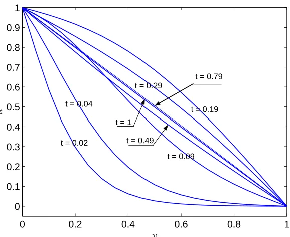
Figs. 2 and 3 show time evolutions of the velocity and shear stress respectively at four locations y=0.2, 0.4, 0.6 and 0.8. Fig. 4 describes the evolution of the velocity profile, which shows that velocity exhibits undershoot and overshoot before reaching the steady state at t=1.
Using a coarser number of collocation points (Ny=11,∆t=0.01) and (Ny=15,∆t=0.01), the results showed that the present method is able to produce a very high degree of accuracy using a relatively coarse grid.
The problem is also solved for the FENE dumbbell model using the present method with the following chosen physical parameters: ηo=ηN+ηp=1,ρ=1.2757,λH =49.62,ηN =0.0521 as done in [Laso and Ottinger (1993); Tran-Canh and Tran-Cong (2002, 2004)], whereηo,ηN,ηp,ρ,ηH andρN are defined as before.
The corresponding Wissenberg, Reynolds numbers and the ratioεare given by
Re=ρηV L
o =1.2757; We=
λHV
L =49.62 and ε=
ηp
ηo =0.9479.
For this case, the Predictor-Corrector method is employed to discretise the SDEs (42)- (43) as mentioned in section 4.1. Fig. 5 describes the evolution of the velocity profile, which shows that velocity overshoot is pretty clear. Figs 6 and 7 show the time evolution of the velocity and shear stress, respectively at four locations y=0.2, y=0.4, y=0.6 and y=0.8, using 21 collocation points. The results also show that velocity reaches the steady state sooner than the shear stress. The numerical solutions by the present method confirm a very good agreement with the results of other methods where finer meshes or collocation points [Laso and Ottinger (1993); Tran-Canh and Tran-Cong (2004)] were used.
5.2 Steady state Planar Poiseuille flow
In this example, the Hookean model is considered. The fluid parameters are chosen as in [Feigl, Laso, and Ottinger (1995); Tran-Canh and Tran-Cong (2004)]: the relaxation time is λH=1, the total viscosity η0=
ηN+ηp, the density of fluid ρ =1 and the ratio between the viscosity of solvent and polymer ηN/ηp=1. Thus, the corresponding Reynolds, Wissenberg numbers and the ratioε= ηp
ηo are given by
Re=ρhηuia
o =
2 3
ρVa
ηo =
2
3; We=λH hui
a = 2 3λH
V a =
2
3; andε=
ηp
ηo =0.5.
5.2.1 Coupled macro-micro governing equations for the Poiseuille flow
Together with the stochastic equations of the Hookean dumbbell model, the coupled macro-micro governing equations developed from Eq (18) for the case of steady fluid flow are given by
Re
u∂u
∂x+v
∂u
∂y
−α ∂2u
∂x2+
∂2u
∂y2
−Pe ∂2u
∂x2+
∂2u
∂x∂y
=∂τ p xx
∂x +
∂τp yx
∂y , (50)
Re
u∂v
∂x+v
∂v
∂y
−α ∂2v
∂x2+
∂2v
∂y2
−Pe ∂2v
∂x2+
∂2v
∂x∂y
=∂τ p xy
∂x +
∂τp yy
∂y , (51)
dR=
−u·∇R+∇u·R− R
2We
dt+√1
WedZ(t), (52)
τp= ε
We(E(R⊗R)−Id), (53)
where α = ηN
ηo =
ηo−ηp
ηo =1−ε; (u,v) are two components of velocity field u. For the Hookean dumbbell
(Oldroyd-B) model, the creeping Poiseuille flow problem has an analytical solution given by
τp
xx=3(1−α)We
∂
u
∂y
2
; τxyp = (1−α)∂u
∂y; τ
p
yy=0. (54)
The analytical solution is used to judge the quality of the following numerical simulation.
5.2.2 Boundary conditions
The macroscopic boundary conditions are given in dimensionless form as follows.
• Dirichlet boundary condition
- On the wall (Γ4): u(x,y) =0 and v(x,y) =0.
- At the inlet (Γ1) and outlet sections (Γ3), the flow is fully developed Poiseuille where the velocity profile is parabolic: u(x,y) = (1−y2); v(x,y) =0.
- On the centreline (Γ2): v(x,y) =0. • Neumann boundary condition
- On the centreline (Γ2): ∂∂uy =0.
5.2.3 Discretisation of the problem using the present method
While the SDEs are discretised using the explicit Euler scheme (see section 4.1) with 1000 dumbbells at each collocation point and micro time step size∆t=0.01, the conservation equations (50)-(51) are solved using the 1D-IRBFN method.
It can be seen that the RHS’s of the conservation equations are known and obtained from the solution of the SDE (52) and the coupling equation (53). Furthermore, the first derivatives of stresses in the RHS are also approximated using the IRBFN method.
The non-linear convective terms(u·∇)u in (50)-(51) are linearized using a Picard-type iterative procedure as follows: keep the derivatives as unknown, i.e.(u·∇)u is represented by(ui·∇)ui+1and the current estimate of velocity field as a known (the initial zero-value velocity field for the first iteration).
5.2.4 Results and discussion
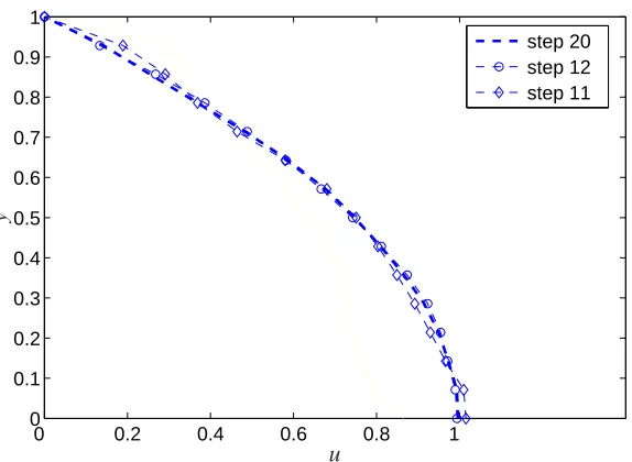
The obtained result shows that the parabolic velocity profile is accurately recovered in the whole domain as expected (Fig. 9). The figure describes the velocity profile on the middle plane x=0.5 with respect to y for the steps 11, 12 and 20. While the solution obtained for the velocity field quickly reaches the steady state after few iterations, shear stress and the first normal stress difference require about 200 iterations to reach the steady state. Fig. 10 shows the evolution of polymer shear stress and the first normal stress difference through several steps at the middle plane x=0.5 with respect to y.
The convergence measures (CM) for the shear stress and the first normal stress difference are around 10−3 -10−4and show that results obtained by the present method are in good agreement with the analytical solution given by Eq. (54).
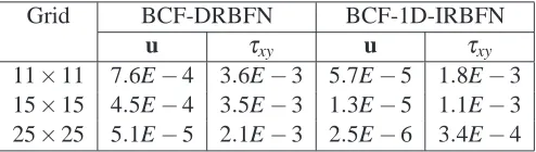
The problem is also solved using coarser grids of collocation points: (11×11) and (15×15). The results showed that the present method is able to produce a high degree accuracy using a relatively coarse grid, how-ever insufficient number of dumbbells at each collocation point will result in oscillatory behaviours even with variance reduction method. For example, when the number of dumbbells at each collocation point is reduced to 500, oscillatory behaviour sets in. The present results are also compared with those obtained by the BCF-DRBFN method [Tran-Canh and Tran-Cong (2004)]. It can be seen that the proposed BCF-1D-IRBFN method outperforms the BCF-DRBFN method regarding convergence (see Tab. 1).
Although further investigations are required, the preliminary results have shown that while the proposed BCF-1D-IRBFN method have significantly improved the accuracy of the velocity because it avoids the deterioration of accuracy caused by differentiation in both SDEs and PDEs. The improvement of the shear stress is more modest due to the stochastic nature of the microscopic stress calculation.
6 Conclusion
This paper reports the development of a macro-micro multi-scale method for the computation of visco-elastic fluid flows using a combination of the 1D-IRBFN method and the Eulerian stochastic simulation technique. The advantages of the present approach include (i) to obviate the need for a closed form constitutive equation as well as particle tracking for micro-scale processes; (ii) to yield a meshless discretisation of governing equations; (iii) to improve the approximation accuracy by avoiding the reduction in convergence rate caused by differentiation; and (iv) to reduce the white noise in the approximation via the use of integration as a smoothing operator to construct the approximants. The method is verified with standard test problems, namely the start up Couette flow and the planar Poiseuille flow problems.
Acknowledgement: This work was supported by the Australian Research Council.
References
Allaire, G.; Brizzi, R. (2005): A multiscale finite element method for numerical homogenization. Multiscale Modeling & Simulation, vol. 4, pp. 790–812.
Bird, R. B.; Armstrong, R. C.; Hassager, O. (1987): Dynamics of polymeric liquids, V.2. John Wiley & Sons:New York.
Bonvin, J.; Picasso, M. (1999): Variance reduction methods for connffessit-like simulations. Journal of Non-Newtonian Fluid Mechanics, vol. 84, pp. 191–215.
Chu, J.; Efendiev, W.; Ginting, V.; Hou, T. Y. (2008): Flow based over-sampling technique for multiscale finite element methods. Advances in Water Resources, vol. 31, pp. 599–608.
Engquist, B.; Lötstedt, P.; Runborg, O. (2000): Multiscale Methods in Science and Engineering: Lecture Notes in Computational Science and Engineering V. 44. Springer:Berlin.
Franke, R. (1982): Scattered data interpolation: tests of some methods. Mathematics of Computation, vol. 38, pp. 181–200.
Gardiner, C. W. (1994): Handbook of Stochastic Methods for Physics, chemistry and the natural Sciences. Springer:Berlin.
Hajibeygi, H.; Gonfigli, G.; Hesse, M. A.; Jenny, P. (2008): Iterative multiscale finite-volume method. Journal of Computational Physics, vol. 227, pp. 8604–8621.
Hardy, R. L. (1971): Multiquadric equations for topography and other irregular surfaces. Journal of Geophysical Research, vol. 76, pp. 1905–1915.
Haykin, S. (1999): Neural networks: A comprehensive foundation. New Jersey:Prentice Hall.
Hou, T. Y. (2005): Multiscale modelling and computation of fluid flow. International Journal for Numerical Methods in Fluids, vol. 47, pp. 707–719.
Hulsen, M. A.; van Heel, A. P. G.; van den Brule, B. H. A. A. (1997): Simulation of viscoelastic flow using brownian configuration fields. Journal of Non-Newtonian Fluid Mechanics, vol. 70, pp. 79–101.
Jourdain, B.; Lelièvre, T.; Bris, C. L. (2002): Numerical analysis of micro-macro simulations of polymeric fluid flows: a simple case. Mathematical Models and Methods in Applied Sciences, vol. 12, pp. 1205–1243.
Kansa, E. (1990): Multiquadrics-a scattered data approximation scheme with applications to computational fluid-dynamics-i: Surface approximations and partial derivatives estimates. Computers & Mathematics with Applications, vol. 19, pp. 127–145.
Kloeden, P. E.; Platen, E. (1997): Numerical solution of stochastic differential equations. Springer:Berlin.
Laso, M.; Ottinger, H. C. (1993): Calculation of viscoelastic flow using molecular models: the connffessit approach. Journal of Non-Newtonian Fluid Mechanics, vol. 47, pp. 1–20.
Laso, M.; Picasso, M.; Ottinger, H. C. (1997): 2-d time-dependent viscoelastic flow calculation using connffessit. AIChE Journal, vol. 43, pp. 877–892.
Mai-Duy, N.; Tran-Cong, T. (2001): Numerical solution of Navier-Stokes equations using multiquadric radial basis function networks. International Journal for Numerical Method in Fluids, vol. vol. 37, pp. 65–86.
Mai-Duy, N.; Tran-Cong, T. (2007): A collocation method based on one-dimensional rbf interpolation scheme for solving pdes. International Journal of Numerical Methods for Heat & Fluid Flow, vol. 26, pp. 426–447.
Melchior, M.; Ottinger, H. C. (1996): Variance reduced simulations of polymer dynamics. Journal of Chemical Physics, vol. 105, pp. 3316–3331.
Mochimaru, Y. (1983): Unsteady-state development of plane couette flow for viscoelastic fluids. Journal of Non-Newtonian Fluid Mechanics, vol. 12, pp. 135–152.
Ottinger, H. (1996): Stochastic processes in Polymeric Fluids. Springer:Berlin.
Ottinger, H. C.; van den Brule, B. H. A. A.; Hulsen, M. A. (1997): Brownian configuration fields and variance reduced connffessit. Journal of Non-Newtonian Fluid Mechanics, vol. 70, pp. 255–261.
Tran, C. D.; Phillips, D. G.; Tran-Cong, T. (2009): Computation of dilute polymer solution flows using bcf-rbfn based method and domain decomposition technique. Korea Autralia Rheology Journal, vol. 21, pp. 1–12.
Table 1: CM for the velocity field and shear stress obtained by the BCF-DRBFN [Tran-Canh and Tran-Cong (2004)] and BCF-1D-IRBFN methods for several grid sizes at the step 220 after reaching the steady state, using 1000 dumbbells at each nodal point and micro-time step size∆t=0.01.
Grid BCF-DRBFN BCF-1D-IRBFN
u τxy u τxy
11×11 7.6E−4 3.6E−3 5.7E−5 1.8E−3 15×15 4.5E−4 3.5E−3 1.3E−5 1.1E−3 25×25 5.1E−5 2.1E−3 2.5E−6 3.4E−4
[image:15.595.184.418.428.632.2]0 0.2 0.4 0.6 0.8 1 0
0.2 0.4 0.6 0.8 1
y = 0.2
y = 0.4
y = 0.8 y = 0.6
u
[image:16.595.163.456.87.325.2]t
Figure 2: Start-up planar Couette flow problem (Fig. 1) using the Hookean dumbbell model: the parameters of the problem are number of dumbbells N=1000, number of collocation points M=21,∆t=0.01, Wissenberg Number We=0.5, Reynolds number Re=0.1 and the ratio ε =0.9. The time evolution of the velocity at locations y=0.2, y=0.4, y=0.6 and y=0.8.
0
0.2
0.4
0.6
0.8
1
0
0.2
0.4
0.6
0.8
y = 0.2
y = 0.40
y = 0.60
y = 0.80
−
τyx
t
0 0.2 0.4 0.6 0.8 1 0
0.1 0.2 0.3 0.4 0.5 0.6 0.7 0.8 0.9 1
t = 0.02 t = 0.04
t = 0.09 t = 0.19 t = 0.29
t = 0.49
t = 0.79
t = 1
u
y
Figure 4: Start-up planar Couette flow problem using the Hookean dumbbell model: the parameters of the problem are shown in Fig. 1 and the caption of Fig. 2. The velocity profile with respect to location y at different times.
0 0.2 0.4 0.6 0.8 1
0 0.1 0.2 0.3 0.4 0.5 0.6 0.7 0.8 0.9 1
t = 0.30
t = 0.50 t = 0.90
t = 1.20
t = 1.60
t = 2.00 t = 2.50
t = 3.00 t = 3.50 t = 4.00 t = 5.00
t = 5.50
u
(
y
,
t
)
[image:17.595.165.454.91.327.2]y
0 1 2 3 4 5 6 0
0.1 0.2 0.3 0.4 0.5 0.6 0.7 0.8 0.9 1
y = 0.0 y = 0.4 y = 0.6 y = 0.8
u
t
Figure 6: Start-up planar Couette flow problem using the FENE dumbbell model: the parameters of the problem are shown in Fig. 1 and the caption of Fig. 5. The time evolution of the velocity at locations y=0.2, y=0.4, y=0.6 and y=0.8.
0 10 20 30 40
0 0.1 0.2 0.3 0.4 0.5
0.6 y = 0.2
y = 0.4 y = 0.6 y = 0.8
−
τyx
t
Figure 8: Steady planar Poiseuille flow problem: a) Parabolic inlet velocity profile; non-slip boundary condi-tions applied at the fluid-solid interfaces. b) The collocation point distribution is only schematic.
0 0.2 0.4 0.6 0.8 1 0
0.1 0.2 0.3 0.4 0.5 0.6 0.7 0.8 0.9 1
step 20 step 12 step 11
u
y
[image:19.595.167.454.432.642.2]0 0.2 0.4 0.6 0.8 1 −0.8
−0.6 −0.4 −0.2 0 0.2 0.4 0.6 0.8 1 1.2
Φ1
τyx
[image:20.595.153.457.77.339.2]y
Figure 10: Steady state planar Poiseuille flow problem using the Hookean dumbbell model: the polymer shear stress and the first normal stress difference on the middle plane x=0.5 with respect to y for several initial steps.
0 0.2 0.4 0.6 0.8 1
−1 −0.5 0 0.5 1 1.5 2 2.5 3 3.5 4
Approximated solution Analytical solution Φ1
τyx
y
[image:20.595.154.457.420.694.2]