A method of optimal image subtraction: development of the mathematics and software for general use in astronomical research

Full text

(1)A METHOD OF OPTIMAL IMAGE SUBTRACTION Development of the Mathematics & Software for General Use in Astronomical Research J. Patrick Miller A thesis submitted for the degree of Doctor of Astronomy at the Centre for Astronomy James Cook University, Townsville. July, 2008. 1.

(2) Statement of Access. I, the undersigned, author of this work, understand that James Cook University will make this thesis available for use within the University Library and, via the Australian Digital Theses network, for use elsewhere. I understand that, as an unpublished work, a thesis has significant protection under the Copyright Act and; I do not wish to place any further restriction on access to this work.. Signature. 2. July 31, 2008 Date.

(3) Statement of Sources. DECLARATION I declare that this thesis is my own work and has not been submitted in any form for another degree or diploma at any university or other institution of tertiary education. Information derived from the published or unpublished work of others has been acknowledged in the text and a list of references is given.. Signature. 3. July 31, 2008 Date.

(4) Statement of Contributions of Others This thesis describes work carried out for the Centre for Astronomy at James Cook University, Townsville (Australia). As an Internet-based international student, I have never been on the Townsville campus but have done all of my work at Hardin-Simmons University where I am an associate professor of mathematics and at the Lawrence Berkeley National & Space Sciences Laboratory (University of California, Berkeley) under the direction of my advisor Dr. Carlton R. Pennypacker. Sections 1.2 and 1.3 in Chapter 1; 2.2 and 2.3 in Chapter 2; 3.1 and 3.2 in Chapter 3, 5.2 in Chapter 5; 6.1 and 6.2 in Chapter 6; 9.1, 9.4, 9.5, and 9.6 in Chapter 9 appear in a slightly modified version as a paper submitted for review November 2007 to the Publications of the Astronomical Society, on which I am the first author. The paper was published in the April 2008 issue. Except where otherwise acknowledged, the work presented in this thesis is my own. Editorial contributions from other people are as follows. There were no financial contributions from others. Chapter 2:. Pierre Astier through private communications provided an overview of the optimal image subtraction (OIS) method, identifying key issues and pitfalls from his successful application of the method. Ken Davis critiqued the mathematical notation and logic.. Chapter 3:. Pierre Astier through private communications explained the Gaussian components basis.. Chapter 7:. Bruce Koehn through one meeting and private communications outlined the Magnier alignment algorithm of Section 7.1 utilized in this thesis.. Chapter 8:. In a telephone conversation Pierre Astier outlined the masking algorithm for supernovae (SNe) and active galactic nuclei (AGN) subtractions.. Chapter 9:. As noted in this thesis Pierre Astier, Bruce Koehn, Bob Holmes, Armin Rest, Ted Dunham, Georgi Mandushev, Marek Kowalski, Carl Pennypacker, Pilar Ruiz-Lapuent, and Jose Ortiz provided images and references used in validating the Interactive Data Language (IDL) algorithms for the OIS method.. J. Patrick Miller Abilene, Texas July, 2008. 4.

(5) Acknowledgements While on a field trip with my astronomy students at Hardin-Simmons University in March 2004, I read a rather unassuming advertisement about the online graduate programs offered by the Centre for Astronomy at James Cook University in Townsville, Australia. At the time I thought this is something I could do…complete a doctorate in astronomy. After 30 years of university teaching, I thought it was about time to be called “Dr. Miller.” I contacted Dr. Graeme White, then started the graduate program in September 2004, and now in July 2008 submit this thesis for final evaluation of my three-and-a-half years of study. I want to thank Graeme and the Centre for Astronomy for organizing this program. I want to especially thank him for maintaining a continued interest in me as a DoA student. With a deep sense of gratitude and a debt I will never fully repay, I thank my advisor and dear friend Dr. Carl Pennypacker at the Lawrence Berkeley National Laboratory. Carl provided me never-ending guidance on my studies. He offered his three decades of professional experience in astrophysics and insight toward my work with the OIS method and its potential use in research and education. Carl’s enthusiasm and love for Hands-On Universe brought me into this international education program. This ultimately lead to my attending many professional meetings, six here in the U.S. and two more in international venues with the third looming on the horizon. Carl opened up the world of astronomy to me, both figuratively and literally. My studies have lead to 8 papers and 3 posters, including two papers for publication in refereed journals. Carl reviewed all of my literary forays into scientific journalism. With much patience and forbearance, he gracefully offered suggestions for my improvement. This is most definitely the case in the preparation of this thesis. For hours upon hours he has waded through my detailed mathematics and convoluted explanations, with pun intended. Carl’s influence led me to establish the International Asteroid Search Campaign. IASC played a major role in my studies, and in two years has grown to serve high schools and colleges in 9 countries. This program is a collaboration of Hardin-Simmons University, Astronomical Research Institute, Lawrence Hall of Science (Hands-On Universe), and Astrometrica. Thank you, Carl! Another person of significant influence, especially in the early phases of this study, is Dr. Pierre Astier, Laboratoire de Physique Nucléaire et de Hautes Energies (Paris). Although I never met Pierre we have communicated through emails and an occasional telephone call. His experience with the OIS method was invaluable in the preparation and evaluation of the IDL computer codes I wrote for this study.. 5.

(6) Dr. Bruce Koehn, Lowell Observatory, provided images of near-Earth objects in crowded star fields taken as part of the Near-Earth Object Survey (LONEOS). He outlined the Magnier alignment method used in this study, from which I prepared computer codes with sub-pixel adjustments. Bob Holmes, Astronomical Research Institute, provided images of galaxy clusters and regions along the ecliptic resulting in original discoveries of Main Belt asteroids, supernovae, and active galactic nuclei. Bob is a never-ending source of images. His images appear throughout this thesis, for which he has graciously granted unlimited use. Also, his images are the fundamental force behind the International Asteroid Search Campaign. It is from these images that 76 asteroids have been discovered by high school and college students from around the world. There are a number of other people who provided images for me to use as I validated the OIS computer code: Dr. Armin Rest, National Optical Astronomy Observatory, provided images of SN 1987A taken with the 4-m Blanco telescope at the Cerro Tololo InterAmerican Observatory (Chile). Dr. Pilar Ruiz-Lapuent, Departament d’Astronomia i Meteorologia (Universitat de Barcelona), provided images of Kuiper Belt objects taken with the 2.5-m INT at the Roque de Los Muchachos Observatory (La Palma, Spain). Dr. Ted Dunham and Dr. Georgi Mandushev, both of the Lowell Observatory (Flagtaff, AZ), provided images from the Trans-Atlantic Exoplanet Survey. Dr. Jose Ortiz, Departamento Sistema Solar Instituto de Astrofísica de Andalucía (Granada, Spain), provided images of Eris taken with the 2.5-m INT (La Palma). Dr. Marek Kowalski, Lawrence Berkeley National Laboratory sent images of the supernova SN 1999av in the galaxy GNX 087 taken with the ESO 1.54-m Danish telescope and the CTIO 1.5-m telescope. Harlan Devore, Cape Fear High School (Fayetteville, NC), called upon me many times to perform subtractions in his and his students’ search for supernovae. These requests challenged my skills in the use of the OIS method and lead to refinements in the IDL computer code. Dr. Ken Davis, Department of Mathematics (Hardin-Simmons University), reviewed the mathematics presented in this study. Dr. Chris McNair, Dean of the Holland School of Science & Mathematics (Hardin-Simmons University), provided administrative resources and support during this study.. 6.

(7) Finally, I must thank my wife Barbara Dahl for her never-ending love and support in this endeavor to complete my doctorate in astronomy. She tolerated my hours away from the family while working on this study, including months spent traveling to the University of California at Berkeley to work with my advisor and students, and to develop new programs and projects. Without question, her support has been the key contributing factor to the success of my study. Thank you, Barbara. I love you.. 7.

(8) Abstract This thesis presents a new and scalable implementation of an optimal image subtraction (termed “OIS”) method proposed by Alard & Lupton (1998). A novel feature of this work is that it is written in the most commonly used image processing language, Interactive Data Language (IDL), and can be easily used by other astronomy research groups. In fact, one research group at the Departamento Sistema Solar Instituto de Astrofísica de Andalucía at the direction of Dr. J.L. Ortiz uses the IDL code in its work with trans-Neptunian objects (TNO) light curves. The code is tested extensively on professional image sets. Subtractions from the IDL code show the detection of brightness-varying objects including supernovae (SNe), active galactic nuclei (AGN), and variable stars, and position-changing objects including Main Belt asteroids, Kuiper Belt objects, comets, and SNe light echoes. Sought, but not yet detected, was an exoplanet transit. Original astronomical discoveries are presented including SN 2006al, and SN 2006bi. Presented also is a subtraction that effectively separates SN 1999av from its host galaxy using an image set from two different telescopes. New AGN candidates are presented, some of which do not appear in the literature. Also presented are the discoveries of 76 Main Belt asteroids made by student participants in the International Asteroid Search Campaign. A complete derivation is presented of the linear system of equations for the space-varying kernel used in the OIS method. The set of vectors that define the Gaussian components basis (GCB) are presented, and a new delta function basis (DFB) is introduced and shown to produce better subtractions than the GCB. A complete derivation of the linear system of equations, to correct the differential background, is presented. Also presented is the re-definition of the basis vectors used to conserve the photometric flux. This presentation proves the conversation of the flux, and includes a number of proofs of theorems involving two-dimensional convolutions. The OIS method uses sub-images, called “stamps”, that are small sections of images, each containing one star, used to define the kernel. An automated stamp selection procedure was designed utilizing utilities from the Goddard Space Flight Center (GSFC) IDL User’s Astronomy Library. This procedure is presented including the masking of bad pixels within the image sets prior to selecting the stamps. The Magnier method is presented that aligns image sets with no or small differential rotation. The sub-pixel adjustment issue is addressed using two methods, piecewise cubic splines and polynomial interpolation convolution kernels. The complete derivation of these convolution kernels is presented. An attempt to define the quality of an OIS using a quality index is presented. This attempt is only partially successful. It identifies improvements in subtractions using the. 8.

(9) delta function basis, but not the Gaussian components basis. The quality index shows that the DFB produces better subtractions than the GCB. Finally, a complete listing of the IDL source of the computer codes is found in the appendix. These listings include the differential background correction, alignment and sub-pixel adjustment, masking of moving object and SNe subtractions, and the spacevarying kernel OIS method. The original IDL source code is available upon request.. 9.

(10) Table of Contents Chapter 1. Introduction. 21. 1.1. Statement of the problem. 21. 1.2. History of Image Subtractions. 21. 1.3. Optimal Image Subtraction Method (OIS). 22. 1.4. Demonstration of the OIS Method. 23. The Convolution Kernel. 33. 2.1. Introduction. 33. 2.2. Constant Kernel. 33. 2.3. Space-Varying Kernel. 35. 2.4. Conclusions. 37. Basis Vectors. 39. 3.1. Introduction. 39. 3.2. Delta Function Basis. 40. 3.3. Gaussian Components Basis. 40. 3.4. Visualization of the Kernel & Gaussian Components. 42. Selection of the Stamps. 49. 4.1. Introduction. 49. 4.2. Identifying & Masking Bad Pixels. 49. 4.3. Stamp Selection. 51. 4.4. Rejection of Stamps During Kernel Calculation. 52. Differential Background Correction. 54. Introduction. 54. Chapter 2. Chapter 3. Chapter 4. Chapter 5 5.1. 10.

(11) 5.2. Correction Algorithm. 55. Constant Photometric Flux. 57. 6.1. Introduction. 57. 6.2. Redefinition of the Basis Vectors. 58. Image Alignment. 60. 7.1. Introduction. 60. 7.2. Magnier Method. 60. 7.3. Sub-Pixel Adjustment. 63. 7.3.1 7.3.2 7.3.3 7.3.4. 63 63 69 73. Chapter 6. Chapter 7. Chapter 8. Masking Subtractions. 75. 8.1. Introduction. 75. 8.2. Masking for Supernovae & Asteroids. 75. Validation of the IDL Computer Codes. 77. 9.1. Introduction. 77. 9.2. Constant Kernel vs. Space-Varying Kernel. 79. 9.3. Comparison to Professional Subtractions. 85. 9.3.1 9.3.2 9.3.3. 85 86 90. Chapter 9. 9.4. 9.5. 11. Introduction Polynomial Interpolation Convolutions Piecewise Spline Interpolation Sub-Pixel Iteration. Introduction Isaac Newton Group (La Palma) Canada-France-Hawaii Telescope. Supernovae Detections. 92. 9.4.1 9.4.2 9.4.3. 92 95 98. SN 2006al SN 2006bi SN 1999av. Active Galactic Nuclei Detections. 100.

(12) 9.5.1 9.5.2 9.5.3 9.6. Deep Lens Survey NGC 3326 Abell 2040. 100 104 106. Moving Object Detections. 107. 9.6.1. Introduction. 107. 9.6.1.1 Objects Sought in This Study 9.6.1.2 International Asteroid Search Campaign (IASC). 107 108. Main Belt Asteroids. 108. 9.6.2.1 Deep Lens Survey 9.6.2.2 IASC Discoveries. 108 112. Near Earth Objects. 115. 9.6.3.1 1999 YF3 9.6.3.2 Crowded Star Fields (LONEOS). 115 117. Kuiper Belt Objects (Trans-Neptunian Objects). 123. 9.6.4.1 Varuna 9.6.4.2 Eris 9.6.4.3 P/2006 U5 (Christensen). 123 126 129. Exotic Moving Objects. 132. 9.6.5.1 SN 1987A Light Echoes 9.6.5.2 TrES-2 Exoplanet Transit. 132 136. 9.6.2. 9.6.3. 9.6.4. 9.6.5. Chapter 10. Subtraction Quality. 139. 10.1. Introduction. 139. 10.2. Spherically-Shaped Galaxy. 140. 10.3. Elliptically-Shaped Galaxy. 146. 10.4. Conclusions. 150. Chapter 11. Conclusions. 151. Summary of Results. 151. 11.1. 12.

(13) 11.2. Future Studies. 153. Bibliography. 155. Appendix. 158. A2.3 Example of a Linear System for the Space-Varying Kernel A4.4 Examples of the Delta Function & Gaussian Components Bases A5.2a Example of a Background Polynomial Calculation A6.1 Comments on the Integral of the Kernel Proof A7.2 Derivation of the Rotation Angle A7.3.2 Convolution Commutivity Proof A10.2. Table A10.2 Subtraction Quality Index Matrix (Spherical Galaxy) A10.3 Table A10.3 Subtraction Quality Index Matrix (Elliptical Galaxy). 159 162 164 165 169 175 177 178. Space-Varying Kernel (Miller Model). 179. IDL Computer Codes. 181. A5.2b Differential Background Correction A7.3.4 Sub-Pixel Iteration Alignment A8.2 Masking for Moving Objects & Supernovae A9.1 Space-Varying Kernel Subtraction (OIS Method). 13. 182 192 207 219.

(14) List of Tables Table 3.1.. Estimated Computation Time.. Table 9.5.1.. Photometric ratio measurements of three AGN candidates.. Table 9.6.2.2.1.. List of asteroid discoveries by students participating in the Fall 2007 IASC asteroid search campaign.. Table A10.2. Subtraction Quality Index Matrix (Spherical Galaxy).. Table A10.3. Subtraction Quality Index Matrix (Elliptical Galaxy).. 14.

(15) List of Figures Figure 1.4.1. Image and reference from the CTIO 4-m Blanco telescope, Chile (Pennypacker, 2004-2007).. Figure 1.4.2. Corresponding stars in stamps from the image and reference in Figure 1.3.1.. Figure 1.4.3. Point-spread functions of the stars in the two stamps in Figure 1.3.2. Figure 1.4.4. Point-spread functions of the image stamp and convolved reference stamp.. Figure 1.4.5. Stamps from the image and the convolved reference.. Figure 1.4.6. OIS of the two stamps in Figure 1.3.5.. Figure 1.4.7. Sub-images and PSFs of a galaxy with a suspected AGN.. Figure 1.4.8. OIS of the two sub-images containing the galaxy with a suspected AGN.. Figure 3.4.1. OIS constant kernel for the image and reference in Figure 1.3.1.. Figure 3.4.2. 6th degree Gaussian component for OIS constant kernel in Figure 3.3.1.. Figure 3.4.3. 4th degree Gaussian component for the OIS constant kernel in Figure 3.3.1.. Figure 3.4.4. 2nd Degree Gaussian component for the OIS constant kernel in Figure 3.3.1.. Figure 3.4.5. Centered delta function basis vector for the OIS constant kernel in Figure 3.3.1.. Figure 3.4.6. OIS constant kernel for the image and reference in Figure 1.3.1.. Figure 4.2.1. Original image and the masked “ghost” image.. Figure 5.1.1. Two images from the ARI the 0.81-m, with and without differential background correction (Holmes, 2006-2007).. Figure 7.2.1. Sample “translation image” using the Magnier method.. 15.

(16) Figure 7.2.2. Surface rendition of the “translation image” in Figure 7.1.1.. Figure 7.3.2.1. Definition of variables used in the sub-pixel translations.. Figure 7.3.2.2. Algorithm to calculate kernels used in the sub-pixel translations.. Figure 7.3.2.3. Sub-program to calculate divisors for the L x L sub-pixel translation kernel.. Figure 7.3.2.4. Sub-program to calculate the L x L polynomial interpolation kernel.. Figure 7.3.3.1. Various sub-pixel translations using the piecewise spline interpolation method.. Figure 7.3.3.2. Additional sub-pixel translations using the piecewise spline interpolation method.. Figure 7.3.3.3. Various sub-pixel translations using the polynomial interpolation kernel method.. Figure 7.3.3.4. Comparison of sub-pixel translations using the spline and interpolating polynomial methods.. Figure 9.1.1. Flow diagram of the IDL computer code written for the OIS method.. Figure 9.2.1. Image and reference of Abell 1831 from the ARI 0.41-m telescope (Holmes, 2006-2007).. Figure 9.2.2. Constant and 1st degree kernel subtractions.. Figure 9.2.3. First close-up of the image and reference of Abell 1831 shown in Figure 9.2.1.. Figure 9.2.4. Constant and 1st degree kernel subtractions of the close-up image and reference in Figure 9.2.3.. Figure 9.2.5. Second close-up of the image and reference of Abell 1831 shown in Figure 9.2.1.. Figure 9.2.6. Constant and 1st degree kernel subtractions of the close-up image and reference in Figure 9.2.5.. 16.

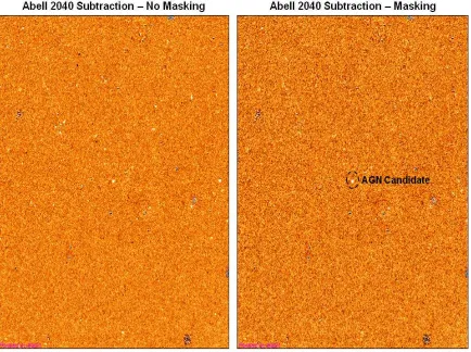
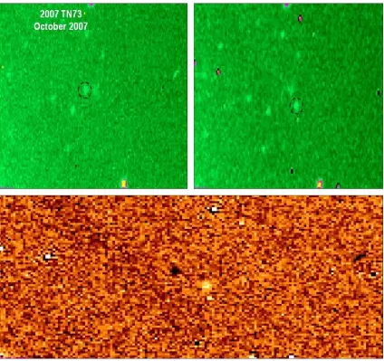
(17) Figure 9.3.2.1. Image and reference from the 2.5-m INT at ING, La Palma (Irwin & Irwin, 2003).. Figure 9.3.2.2. Subtraction by Miller using IDL computer algorithms.. Figure 9.3.2.3. Subtractions by Astier and Irwin (Irwin & Irwin, 2003).. Figure 9.3.2.4. Subtractions by Bond and Irwin (Irwin & Irwin, 2003).. Figure 9.3.3.1. Image and reference from the 3.6-m CFHT on Mauna Kea (Astier 2005).. Figure 9.3.3.2. Comparison of the Astier and Miller subtractions both using the OIS method.. Figure 9.4.1.1. Image and reference of Abell 1006 from the 0.4-m ARI SchmidtCassegrain (Holmes, 2006).. Figure 9.4.1.2. 1st degree space-varying subtraction Figure 9.4.1.1 with the DFB.. Figure 9.4.1.3. Close-up of anonymous galaxy in Abell 1066 and the OIS.. Figure 9.4.2.1. Image and reference of Abell 1831 from the 0.4-m ARI SchmidtCassegrain (Holmes, 2006).. Figure 9.4.2.2. 1st degree space-varying subtraction Figure 9.4.1.1 with the DFB.. Figure 9.4.2.3. Close-up of anonymous galaxy in Abell 1831 and the OIS.. Figure 9.4.3.1. Image and reference of SN 1999av from the Danish 1.54-m and CTIO 1.5-m telescopes, respectively.. Figure 9.4.3.2. First successful OIS of the image and reference in Figure 9.4.3.1.. Figure 9.5.1.1. Image and reference from the NOAO DLS (Pennypacker, 2004).. Figure 9.5.1.2. Random background mask used to cover bad pixels in the image and reference.. Figure 9.5.1.3. OIS subtraction using a constant kernel.. Figure 9.5.2.1. OIS of Figure 9.4.1.1 using a 1st degree kernel and DBF.. Figure 9.5.2.2. Close-up of NGC 3326 and the OIS revealing residual light from the AGN candidate.. 17.

(18) Figure 9.5.3.1. OIS of Abell 2040 using images from the ARI 0.4-m telescope.. Figure 9.6.2.1.1. Image and reference from the DLS (Pennypacker, 2004-2007).. Figure 9.6.2.1.2. Moving object signatures of three asteroids in the field of view.. Figure 9.6.2.1.3. Close-ups of an image, reference, and OIS from the DLS.. Figure 9.6.2.2.1. Image and reference of 2007 TN73 from the ARI 0.81-m telescope (Holmes, 2006-2007).. Figure 9.6.3.1.1. Image and reference of 1999 YF3 from the ARI 0.61-m prime focus telescope (Holmes, 2006-2007).. Figure 9.6.3.1.2. OIS of the image and reference shown in Figure 9.6.3.1.1.. Figure 9.6.3.1.3. Orbit of 1999 YF3 (JPL Small-Body Database Browser).. Figure 9.6.3.2.1. Image of a crowded star field taken from LONEOS at the Lowell Obervatory (Koehn, 2005).. Figure 9.6.3.2.2. OIS of the crowded star field shown in Figure 9.6.3.2.1.. Figure 9.6.3.2.3. Close-up of the crowded star field image in Figure 9.6.3.2.1.. Figure 9.6.3.2.4. OIS of the crowded star field image in Figure 9.6.3.3.. Figure 9.6.3.2.5. Close-up of the NEO from Figures 9.6.3.2.3 and 9.6.3.2.4.. Figure 9.6.3.2.6. Three NEOs detected in the full subtraction of Figure 9.6.3.2.1.. Figure 9.6.4.1.1. Image of Varuna and an unidentified KBO from the 2.5-m INT (Ruiz-Lapuent, 2007).. Figure 9.6.4.1.2. Orbit of Varuna (JPL Small-Body Database Browser).. Figure 9.6.4.2.1. Image and reference of Eris taken from the 2.5-m INT, La Palma (Ortiz, 2006-2007).. Figure 9.6.4.2.2. OIS of the image and reference in Figure 9.6.4.2.1.. Figure 9.6.4.2.3. Close-up of Eris on the image, reference, and OIS.. Figure 9.6.4.3.1. Image and reference of P/2006 U5 from the ARI 0.81-m telescope (Holmes, 2006-2007).. 18.

(19) Figure 9.6.4.3.2. OIS of P/2006 U5 using the image and reference in Figure 9.6.4.3.1.. Figure 9.6.4.3.3. Orbit of P/2006 U5 (JPL Small-Body Database Browser).. Figure 9.6.5.1.1. Three CTIO images from 2002 that make up the field of view of the SN 1987A (Rest, 2006).. Figure 9.6.5.1.2. OIS of the images shown in Figure 9.6.5.1.1.. Figure 9.6.5.1.3. Close-up of the newly-discovered 3rd ring within the SN 1987A light echoes.. Figure 9.6.5.1.4. Close-up of the 1st and 2nd rings within the SN 1987A light echoes.. Figure 9.6.5.2.1. GSC03549-02811, the parent star of TrES-2 (Mandushev, 2007).. Figure 9.6.5.2.2. Time-varying object observed in the TrES-2 data.. Figure 10.1.1. Image and reference of the galaxy cluster Abell 1656a from the ARI 0.41-m Schmidt Cassegrain telescope.. Figure 10.2.1. Stamp of a spherically-shaped galaxy in the cluster Abell 1656a used to test the quality index Q.I.. Figure 10.2.2. Constant kernel subtractions of the spherical galaxy in Abell 1656a using both the DFB and GCB.. Figure 10.2.3. 1st degree space-varying kernel subtraction of the spherical galaxy in Abell 1656a using both the DFB and GCB.. Figure 10.2.4. Quality Index vs. Degree of the space-varying kernel and the type of basis, DFB and GCB.. Figure 10.3.1. Stamp of an elliptically-shaped galaxy in the cluster Abell 1656a used to test the quality index Q.I.. Figure 10.3.2. Constant kernel subtractions of the elliptical galaxy in Abell 1656a using both the DFB and GCB.. Figure 10.3.3. 1st degree space-varying kernel subtraction of the elliptical galaxy in Abell 1656a using both the DFB and GCB.. Figure 10.3.4. Quality Index vs. Degree of the space-varying kernel and the type of basis, DFB and GCB.. 19.

(20) Figure A6.1.1. The pixels around the kth stamp that are included in the calculation of  k l ,m .. Figure A7.2.1. Location of matching centroids from the two images.. Figure A7.2.2. Position vectors of the two matching centroids.. Figure A7.2.3. Displacement vector of the first centroid.. Figure A7.2.4. Addition of the displacement vector of the first centroid to the second.. Figure A7.2.5. Definition of the rotation angle Θ.. Figure A7.2.6. Calculation of the rotation angle Θ.. 20.

(21) Chapter 1 1.1. Introduction. Statement of the Problem. Objects that vary in brightness or in position over time are of prime importance in modern astronomy and astrophysics. There are many such objects including:       . Active galactic nuclei (AGN) and quasi-stellar objects (QSOs) that vary in brightness when the black hole cores of galaxies or their surrounding accretion disks change brightness over time, Variable stars such as a Cepheid variable that changes brightness when it expands and contracts in size or a cataclysmic variable that fluctuates in brightness with a hot spot on an accretion disk orbiting a white dwarf companion, Supernovae (SNe) exploding in distant galaxies that can become nearly as bright as their host galaxies, Microlensing events that produce a sudden change in brightness as light from a background source bends through the gravitational field of a foreground source along the line-of-sight, Gamma ray bursts (GRBs) linked to hypernovae lasting on average 30-seconds and generating a hundred times the energy of an ordinary SNe, Extrasolar planets transiting their parent stars slightly dimming the stars, Moving objects across a field of view such as asteroids, comets, Kuiper Belt objects (KBOs) and even SNe light echoes.. Searches for these objects are undertaken by acquiring an image of the region of the sky followed by a second image taken at a later time. The length of the time interval is dependent upon what type of object is being sought. For example, for AGN and SNe the typical time interval is 30 or more days. For SNe light echoes the time is on the order of years while for asteroids and KBOs it is on the order of hours. Ideally, both images are taken with the same telescope using the same filter and chargecoupled device (CCD). The two images are carefully aligned and subtracted pixel-bypixel with the subtracted image revealing any changes in light, called residual light, during the time period between the two images. Astronomical CCD images represent nearly ideal computational and mathematical data. CCDs exhibit a linear response. They organize their output images in a tractable rectangular stable matrix, with uniformity that provides predictability from image to image. Many subtraction methods use a convolution procedure (Phillips & Davis 1995; Tomaney & Crotts 1996; and Irwin & Irwin 2003). Identifying the two images as I and R (i.e., the image and reference, respectively), a convolution kernel K is constructed. The R image, typically the better-seeing of the two, is convolved to match the worse-seeing image I. The convolution R  K is determined, and a pixel-by-pixel subtraction S is. 21.

(22) given by S  I  R  K  . For a kernel K of size L x L, where L is odd, the convolution is defined as:. R  K i, j. . i  w. j  w.  R. u i  w v  j  w. u ,v. K u i  w1,v  j  w1. (1) 1 L  1 and (i,j) represents the ij-th pixel of the convolution. 2 R  K is a match to I, but not equal to I since R and I contain a time-varying or positionchanging object. The subtraction S  I  R  K  reveals only the residual light from that object. All of the other light sources subtract into the background, with the exception of sources with saturation or blooming and hot pixels due to cosmic rays.. where w . 1.2. History of Image Subtractions. The current development of subtraction methods is the result of searches for microlensing events caused when an object in the foreground passes along the line of sight of a star in the background. In particular, the microlensing caused by massive compact halo objects in the MACHO Project was the source of the “optimal image subtraction” (OIS) method used in this study. The MACHO Project was a collaboration of the Mt. Stromlo Observatory, Siding Spring Observatory, the Center for Particle Astrophysics at the University of California (Santa Barbara, San Diego, and Berkeley) and the Lawrence Livermore National Laboratory. The project tested the hypothesis that a significant fraction of the dark matter in the halo of the Galaxy consists of objects like brown dwarfs or planets [i.e., machos, see MACHO Project (1997)]. Because of the low probability of having the ideal alignment necessary to produce a microlensing event, images had to be taken of crowded star fields. This led to event searches among hundreds of thousands, if not, millions of stars in the effort to identify the few events that would be expected within such a sample. Therefore, to conduct these searches successfully, subtraction methods were needed that were both effective and computationally efficient. The first subtraction method was done utilizing catalogs of objects within the image of a crowded star field, constructed using the software DoPHOT or its derivatives. The pointspread functions (PSFs) of the objects on the image were measured then compared to preset PSF analytical models. The types of objects being sought such as stars, double stars, and various-shaped galaxies had their own analytical models, each with a defining set of independent parameters. Non-linear regression methods were used to obtain the best fit of a catalog object PSF to these parameters. Given a match with a pre-set model, the object in the catalog was classified (Schecter, et al., 1993; Alard, 2000).. 22.

(23) Of the identified objects in the catalog, the corresponding best-fit analytical model was used to subtract the objects from the image, leaving behind only those objects with PSFs that had no best fits (i.e., objects with residual light). This method has proven successful in the identification of microlensing events, and is still in use (Alard, 2000). In the microlensing searches, the first use of a convolution appeared in 1996 (Tomaney & Crotts, 1996) using an algorithm developed by Phillps & Davis (1995). In their 1996 paper, Tomaney & Crotts used a sub-image 128 x 128 pixels in size to test the algorithm. A non-variable star was identified near the center of the sub-image, and an elliptical Gaussian kernel was derived as the best fit of the full-width half maximum (FWHM) of the image. That is, the star in the better-seeing reference R was degraded to match the PSF of that same star in the worse-seeing image I. The R sub-image was convolved with the best-fit kernel then subtracted pixel-by-pixel from the I sub-image. In the testing of this method, Tomaney & Crotts made an interesting discovery. They best-fit kernel used in the sub-image subtraction did not necessarily perform well elsewhere in the main image, in some cases as few as 500 pixels away from the subimage. This suggested the need for a space-varying kernel. In turn, this led to the partitioning of the image and reference into 128 x 128 pixel subimages, selecting a non-variable star in each sub-image, deriving the best-fit elliptical Gaussian kernel for each, subtracting with the convolution of that kernel, and merging the subtracted sub-images back into a single subtraction (Alard, 2000). Using a constant, elliptical Gaussian kernel but updating that kernel every 128 pixels is one method of approximating a space-varying kernel. From this approach spawned the development of the “optimal image subtraction” method proposed by Alard & Lupton (1998).. 1.3. Optimal Image Subtraction Method (OIS). The OIS method constructs a convolution kernel K using a set of ~150 non-variable stars [hereinafter called “stamps” after Alard (1998)], found on the two images to be subtracted. These stamps are typically 20 x 20 pixels in size. They correspond from the image to the reference, and are randomly distributed (i.e., a representative sample over both). Given a set of basis vectors {K n : n  1,2,..., N } defined in Chapter 3, the set of stamps is N. used to build a kernel K   a n K n . The following equation is defined over the stamps: n 1.  N  N I  R  K   R    a n K n    a n R  K n   n1  n 1. 23.

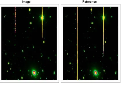
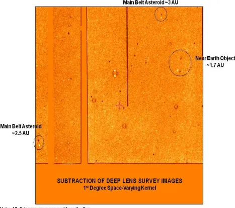
(24) which is then solved in the least square sense for {a n : n  1,2,..., N } , the coefficients used in the basis vector expansion for K. The subtraction is a pixel-by-pixel calculation given by S  I  R  K  . This approach can be used to construct a single space-varying kernel eliminating the need to partition the image and reference into 128 x 128 pixel sub-images and calculating as many as 256 constant, elliptical-Gaussian kernels.. 1.4. Demonstration of the OIS Method. Consider two CCD images taken of the same area of the sky with the same telescope and same filter but at different times. Once aligned (i.e., the images are aligned pixel-bypixel to sub-pixel accuracy), there remain differences due to varying seeing atmosphericgenerated conditions between the two images and varying conditions within the system optics. In effect, it is not possible to acquire a pair of identical images. Figure 1.4.1 shows two aligned images from the Deep Lens Survey (National Optical Astronomy Observatory). These were taken with the 4-m Victor M. Blanco telescope located at the Cerro Tololo Inter-American Observatory, Chile. The same filter was used in both but the images are separated in time by one year. The brightness-varying objects being sought were AGN and SNe. (Pennypacker, 2004-2007).. 24.

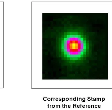
(25) Figure 1.4.1. Image and reference from the CTIO 4-m Blanco telescope, Chile (Pennypacker, 2004-2007). Figure 1.4.2 shows matching stamps from the image and the reference. Clearly, the image is the worse-seeing of the two. There is more background in the image and the FWHM of the star within that stamp is larger.. 25.

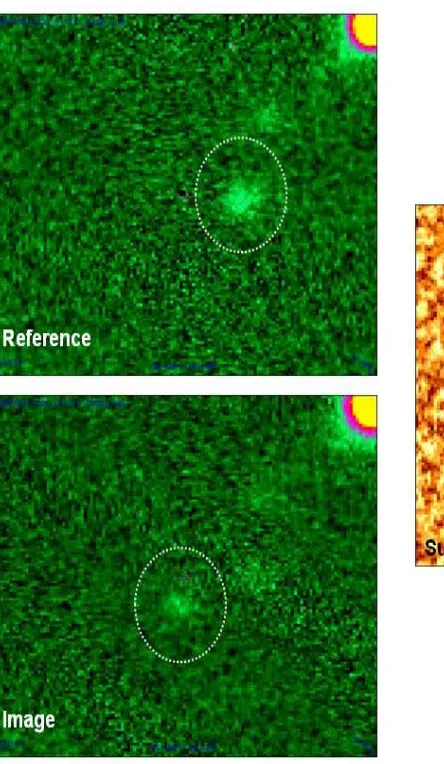
(26) Figure 1.4.2. Corresponding stars in stamps from the image and reference in Figure 1.4.1. Another way to detect the difference between the image and reference is to look at the profile or point-spread function (PSF) as shown in Figure 1.4.3. The differences in intensity counts (flux) and FWHM can be seen.. 26.

(27) Figure 1.4.3. Point-spread functions of the stars in the two stamps in Figure 1.4.2. In order to subtract these two stamps, it is necessary to first adjust the star in the stamp from the reference to match the corresponding star within the image (i.e., match the better-seeing stamp with the worse-seeing stamp). This process is done mathematically using a convolution. A constant convolution kernel K is derived using the OIS of Alard (2000). It is applied to the better-seeing image to match the two stars (i.e., the image with a PSF that has the smaller FWHM). The kernel is a small matrix typically 13 x 13 that is applied across the better-seeing image. It is centered on each pixel and replaces that pixel with a weightedaverage of the surrounding pixels, based upon the width of the kernel and using the kernel values as the weights. See Equation (1) in Chapter 1.1. This has the effect of spreading out the smaller PSF of the better-seeing image to match it with the larger, worse-seeing PSF. See Figure 1.4.4, and note that the star from the convolved reference stamp has a PSF which more nearly matches the star from the image stamp. With a matched PSF, the subtraction is done pixel-by-pixel S  I  R  K  . Figure 1.4.6 is the subtraction of the two stamps showing only random background. This implies, to the sensitivity of the image and reference, that there was no change in this star during the one-year interval of time. 27.

(28) Figure 1.4.4. Point-spread functions of the image stamp and convolved reference stamp. The reference was convolved using the OIS method with a constant convolution kernel K. The PSFs are better matched after the convolution.. 28.

(29) Figure 1.4.5. Stamps from the image and the convolved reference.. 29.

(30) Figure 1.4.6. OIS of the two stamps in Figure 1.4.5. The star in the stamps subtracts out to random background, revealing there were no changes in this star from the image to the reference. By way of comparison, a sub-image containing a galaxy with an AGN candidate was selected from the same image and convolved reference. See Figure 1.4.7 for the profiles or PSFs of the two. The PSFs are decidedly different so the subtraction does not show random background as does the subtraction of the star. Instead it shows residual light from the active nucleus. See Figure 1.4.8.. 30.

(31) Figure 1.4.7. Sub-images and PSFs of a galaxy with a suspected AGN. The first sub-image comes from the image and the second from the convolved reference. The PSFs are not matched, indicating residual light between the two (i.e., a change in the galaxy from the image to the reference).. 31.

(32) Figure 1.4.8. OIS of the two sub-images containing the galaxy with a suspected AGN. Residual light is shown revealing the presence of the AGN.. 32.

(33) Chapter 2 2.1. The Convolution Kernel. Introduction. As indicated before, let I and R be two aligned images taken of the same area of the sky using the same telescope and CCD with the same filter, but at different times. I is the worse-seeing image to be matched and R is the better-seeing image, called the reference. R is used to match I using a convolution kernel K. In the first derivation, it is assumed that the kernel K is constant. That is, the PSF of the stamps is not varying over the image in such a way that the kernel will change its size or any of its entry values. If there are variations in the PSF over the image, a space-varying kernel can be used. The derivation of a space-varying kernel of fixed size follows in Chapter 2.3, again using the OIS methods of Alard (2000). To derive the kernel, first be certain I and R are carefully aligned to the sub-pixel level. Second, select a set of stamps containing corresponding stars selected from I and R. These stamps are typically 21 x 21 sub-images, and must be uniformly distributed over I and R. They are used to set up the equation I  R  K to be solved in the least squares sense for the convolution kernel K. With the kernel K in hand, it is applied to R as a convolution (i.e., R  K ) with this result subtracted from I. This gives the pixel-by-pixel subtraction S  I  R  K , which is then analyzed for brightness-varying or position-changing objects.. 2.2. Constant Kernel. Let I and R be the aligned image and reference, and of size SR x SC. Identify the following sets of stamps {I k : k  1,2,..., P} within the image I, and let {Rk : k  1,2,..., P} be the corresponding stamps within the reference R. P represents the number of stamps to be used in the derivation of the convolution kernel K. Each stamp is ηk x ηk where ηk is assumed to be odd. The process of identifying the set of stamps is described in Chapter 4.2. The selection and processing of these stamps is one of the main undertakings of this work. Let K be an L x L kernel, where L is odd, to be applied to R in a convolution match with I. Define the basis vectors for the kernel K, {K n : n  1,2,..., N } where N is fixed and N. 1  N  L2 . Expanded with respect to this basis, the kernel is given by K   a n K n . n 1. A discussion of different choices for the basis vectors is given in Chapter 3. For this derivation it assumed that the basis is already specified. Therefore, the mathematical task is to solve for {a n : n  1,2,..., N } , the coefficients of the basis expansion.. 33.

(34) Consider the equation I  R  K to be solved in the least squares sense over the stamps. Let Ek,i,j be defined as the following: N N   E k , i , j  ( R k  K ) i , j  ( I k ) i , j   Rk   a n K n   ( I k ) i , j   a n ( Rk  K n ) i , j  ( I k ) i , j n 1 n 1   i, j. Where 1  k  P , 1  i  nk , and 1  j  nk . Ek,i,j represents the error between the ij-th pixels of I and the k-th convolved stamp. The sum of the squares of the errors over all pixels and stamps gives the least squares function from which the linear system is obtained that determines the values of {a n : n  1,2,..., N } : k. k. k. k.  N  F (a1 , a 2 ,..., a N )   ( E k ,i. j )     a n ( Rk  K n ) i , j  ( I k ) i , j  k 1 i 1 j 1 k 1 i 1 j 1  n 1  P. P. 2. 2. The multi-variable least squares solution is given by: F  0. F   al al.  P k  k  P k k    ( E k ,i. j ) 2    2 E k ,i. j E k ,i , j  0   al  k 1 i 1 j 1  k 1 i 1 j 1. where l  1,2,..., N . This produces the following:    N  E k ,i , j    a n ( R k  K n ) i , j  ( I k ) i , j   ( Rk  K l ) i , j al al  n 1  k. k. k. k.  N    a n ( R k  K n ) i , j  ( I k ) i , j ( R k  K l ) i , j  0  k 1 i 1 j 1  n 1  P. P  k k  N  a ( R  K ) ( R  K )  ( I k ) i , j ( Rk  K l ) i , j     n k n i, j   l i, j k 1 i 1 j 1  n 1 k 1 i 1 j 1 P.  P k  k  P  k k  a n   ( Rk  K n ) i , j ( Rk  K l ) i , j    ( I k ) i , j ( Rk  K l ) i , j  n 1  k 1 i 1 j 1  k 1 i 1 j 1 N. where l  1,2,..., N . 34.

(35) Finally, the following N x N linear system is set up: Ma=b P. k. k. P. k. k. where M n ,l   ( Rk  K n ) i , j ( Rk  K l ) i , j and bl   ( I k ) i , j ( Rk  K l ) i , j k 1 i 1 j 1. k 1 i 1 j 1. n  1,2,..., N and l  1,2,..., N .. This linear system is solved for the vector a . a, 1. a 2 , , a N. . T. , which contains the. N. coefficients needed to express the convolution kernel K   a n K n as an expansion of the n 1. basis vectors. In this study, LU decomposition with single-precision arithmetic was used to extract this solution. However, this approach does not take advantage of the fact this system is positive definite, which allows for the use of more efficient system solvers (Astier, 2004).. 2.3. Space-Varying Kernel. To allow for the possibility that the kernel K varies across the image, the coefficients an of the expansion are re-defined as an(x,y) where (x,y) are pixel coordinates of the aligned images I and R. As proposed by Alard (2000) it is assumed that these coefficients are bivariate polynomials of (x,y), with each an(x,y) multiplying one basis vector Kn: d d m. a n ( x , y )     n , m ,l x m y l m0 l 0. N. K ( x, y )   a n ( x, y ) K n n 1. The degree of the polynomial is d. an(x,y) contains a total of. 1 (d  1)(d  2) terms. 2. Functions other than a polynomial in (x,y) could be used. In general, a set of basis functions can be defined  m ,l ( x, y ) : 0  m  D1 , 0  l  D2 where the coefficients of. . . D1 D2. the kernel basis vectors become  n ( x, y )    n,m ,l  m,l ( x, y ) . In the Alard (2000) m0 l 0. approach,  m,l ( x, y )  x m y l for 0  m  d , 0  l  d  m , and in the constant kernel solution  m ,l ( x, y )  1 for all m, l, and (x,y). In this study no other functional forms for.  m,l ( x, y ) have been investigated, other than the bi-variate polynomials proposed by Alard (2000); however, this would make for an interesting future study.. 35.

(36) Consider the equation I  R  K to be solved in the least squares sense over the set of stamps. As before with the constant kernel solution, let Ek,i,j be defined as the following: N. N. n 1. n 1. E k ,i , j  ( Rk  K ) i , j  ( I k ) i , j  R k   a n ( K n ) i , j  ( I k ) i , j   a n ( Rk  K n ) i , j  ( I k ) i , j. where 1  k  P , 1  i   k , and 1  j   k . On an individual stamp, the bi-variate polynomial an(x,y) is assumed to be constant, and set to its value at the coordinates of the center pixel ( xˆ k , yˆ k ) . This constant approach over a stamp is proposed by Alard (2000). It may be possible to weaken this condition by allowing an(x,y) to vary across the stamp but this has not been studied: N. N. Ek ,i , j  ( Rk  K )i , j  ( I k )i , j  Rk   an ( xˆk , yˆ k )( K n )i , j  ( I k )i , j   an ( xˆk , yˆ k )( Rk  K n )i , j  ( I k )i , j n 1. n 1.  m l  E k ,i , j   a n ( xˆ k , yˆ k )( Rk  K n ) i , j  ( I k ) i , j       n ,m ,l xˆ k yˆ k ( Rk  K n ) i , j  ( I k ) i , j n 1 n 1  m  0 l  0  N d d m   m l E k ,i , j       n ,m ,l xˆ k yˆ k ( Rk  K n ) i , j   ( I k ) i , j n 1  m  0 l  0  N. N. d d m. The sum of the squares of the errors over all pixels and stamps gives the least squares function from which the linear system is obtained that determines the α-coefficients that define each of the bi-variate polynomial functions an(x,y):.  N  d d m   m l F   ( E k ,i. j )        n,m ,l xˆ k yˆ k ( Rk  K n ) i , j   ( I k ) i , j  k 1 i 1 j 1 k 1 i 1 j 1  n 1  m  0 l  0   P. k. k. P. 2. k. k. 2. The least squares solution is given by:. F  0 F    q , r , s  q , r , s.  P k k  P k k     ( E k ,i. j ) 2     2 E k ,i. j E k ,i , j  0    q , r , s  k 1 i 1 j 1  k 1 i 1 j 1. where q  1,2,..., N and for each value of q, r  0,1,..., d , s  0,1,..., d  r . This gives the following:. 36.

(37)     N  d d m  m l r s E k ,i , j       n, m,l xˆ k yˆ k ( Rk  K n ) i , j   ( I k ) i , j   xˆ k yˆ k ( Rk  K q ) i , j a q ,r , s  q ,r , s  n 1  m0 l 0  .  N  d d m  r s  m l ˆ ˆ ˆ ˆ  x y ( R  K )  ( I )        n , m ,l k k k n i, j k i , j  x k y k ( Rk  K q ) i , j  0 k 1 i 1 j 1  n 1  m  0 l  0   P. k. k. P k k. N. d d m. n,m,l xˆk. mr. k 1 i 1 j 1 n1 m0 l 0 N. P k  k. d d m.   n1 k 1 i 1 j 1 m0 l 0. N. d d m P. nk. n,m,l. xˆ k. nk. n,m,l xˆk. P k k. l s r s yˆ k (Rk  Kn )i, j (Rk  Kq )i, j  xˆk yˆ k (I k )i, j (Rk  Kq )i, j k 1 i 1 j 1. m r. mr. n1 m0 l 0 k 1 i 1 j 1. yˆ k. l s. P k  k. r s (Rk  K n ) i, j (Rk  K q ) i, j   xˆ k yˆ k (I k ) i, j (Rk  K q ) i, j k 1 i 1 j 1. nk. P. nk. l s r s yˆ k (Rk  K n )i, j (Rk  Kq )i, j   xˆk yˆ k (I k )i, j (Rk  Kq )i, j k 1 i 1 j 1. A re-organization of the above equation produces the linear system:.  P k k m  r l  s  P k k r s  n,m,l  xˆ k yˆ k (Rk  K n ) i, j (Rk  K q ) i, j    xˆ k yˆ k (I k ) i, j (Rk  K q ) i, j  n1 m0 l 0  k 1 i 1 j 1  k 1 i 1 j 1 N. d d m. where q  1,2,..., N and for each q, r  0,1,..., d , s  0,1,..., d  r . In other words, for each q  1,2,..., N there are Q x Q linear system where Q . 1 (d  1)(d  2) equations. This defines a 2. 1 N (d  1)(d  2) . For an example of this linear system, 2. refer to the Appendix A2.3.. 2.4. Conclusions. In this chapter, the system of equations for the OIS convolution kernel K was derived for the constant kernel case and the space-varying case with a fixed-size kernel. The three important equations presented or developed thus far are: (1). Definition of a Convolution. R  K i, j. 37. . i  w. j  w.  R. u i  w v  j  w. u ,v. K u i  w1,v  j  w1.

(38) where w  (2). 1 L  1 and (i,j) represents the ij-th pixel of the convolution. 2. Linear System for the Constant OIS Kernel P. k. k. M a = b where M n,l     ( Rk  K l ) i , j ( R k  K n ) i , j and k 1 i 1 j 1. P. k. k. bl   ( I k ) i , j ( Rk  K l ) i , j n  1,2,..., N and l  1,2,..., N . k 1 i 1 j 1. The solution is the vector a  (3).  a, 1. a2 ,  a N. . T. .. Linear System for the Space-Varying, Fixed-Size OIS Kernel.  P k k m  r l  s  P k k r s  n,m,l  xˆ k yˆ k (Rk  K n ) i, j (Rk  K q ) i, j    xˆ k yˆ k (I k ) i, j (Rk  K q ) i, j  n1 m0 l 0  k 1 i 1 j 1  k 1 i 1 j 1 N. d d m. where q  1,2,..., N and for each q, r  0,1,..., d , s  0,1,..., d  r .. . The solution is the vector    n, m,l. . T. where n  1,2,..., N , m  0,1,..., d , and. l  0,1,..., d  m . N. N. The kernel K   a n K n in the constant case and K ( x, y )   a n ( x, y ) K n in the spacen 1. n 1. d d m. varying case where a n ( x, y )     n, m ,l x m y l . With the kernel in hand, Equation (1) is m0 l 0. used to calculate the convolution of the reference R  K followed by the subtraction S  I RK .. 38.

(39) Chapter 3 3.1. Basis Vectors. Introduction. Alard (1999, 2000) proposed what are called the “Gaussian components basis” (GCB), although the precise mathematical nature of this basis was not fully specified. A clearer explanation and definition is provided by Astier (2004-2007). Essentially, the GCB utilizes the Gaussian structure of the point spread functions (PSFs) of the stars within the stamps, and produces a kernel with Gaussian structure that is symmetric off its center then trails to zero toward its edges. A detailed definition of the GCB is provided in Chapter 3.3. However, it is important first to understand that the GCB produces a subspace of the vector space of L x L kernels K (typically, L = 13). That is, any kernel generated by the GCB possesses the Gaussian structure off of its center. If kernels are needed that do not have this centered-structure, the GCB is unable to produce them. To illustrate this point, the typical-sized kernel is 13 x 13, which means the space of all kernels has a dimension of 132 = 169. If Nc is the number of Gaussian components and {d k : k  1,2,..., N c } is the set of degrees of these components, the total number of vectors Nc 1 is N  1   (d k  1)(d k  2) . Following Alard (2000) and Astier (2004-2007), Nc = 3 k 1 2 and d1 = 6, d2 = 4, and d1 = 2 giving N = 50 < 169, so the span of the GCB does not equal the space of all kernels.. The delta function basis (DFB) is introduced as an alternative to the GCB. This basis has the same number of vectors as the dimension of the space of all kernels. For a 13 x 13 kernel, this means the DFB contains 132 = 169 vectors. Each vector contains all zeros with the value of 1 in only one of the entries, with the location of that 1 varying across the 169 entries to produce a total of 169 vectors. The advantage of the DBF over the GDB is that if a kernel is needed that is not symmetric off of its center, the DBF will produce it since the span of the DBF equals the space of all the kernels. The GCB cannot, since such kernels lie outside of the span of the GCB. The disadvantage of the more flexible DFB is that it is computationally expensive. With even a 1st degree space-varying kernel on a 1K x 1K image and reference, the total number of arithmetic calculations is ~470 million. The computation time is about an hour on a Hewlett-Packard Pavilion zd8000 laptop with an Intel Pentium 4 processor and 2.80 GHz processing speed. This compares to about 20 minutes for the GCB. See Table 3.1.. 39.

(40) Table 3.1.. Estimated Computation Time.. Image & Reference Size: Kernel Size: Size of DFB: Size of GCB: Processing Speed:. Degree of Kernel 0 1 2. Linear System Size DFB GCB 169 50 507 150 1014 300. 1K x 1K 13 x 13 169 vectors 50 vectors 2 mips. # of Calculations (x 106) DFB GCB 5 0.1 130 3 1043 27. # of Kernel Calculations (x 106) 337 341 350. Computation Time (minutes)1 DFB GCB 5 5 60 20 180 60. 1. These times are determined empirically and include both the time to compute the solution to the linear system and the convolution.. Despite this disadvantage of computational speed, the DBF performs better than the GCB in producing optimal image subtractions. For a demonstration of this fact, see Chapter 9, Validation of the IDL Computer Codes, and Chapter 10, Subtraction Quality.. 3.2. Delta Function Basis. The basis vectors for the L x L kernel K are defined as {K n : n  1,2,..., N } , where L is odd and 1  N  L2 . Two different bases were considered, the delta function basis (DFB) and Gaussian components basis (GCB). The DFB was defined for the full L2 dimension of the kernel. A basis vector is an L x L matrix with 0’s in all entries except in one entry there is 1. The 1 varies across all of the L2 entries to produce the basis. The formal definition of the DFB is. K n i, j.   n , L (i 1) j where n  1,2,..., L2 while. 0 if a  b i  1,2,..., L , and j  1,2,..., L for each value of n.  a ,b   is the Kronecker 1 if a  b delta. Since L is odd the centered delta function basis vector is included, allowing for two images with almost-identical stamps.. 3.3. Gaussian Components Basis. The GCB was not defined for the full L2 dimension of the kernel. Instead, it is defined over an N-dimensional subspace as follows (Alard, 2000; Astier, 2004):. 40.

(41) Nc is the number of Gaussian components, and defines the number of degrees {d k : k  1,2,..., N c } and the number of standard deviations { Kernel k : k  1,2,..., N c } of the components.  Kernel is the standard deviation of the kernel (Astier, 2004). 1 (d k  1)(d k  2) matrices (L x L) 2 to the basis vectors. The total number of basis vectors is. Each component contributes a total of. Nc 1 N  1   (d k  1)(d k  2) k 1 2. 1 ( L  1) then for n  1,2,...N  1 , where each combination of u and v 2 produces one basis vector while 0  u  d k and 0  v  d k  u :. Let Ctr . K n i , j.  (i  Ctr ) u ( j  Ctr ) v e. . ( i  Ctr ) 2  ( j  Ctr ) 2 2 Kernel 2 k 2. 1  i  L and 1  j  L. and ( K N ) i , j. 0 if i  Ctr  j  Ctr  1 if i  Ctr  j  Ctr. The purpose of including KN is to allow for images that are almost identical. This is the centered delta function basis vector that just returns the pixel value (i.e., no weighted average) during the convolution R (i.e., R  K N  R ). The index n  1,2,...N  1 of the basis vectors can be calculated by making use of the following algorithm: Start  1 For k  1,2,...N c 1  k  Start  d k u  v  u (u  3) 2 1 Start  Start  (d k  1)(d k  2) 2 End For. 41.

(42) Nc. where N  1   k . There is a  k block of basis vectors set aside for each of the k 1. components. As per Astier (2004-2007) the following Gaussian components were selected: Nc  3. d  6 , 4 , 2. .    0 .7 , 1 .5 , 2 .0. . Astier established these components empirically, and these values are similar to those proposed by Alard (2000). More recently in an effort to eliminate empirical estimates, Israel, et al. (2007) developed a procedure for selecting optimal components for image sets with different S/N ratios and sampling.. 3.4. Visualization of the Kernel & Gaussian Components. For a visualization of a kernel derived with the GCB, refer to Figure 3.4.1. This shows the optimal constant kernel derived for the two images from the Deep Lens Survey (National Optical Astronomy Observatory) shown in Figure 1.3.1. The 13 x 13 kernel was derived using the three Astier (2004) components and the centered delta function basis vector. The kernel is shown along with a surface rendition and the horizontal and vertical cross sections.. 42.

(43) Figure 3.4.1. OIS constant kernel for the image and reference in Figure 1.4.1. The three Astier (2004-2007) Gaussian components were used for the basis vectors. The kernel consists of the sum of three Gaussian components of 6th, 4th, 2nd degree, and the centered delta function basis vector. The basis contains 50 vectors; 28 make up the 6th degree component, 15 the 4th degree component, 6 the 2nd degree component, and 1 the centered delta function basis vector.. 43.

(44) Figure 3.4.2. 6th degree Gaussian component for OIS constant kernel in Figure 3.4.1.. 44.

(45) Figure 3.4.3. 4th degree Gaussian component for the OIS constant kernel in Figure 3.4.1.. 45.

(46) Figure 3.4.4. 2nd Degree Gaussian component for the OIS constant kernel in Figure 3.4.1.. 46.

(47) Figure 3.4.5. Centered delta function basis vector for the OIS constant kernel in Figure 3.4.1. In comparison, the following is the optimal constant kernel derived for the two images from the Deep Lens Survey using the delta function basis. A total of 169 basis function vectors were used to produce this 13 x 13 kernel.. 47.

(48) Figure 3.4.6. OIS constant kernel for the image and reference in Figure 1.4.1. The delta function basis was used. For algebraic examples of the delta function basis and the Gaussian components basis, refer to the Appendix A3.4. Understanding the nature of these bases is important to the understanding of the overall least squares algorithm used to calculate the convolution kernel.. 48.

(49) Chapter 4 4.1. Selection of the Stamps. Introduction. Prior to any selection of the stamps for use in the least squares algorithm to calculate the convolution kernel, bad pixels in both images, I and R, must be identified and masked. An image identifying the bad pixels in either I or R must be created, and used to mask I and R during the stamp selection procedure. If not, these bad pixels can contaminate the stamps making them outliers, which adversely affect the least squares calculation of the kernel. Among the possible bad pixels are those that are saturated, bloomed, or unused. Saturated pixels occur when the electron count exceeds the range of the silicon chip detector. It is an over-exposure of the detector. Often times, neighboring pixels experience blooming (i.e., linear streaks with increased counts but within the detector range). Unused pixels occur when images are merged together into larger images or are aligned. These pixels contain no data.. 4.2. Identifying & Masking Bad Pixels. The algorithm to process bad pixels used in this study is given in the following: 1) 2) 3) 4). Identify bad pixels in I and R, separately. Flag pixels from I and R that are bad in either I or R. Determine the background sky, mean µ and standard deviation σ for both I and R. Replace the flagged pixels with random values of background sky within 1-σ of µ in both I and R.. The resulting masking of I and R forms “ghost” images, IS and RS. It is from IS and RS that the stamps are selected, and not from I and R. Automated procedures for constructing IS and RS were written using IDL and combined with utilities from the IDL Astronomy User’s Library maintained by the NASA Goddard Space Flight Center [GSFC; Greenbelt, MD - see Landsman (2004)]. The background sky mean µ and standard deviation σ are determined for both I and R. The following images are constructed: IQ . I  I. I. RQ . R  R. R. At each pixel in IQ and RQ the number of standard deviations from mean sky is recorded. The minimum of the median and standard deviation of the pixels in IQ and RQ is calculated:. 49.

(50)  Q  min[median( IQ), median( RQ)]  Q  min[ IQ ,  RQ ] A range of light RMin to RMax is set in which the stamps are selected (i.e., the pixels not within this range are masked to form IS and RS):  max[max(IQ), max(RQ)]   Q FMin  R Min   Q  g Min   Q  FMin  Q.    .  max[max(IQ), max(RQ)]   Q FMax  RMax   Q .    . f Min  max(3, g Min ). f Max   Q  FMax  Q. Finally, the pixels that satisfy the following condition are used in the “ghost” images to find the stamps while the other pixels are masked, including any unused pixels:. f. Min.  .  I  I   Q  f Max I  f Min R  R   Q  f Max R. . The following shows the empirical results in setting the parameters RMin and RMax: . For well-behaved images with no significant amount of saturation or blooming (e.g., no linear streaks), [ R Min , RMax ]  [0.25 , 0.75] seems to work well. Essentially, most of the light is available for the search of stamps. To obtain all of the light [ R Min , RMax ]  [0.00 , 1.00]. . For significant saturation or blooming, especially with linear streaks, or extensive light from the Moon or nebulae, [ R Min , RMax ]  [0.00 , 0.15] seems to work. Essentially, the bright, diffuse light is not available for stamps, and the stamps must be derived from the fainter stars.. Figure 4.2.1 shows an example of identifying the bad pixels and masked to form the “ghost” images for the two images from the Deep Lens Survey (National Optical Astronomy Observatory) shown in Figure 1.4.1. In this instance, there was significant saturation and blooming including linear streaking. The range of light that was kept for the “ghost” images was defined by [ R Min , RMax ]  [0.00 , 0.15] .. 50.

(51) Figure 4.2.1. Original image and the masked “ghost” image. It is from the masked “ghost image” that stamps are selected for the OIS. The purpose of the masking is to identify areas on the image where not to look for stamps (e.g., in a diffuse cloud, unused pixels, saturated areas, areas brightly lit by the Moon). It could be argued that these areas could be set to a fixed value, say 10,000 less than minimum sky. However, the IDL utilities from the NASA Goddard Space Flight Center (notably the tool FIND as described in the Chapter 4.3) have a hard time working on these areas with fixed values, so the replacement with random background circumvents this problem with these utilities.. 4.3. Stamp Selection. The selection of the stamps is very important. It is best that they include single stars with minimal light contamination and be uniformly distributed over I and R. An automated stamp selection code was written as part of this study. Among the many checks that it makes (e.g., single stars, minimal light contamination), it does not check for the uniform distribution. Future versions of the code need to include this check.. 51.

(52) The following IDL utilities from the Goddard Space Flight Center were used (Landsman, 2004). They are applied to the worse-seeing ghost image, IS:  . SKY FIND. SKY calculates the background statistics of IS including the mean and standard deviation. The standard deviation is an input parameter into FIND that identifies the centroids of point sources on IS. Actually a modified version of FIND was written by the author, NEWFIND, which suppresses the print commands and iterations of FIND. Once identified, the centroids are individually examined. A (2σ+1) x (2σ+1) stamp is placed around the centroid where σ is derived from the approximate FWHM of the worse-seeing image , a 2-D Gaussian fit is performed, and the stamp is increased by 2 x 2 with a second 2-D Gaussian fit performed. The size of the stamp is increased by 2 x 2 until the percent difference in 0.1%)..  12   22 is less than a pre-set parameter (typically set at. The estimated kernel sigma is calculated, σKernel by comparing the first two stamps from IS and RS (i.e., the first two stamps not overlapping the edge of the image). A 2-D 1 Gaussian fit is performed on the two stamps and  Kernel   IS ,1   RS ,1   IS , 2   RS ,, 2 2. . . The stamps are re-sized to accommodate the kernel then checked to see if they overlap the boundary of the image, meet the user-defined sharpness and roundness statistical criteria of NEWFIND, have a flux exceeding the user-defined percent of the maximum flux of the stamps, and overlap one another. Stamps that fail any one of these tests are rejected.. 4.4. Rejection of Stamps During Kernel Calculation. Once defined, the stamps are used to calculate the convolution kernel K by solving the equation I  R  K in the least-square sense as described in Chapter 2. The subtracted image is given by S  I  R  K . However, even when a careful selection of the stamps is made, some are “bad” in the least-squares sense in that they do not zero-out (i.e., produce random background). The derivation of the kernel is iterated to remove these “bad” stamps. This is done by a  2 goodness-of-fit test on the stamp from I and the corresponding stamp from R  K . The frequencies of the flux counts (i.e., the 2-D histograms of the two fluxes) are tested. For a given stamp, if the test falls within a user-defined range (e.g., 0.5) it is retained; otherwise, it is rejected. Once the rejected stamps are removed, the kernel is recalculated and the stamps are re-tested. This process continues until all of the remaining stamps pass the test.. 52.

(53) Astier (2004-2007) uses a similar iterative method to filter “bad” stamps but it is not based on a  2 goodness-of-fit test. Koehn (2005-2006) uses a variance calculation, comparing the convolved reference stamp with the image stamp. Based upon the testing done thus far, it appears the  2 goodness-of-fit test produces results equivalent to Astier. There is an issue with the number of stamps that survive the iteration. In general, the more stamps that survive, the better the kernel and the resulting subtraction. However, for a constant kernel, the minimum number of surviving stamps is only 1. For a spacevarying kernel with a bi-variate polynomial of degree d the minimum number is 1 d  1d  2 , the number of terms that define the polynomial on each kernel basis 2 vector. Space-varying kernels that are derived with fewer than the minimum number do not produce good subtractions.. 53.

(54) Chapter 5 5.1. Differential Background Correction. Introduction. Alard & Lupton (1998) proposed that the differential background between I and R can be dˆ dˆ  k. modeled with a bivariate polynomial px, y    ck ,l x k y l added to the equation k 0 l 0. R  K  x, y   I  p x, y  where d̂ is the degree of the polynomial and (x,y) are the pixel coordinates. Solving this equation in the least squares sense produces a linear system that includes both the coefficients of the basis vectors for the space-varying kernel K and of the differential background polynomial p(x,y). In this study, the differential background correction is done separately, first on the image I and then on the reference R to give IB and RB. The convolution kernel is determined using the OIS method by solving the equation IB  RB  K in the least squares sense. This is the procedure recommended by Pennypacker (2004-2007) and Astier (20042007). However, in working with the OIS method to build subtractions, the differential background correction is helpful primarily in situations with excessive light contamination from the Moon. In Figure 5.1.1 are images from the 0.81-m prime focus telescope at the Astronomical Research Institute (ARI; Charleston, IL). On the left is the image with excessive light contamination from the Moon, and on the right is the differential background correction using a 2nd degree bi-variate polynomial derived using the method outlined in Chapter 5.2.. 54.

(55) Figure 5.1.1. Two images from the ARI the 0.81-m, with and without differential background correction (Holmes, 2006-2007). The image on the left has extensive background contamination from the Moon. The background in the image on the right has been corrected with a 2nd degree bi-variate polynomial derived using the method outlined in Chapter 5.2.. 5.2. Correction Algorithm. Let J be an image with dimensions of SR x SC having a background sky of mean µ and standard deviation σ. Define the set B  J i , j : J i , j     as the set of pixels in the. . . image J within 1- σ of the mean sky, and let  be the set of indices (i.e., pixel coordinates) of the elements of B. Finally, let J ~ B be the set of pixels in the image J not in B (i.e., the sources of light to be examined). B is the background not appearing in light sources. B can be used in a least-squares calculation to approximate the background in the light sources then subtracted from those sources J ~ B .. 55.

(56) Assume that the background is given by the following polynomial of degree d in two variables x and y, which represent pixel coordinates: d d k. p ( x, y )   c k ,l x k y l k 0 l 0. Using a least-squares calculation to find the values of ck,l over the set of background pixels B, the error E i , j  J i , j  p (i, j ) where the pixel coordinates (i, j )   ,and the sum of the squares of the errors is given by: F. E. ( i , j ). 2 i, j. .  J. ( i , j ). i, j.  p (i, j ). d d k   F    J i , j   c k ,l i k j l  ( i , j )  k 0 l 0 . . 2. 2. Differentiating with respect to the coefficients ck,l and setting the result to zero produces 1 1 the (d  1)(d  2) x (d  1)(d  2) linear system of equations to solve for these 2 2 coefficients: d d k F      2  J i , j   c k ,l i k j l i n j m  0 c n ,m (i , j )  k 0 l  0 . d d k.  c. ( i , j ) k  0 l  0. d. k ,l. d 1.  c i k 0 l 0. k ,l. ( i , j ). ik jl . I. ( i , j ). k n. j lm . i, j. in jm. J. ( i , j ). i, j. in jm. where 0  n  d , 0  m  d  n . An example of the linear system produced by these equations is given in the Appendix A5.2.a. This shows the linear system produced when d = 2. Refer to Appendix A5.2.b for a copy of the IDL computer code written in this study utilizing the algorithm for differential background correction.. 56.

(57) Chapter 6 6.1. Constant Photometric Flux. Introduction. It is essential for many astronomical applications to conserve the photometric flux when using the convolution kernel. That is, the photometric flux of the convolved reference R  K is equal to that of the image I being matched. This is not a difficult thing to do once it is realized that the integral of the kernel (i.e., the sum of the entries in the kernel) L. L. K   K l ,m is the scaling factor of the photometric flux from the reference to the l 1 m 1. convolved reference, FR K  K FR , where, in this context, F denotes the photometric flux. To prove this result, let Ik and Rk be a stamp from the image I and reference R respectively of size ηk x ηk. Let K be the OIS kernel of size L x L derived by solving the equation I  R  K in the least-squares sense. The flux over the two stamps and the convolved stamp is given by: k. k. k. FI k   I k i , j. k. k. FRk   Rk i , j. i 1 j 1. k. FRk  K   Rk  K i , j. i 1 j 1. i 1 j 1. Furthermore Rk  K i , j is given by Equation (1):. Rk  K i, j where w  k. . i  w. j  w.   R . u  i  w v  j  w. k u ,v. K 1 wu i ,1 w v  j. 1 L  1 . The flux of the convolved stamp becomes: 2 k. k. k. FRk  K   Rk  K i , j   i 1 j 1. i  w. j  w.   R . i 1 j 1 u i  w v  j  w. k u ,v. K 1 w u i ,1 w v  j. Let l  1  w  u  i and m  1  w  v  j : k.  k 2 w 1 2 w 1. FRk  K   i 1 j 1. FRk  K . 57.   Rk i l w1, j mw1 K l ,m l 1. 2 w 1 2 w 1.   l 1. m 1. m 1. k. k. K l ,m  Rk i  l  w1, j  m w1 i 1 j 1. . 2 w 1 2 w 1  k. k.    R  l 1. m 1 i 1 j 1. k i  l  w 1, j  m  w 1. K l ,m.

(58) k. Of interest is the expression. k.  R  i 1 j 1. that appears in the previous. k i  l  w 1, j  m  w1. k k. calculation of FRk  K .. If. k k.  R  i 1 j 1. k i  l  w 1, j  m  w 1.   Rk i , j  FR k then the i 1 j 1. following is true. Refer to the Appendix A6.1 for further discussion on the validity of this condition. F Rk  K . 2 w 1 2 w 1.   l 1. FRk  K  FRk. m 1. L. k. k. K l , m   R k i  l  w 1, j  m  w 1  i 1 j 1. L.  K l 1 m 1. l ,m. 2 w 1 2 w 1.  l 1.  K l ,m FRk  FRk m 1. 2 w 1 2 w 1.  K l 1. m 1. l ,m.  K FRk L. L. This implies that K   K l ,m , the sum of the entries that make up the OIS kernel l 1 m 1. (i.e., the integral of the optimal kernel), is the scaling factor of the photometric flux scaling factor from the reference to the convolved reference. In other words, in order for the flux of the stamp Rk to equal the flux of the convolved stamp Rk  K it is necessary that the kernel integral be equal to 1.. 6.2. Redefinition of the Basis Vectors. In the case of the space-varying kernel, the OIS kernel K(x,y) varies as a function of pixel coordinates (x,y). This means the integral varies over the image resulting in the convolved stamps not having the same flux as to the original stamps from the reference R. In order to guarantee the same flux on R and R  K , it is necessary to constrain the kernel so that it has an integral of 1 over the entire image. This can be done by re-defining the kernel basis vectors {K n : n  1,2,..., N } in the following manner (Alard, 2000): Let S n . 2 w 1 2 w 1.   K  l 1. m 1. n l ,m. . For n = 1,2,…,N normalize the basis vectors:. 1  S K n if S n  0  n ~ Kn   K if S n  0  n . 58. ~ Kn .   . 2 w 1 2 w 1 l 1. m 1. ~ Kn. l ,m. 1   0 . Sn  0 Sn  0.

No results found