Statistical Separation of Objects in Shadows from Objects in Daylight in an Aerial Scene

Rochester Institute of Technology

RIT Scholar Works

Theses

Thesis/Dissertation Collections

6-1-1972

Statistical Separation of Objects in Shadows from

Objects in Daylight in an Aerial Scene

David Valvo

Follow this and additional works at:

http://scholarworks.rit.edu/theses

This Thesis is brought to you for free and open access by the Thesis/Dissertation Collections at RIT Scholar Works. It has been accepted for inclusion

in Theses by an authorized administrator of RIT Scholar Works. For more information, please contact

[email protected]

.

Recommended Citation

Rochester

Institute

of

Technology

Rochester,

New York

CERTIFICATE

OF APPROVAL

A

Paper

Presented

In

Lieu

Of

A Master's

Thesis

This

is

to

certify

that

the

requirement

for

a

Master's

Thesis

for

David

J.

Valvo

with a major

in

Photographic Science

has

been

waved

by

the

Thesis

Committee

with

the

submission of a paper

in

lieu

of

the

thesis

for

the

Master

of

Science

degree

at

the

convocation of

June

10,

1972.

Thesis

Committee:

Thesis

adviser

Graduate

adviser

STATISTICAL

SEPARATION

OF

OBJECTS

IN

SHADOWS

FROM OBJECTS

IN

DAYLIGHT

IN

AN AERIAL

SCENE

by

David

J.

Valvo

A

paper presented

in

lieu

of a

thesis

to

demonstrate

the

ability

to

perform

the

research and analysis of a

thesis

which

usually

is

submitted

in

partial

fulfillment

of

the

requirements

for

the

degree

of

Master

of

Science

in

Photographic

Science

in

the

College

of

Graphic

Arts

and

Photography

of

the

Rochester

Institute

of

Technology.

June

1972

ACKNOWLEDGEMENTS

I

wish

to

express sincere appreciation

to

Professors

Gerhard

W.

Schumann

and

John

F.

Carson

of

the

Rochester

Institute

of

Technology

for

their

assistance and guidance

in preparing

this

document.

Appreciation

is

also extended

to

my understanding

wife,

Angela,

whose

diligence

and

typing

expertice were

invaluable

at all phases of

this

study.

11

TABLE

OF

CONTENTS

List

of

Tables

iv

List

of

Figures

v

Abstract

1

Introduction

1

Discussion

6

Experimental

Design

6

Data

Analysis

8

Results

14

Conclusion

20

References

21

LIST

OF

TABLES

Table

1.

Five

Step

Gray

Scale

Table

2.

Statistical

Comparison

Of

Total,

Folded And

Shadow

Distributions

Table

3.

Statistical

Comparison

Of

Folded

And

Shadow

Distri

butions

Adjusted For

Differences

In

Illumination

LIST

OF

FIGURES

Figure

1.

Peculiar

"Hump"

Seen

On

Many Log

E

Distributions

Figure

2.

Depicts

Camera

Line

Of

Sight

Coincident

With

Earth-Sun

Line

Figure

3.

The

Same

Building

And

Road

Are

Shown

With

Two

Types

Of

Illumination

Figure

4.

Experimental

Geometry

Figure

5.

Raster

Scan

Depicting

Collection

Of

Density

Data

Points

Figure

6.

Linear

Regression

Fit

Of

Target

Reflectances

To

Corresponding

Exposure

Recorded

On

Film

Figure

7.

Upper

Portion

Of

Distribution

Folded About

Mode

Figure

8.

Folded

Distribution

Subtracted

From Total

Distribu

tion

To

Give

"Shadow"

Distribution.

. .Exaggerated

STATISTICAL

SEPARATION

OF OBJECTS

IN

SHADOWS

FROM

OBJECTS

IN

DAYLIGHT

IN AN

AERIAL

SCENE

by

David

J.

Valvo

An

Abstract

A

paper presented

in

lieu

of a

thesis

to

demonstrate

the

ability

to

perform

the

research and analysis of a

thesis

which

usually

is

submitted

in

partial

fulfillment

of

the

requirements

for

the

degree

of

Master

of

Science

in

Photographic

Science

in

the

College

of

Graphic

Arts

_and

Photography

of

the

Rochester

Institute

of

Technology.

June

1972

ABSTRACT

Objects

photographed

in

an aerial scene are ordered

into

frequency

histograms

in

terms

of

log

exposure on

the

film.

A

statistical analysis shows

that

each

distribution

actually

contains

two

separate

distributions;

one of objects

in

daylight,

the

other of objects

in

shadows.

The

difference

is

due

to

a variation

in

apparent

luminance

of

the

objects.

For

example,

as an asphalt road passes

in

and out of a

shadow,

its

abso

lute

reflectance

doesn't

change

but

its

apparent

luminance

does.

It

is

also shown

that

the

ratio of

the

derived

shadow

distribution

to

the

daylight

distribution

is

exactly

the

same

INTRODUCTION

For

aerial

photography

the

earth's atmosphere

sufficiently

lowers

the

contrast of objects

to

warrant

the

use of

high

contrast

films.

The

use of

high

contrast

films,

on

the

other

hand,

reduces

the

exposure

latitude

thus

mandating

the

best

exposure

the

first

time.

To

evaluate aerial

photography

for

quality

of

exposure,

one convenient method

is

to

collect

densities

from

photographs of urban areas with a

microdensi-tometer

and order

them

into

a

frequency

distribution.

The

density

distribution

may be

easily

transformed

into

a

log

exposure

distribution

through

conversions

using

the

process

curve.

The

exposure analysis

then

evaluates

the

statistics

of

the

distribution,

i.e.,

the

two

sigma

limits,

modes,

and

means.

Mees1

reported

the

work of

Jones

and

Condit

and stated

that

log

luminance

distributions

are symmetrical about

the

average

for

outdoor scenes.

The

author

has

also observed

the

symmetry

of

many

log

exposure

(E)

distributions

which are related

to

log

luminance

distributions

by

a constant.

The

symmetry

may

imply

that

these

distributions

are

log

normal.

In

any

event,

it

has

been

noted

that

many

log

E

distributions

are character

ized

by

a peculiar "hump" on

the

left

side

(Figure

1).

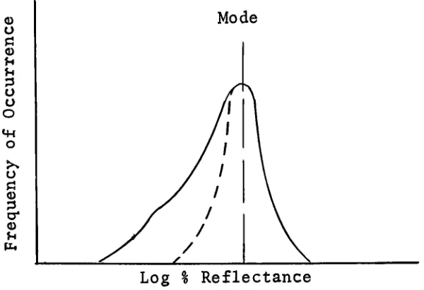
The

Figure

1.

PECULIAR

"HUMP"

SEEN ON

MANY

LOG E

DISTRIBUTIONS

Mean

o

pJ <D

U u o U o

o o

P5

c* <o u

tu

[image:11.548.113.494.169.598.2]

Sorem

et. al.2*3

in

1965

noted

the

"hump"

in many

of

their

log

luminance

distributions

and suggested

that

it

may

be

due

to

the

existance of shadows

in

the

scene.

If

indeed

the

existance of

the

"hump"

is

due

to

the

presence of

shadows,

then

it

is

entirely

possible

that

an aerial

distribution

contains

two

sets of

data...

one of objects

in

daylight,

the

other of similar objects

but

in

shadows,

both

mixed

together

and not

easily

distinguishable

in

the

collected

microdensi-tometer

data.

To

test

this

hypothesis,

there

are

five

(5)

methods:

1.

Photograph

an urban area when

the

sun angle

is

exactly

90

degrees.

This

would eliminate all shadows since

the

sun would

be

directly

overhead

and

the

distribution

should

be

symmetrical.

Unfortunately,

a

90

degree

solar altitude will not occur at

latitudes

greater

than

23

degrees

which makes

it

impossible

to

obtain aerial

photography

and still

stay

within

the

conti nental

United

States.

2.

Alternate

to

1.

is

to

obtain an aerial photograph

just

after sunset

to

give an urban area as all

"shadows".

Unfortunately,

this

would present a spectral

energy

distribution

unlike

that

during

the

day.

Nevertheless,

an attempt

to

obtain aerial

photography

at

dusk

was made

but

proved unfruitful

due

to

underexposure and

image

motion.

3.

An

aerial scene

with

and without shadows could

be

selectively

scanned so as

to

collect sunlit

data

points

separately

from

shadow

data

points.

A

gray

scale

in

the

shadows would allow proper

shadow reflectance conversion.

Unfortunately,

this

would require considerable micro-D operator

time

and

the

selection areas

may be

biased

to

4.

There

is

one specific case which at

first

thought

might

lend

itself

to

the

collection of

data

with

the

absence of shadows.

This

case exists

(other

than

for

case

1

above)

when

the

camera

pointing

vector

is

perfectly

aligned with

the

sun's

pointing

vector

(Figure

2)

.

This

situation

depends

strongly

on

the

time

of

day

and

is

very

difficult

to

obtain.

The

absence of shadows

would exist

only

in

a plane above

the

direct

line

of sight of

the

camera.

The

camera not

being

at

infinity

would see shadows

to

the

left,

right and

bottom

of

the

field

of view

making

this

technique

unacceptable.

5.

As

an asphalt road passes

from

sunlight

into

a

building's

shadow,

the

illuminance

changes

from

daylight

to

skylight.

The

aerial photo

graph,

in

recording

what

is

seen,

doesn't

discriminate

a

difference

in

illumination

from

a

difference

in

reflectance.

It

would

be

pos

sible

then,

to

statistically

analyze

log

exposure

distributions

in

terms

of

log

%

reflectance

(R)

distributions.

The

analysis would

test

each

distribution

for

normality

conjecturing

that

the

observed

log

%

R

distribution

actually

contains

two

separate

distributions

of:

a.

Sunlit

objects

b.

Similar

objects

but

in

shadows

Method

5

was selected

for

the

analysis and will

be

discussed

in

detail.

The

luminous

emittance

(M)

of an object

is

proportional

to

the

reflection

factor

of

that

object

(R)

times

the

illuminance

(I

)

incident

upon

it.

Any

change

in

illuminance

will result

in

a

direct

change

in

luminous

emittance of

that

object.

Therefore,

any

given

object will

have

a constant reflectance

providing

there

is

no change

in

the

direction

or

the

spectral

quality

of

the

illuminant.

This

paper

does

not attempt

to

consider

any

of

the

spectral variations of

daylight,

skylight,

objects,

and/or

their

relationships

to

each other.

Thus,

all

the

objects are considered as

being

gray

and

Lambertian

diffusors

as a good

first

order approximation.

Figure

2.

DEPICTS

CAMERA

LINE

OF

SIGHT

COINCIDENT

WITH

EARTH

-SUN

LINE

Sun

/

/

[image:14.548.109.419.383.725.2]

DISCUSSION

Experimental

Design

The

acquisition

planning

is

quite

important

to

successfully

perform

the

experiment.

Advance

consideration must

be

given

to

sun

angle,

camera

pointing

angles and

the

direction

of

the

shadows.

The

most

frequently

used aerial photographic

pointing

angle

is

straight

down

(vertical)

.

This

angle must

be

included

in

the

experiment as well as

photography

at angles other

than

vertical.

If

the

obliquity

angles

(angles

other

than

vertical)

are chosen such

that

they

look

at

building

sides

both

in

and

out of

shadows,

the

frequency

of

the

same object

both

in

and

out of shadows will

be

increased.

To

illustrate,

the

building

in

Figure

3

has

one side surface

illuminated

by

daylight,

and

the

other side

by

skylight.

The

road

by

the

building

is

in

daylight

as well as

in

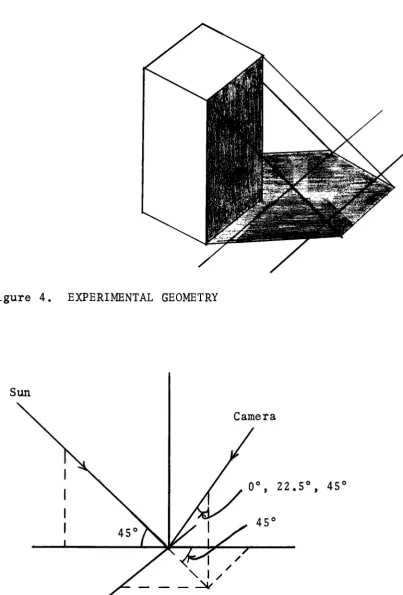
shadows.

The

camera

pointing

angles were selected

to

be

0,

22.5

and

45

degrees

from

vertical.

For

geometrical

reasons,

the

sun

angle at

the

time

of

photography

was selected

to

be

45

degrees.

The

projection of

the

camera's

line

of sight on

the

earth

formed

a

45

degree

angle with

the

projection of

the

sun's

vector on

the

earth

(Figure

4)

.

Two

replicates at each camera

Figure

3.

THE

SAME

BUILDING AND

ROAD ARE

SHOWN

WITH

TWO

TYPES

OF

ILLUMINATION

Figure

4.

EXPERIMENTAL

GEOMETRY

Sun

Camera

[image:16.548.61.465.119.715.2] [image:16.548.74.412.485.719.2]

To

accomplish

the

calibration and correlate

the

absolute

reflectance of ground objects

to

the

exposures received on

the

film,

a

five

step

gray

scale with

known

reflectances

was

laid

out on a

flat

ground surface.

Data Analysis

Only

those

processed negatives

that

contained

gray

scales

were selected

for

analysis.

The

same urban area was scanned

in

each

frame

selected

using

a

GAF

Model

650

microdensitometer.

The

scanning

process

is

similar

to

a

TV

raster such

that

data

are collected

automatically

in

lines

but

in

discrete

incre

ments as shown

in

Figure

5.

Figure

5.

RASTER SCAN

DEPICTING

COLLECTION

OF

DENSITY

DATA

POINTS

TOOOO^

Each

circle represents a

two

foot

ground area and

is

one

data

point.

The

output was

automatically

punched out on

computer cards

in

terms

directly

proportional

to

the

voltage

output of

the

microdensitometer.

The

process control

strip

with

known

densities

was also scanned with

the

microdensi

tometer

to

correlate

the

voltage output

to

density

and

ultimately

to

log

E.

Exacting

control was maintained

by

keeping

an undeveloped process control

strip

frozen

in

dry

ice

and removed at

the

end of

the

actual photography.

Any

latent

image

failure

that

occurred

to

the

flight

roll would

then

also occur

to

the

control strip.

A

computer program

then

generated a

frequency

histogram

in

terms

of

log

E

from

the

card

input

data.

Exposure

is

linearly

related

to

reflectance

by:

E

= _axR +

a2

where

E

= _{exposure received on}

the

film

R

= _{object reflectance}

a2

= _{a constant}

to

be

determined

by

linear

_regression

analysis and

is

the

intercept

of

the

exposure

axis where

the

reflectance

is

theoretically

zero.

a2

is

the

exposure

due

to

atmospheric

haze

luminance

which

is

non-image

forming

10

a.l

= _{a constant also}

to

be

determined

by

linear

regression and

is

the

actinic

transmission

factor

of

the

atmosphere.

If

the

transmit

tance

was

1.00,

the

slope would

be

45

degrees

and

a^

would

be

zero.

This

condition will

occur

only

in

the

absence of an atmosphere.

Five

large

gray

panels were placed

in

the

scene whose

reflectances were measured

by

a spectrophotometer.

The

spectral reflectance

data

was

integrated

over

the

same wave

length

region as

the

photography

and shown

in

Table

1.

The

five

step

gray

scale when photographed at altitude will

provide a method of

converting

the

log

exposures received

on

the

film

to

log

%

R

on

the

ground.

Table

1.

FIVE

STEP

GRAY

SCALE.

. .MEASURED

REFLECTANCES

AND

CORRESPONDING

FILM EXPOSURES

%

R

Log

E

E_

4.5

7.51

.0324

7.5

7.60

.0398

13.4

7.74

.0550

26.0

7.88

.0759

11

Figure

6.

LINEAR

REGRESSION

FIT

OF

TARGET

REFLECTANCES

TO

CORRESPONDING

EXPOSURE

RECORDED

ON

FILM

U

o

X

VI

.12C

-.100

-.060

-.040

"

.020

-Regression

Intercept

Regression

Slope

.027100

.001817

10

20

30

I

Reflectance

T"

[image:20.548.44.530.131.713.2]

12

The

equations'*

used

in

the

regression are:

5ZER

-

SEER

*,-..,

a, =

; = .001817

1 5ZR2

- (ZR)2

a _

SESR2

-

ZERZR

n,,in.

&2

"

5ZR*

-(ZIP

=

-027100

The

regression

line

and actual

data

point

fit

are shown

in

Figure

6.

The

log

E

distribution

may

now

be

converted

to

a

log

%

R

distribution.

To

test

the

theory

proposed

in

the

introduction

that

there

are

in

actuality

two

distributions,

the

statistical analysis

begins

by

folding

the

upper

distri

bution

data

about

the

mode such

that

a symmetrical

distribution

is

formed

as shown

in

Figure

7.

The

folded

distribution

is

subtracted

then

from

the

total

distribution

to

produce

a remainder or "shadow"

distribution

shown

in

Figure

8.

A

special computer program was written

to

do

the

manipulations

as well as perform

the

statistics.

Chi-square

tests

to

check

for normalcy

were performed on

the

total,

folded

and "shadow"

13

Figure

7.

UPPER PORTION

OF

DISTRIBUTION

FOLDED

ABOUT

MODE

Log

%

Reflectance

Fieure

8.

FOLDED

DISTRIBUTION

SUBTRACTED

FROM

TOTAL

-DISTRIBUTION

TO

GIVE

"SHADOW"

DISTRIBUTION,

EXAGGERATED

Mode

[image:22.548.142.442.150.355.2]

14

RESULTS

The

results are summarized

in

Table

2

for

each

distribution

A

through

F

making

a

total

of

18

distributions

evaluated.

The

hypothesis

that

the

distributions

are normal

is:

H

:

(0

- E)2 _-.

0

null

hypothesis

Ht:

(0

- E)2 _>

0

_{alpha risk} =

.10

where:

0

is

the

observed

frequency

E

is

the

expected

frequency

To

interpret

the

statistics pf

Table

2,

the

last

column shows:

1.

None

of

the

distributions

from

the

vertical

photography

are normal.

2.

Some

of

the

distributions

are accepted as normal

for

the

side

looking

photography

(22.5 and

45).

The

statistical acceptance means

there

is

no

reason

to

believe

that

the

distributions

are

not normal.

3.

It

appears

that

there

is

a

larger

incidence

normalcy

at

the

larger pointing

angles (45 as opposed

to

22.

5)

.

The

hypothesis

then

implies

that

there

are

indeed

two

distri

butions;

one of objects

in

sunlight and

the

other of similar

objects

but

in

shadows.

There

was one assumption made

that

may have

altered

the

results

In

every

case

the

distributions

were

folded

about

the

mode.

16

Table

2.

STATISTICAL

COMPARISON OF

TOTAL,

FOLDED AND SHADOW

DISTRIBUTIONS

Angle

of

View

Di

stribution

Calculated

x2

Degrees

of

Freedom

Table

X2 ~

51.8

34.4

37.9

Based

on

Null

Figure

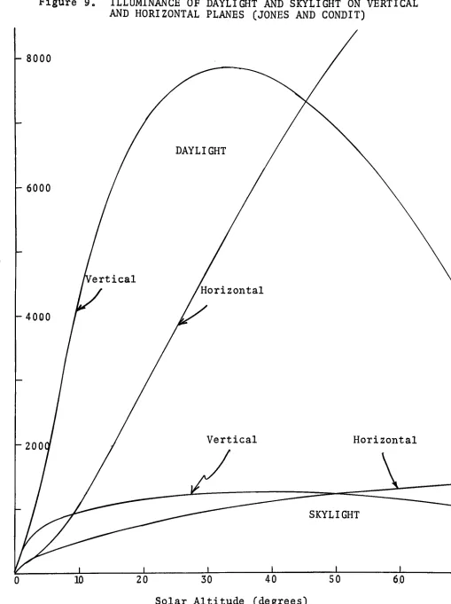
9.

ILLUMINANCE

OF

DAYLIGHT

AND SKYLIGHT ON

VERTICAL

AND

HORIZONTAL

PLANES

(JONES AND

CONDIT)

17

-

8000

-DAYLIGHT

/

-6000

/Vertical

/Horizontal

-4000

-200QT

Vertical

Horizontal

i i i i

SKYLIGHT

10

20

30

40

Solar Altitude

(degrees)

[image:25.548.18.527.62.743.2]

15

mean often

lies,

far

enough

from

the

mode

to

make

the

folded

distribution bi-modal

and

the

"shadow"

distribution

negative.

It

is

believed

that

the

mode was a good choice.

Table

2

shows

that

none of

the

vertical

distributions

are

normal.

A

reason

may

be

that

in

the

vertical

photography,

the

roofing

material

of a

building

in

sunlight

may be

different

than

one

in

shadows.

Whereas,

in

the

side

looking

photography,

the

same

building

could

be

in

a shadow as well as

in

sunlight

(as

shown

in

Figure

3)

.

The

side

looking

photography

would

have

a

higher

incidence

of similar objects which

may be

significant.

To

further

substantiate

the

above

possibility,

an adjustment

of

the

"shadow"

distribution

may

be

made

for

the

difference

in

daylight

to

skylight

illumination.

Jones

and Condit5

report

the

data

shown

in

Figure

9

and show a

log

ratio of

1.2:1

at

45

degrees

sun angle.

Inasmuch

as

the

distributions

are normal at

the

larger

pointing

angles,

only

the

means

need

be

compared.

The

question

is

then:.... Is

the

shadow

object mean reflectance similar

to

daylight

object mean

reflectance when

its

illumination

is

adjusted

to

be

the

same as

daylight?

As

a

hypothesis...

H0

H

shadow

=

y

daylight

H:

y

18

The

test

statistic

is:

(*i

-%2)

-CUx

-U2)

a rxp

(xT

-x2)

where:

Pi

-U2

=

₀

a

_

=

sD

-yTl

l

(xx

-x2)

p

v +

ir:

As

is

shown

in

Table

3,

for

01 =

.05 and

t

=

1.96,

the

student

t

values are quite

high.

Therefore,

it

is

not possible

to

reject

the

null and

the

hypothesis

that

the

means are

the

same

is

true

to

within

95%

probability.

Therefore,

there

is

no evidence of signi

ficant

difference

in

the

two

averages compared and

the

objects

19

Table

3.

STATISTICAL

COMPARISON OF

FOLDED

AND

SHADOW

DISTRIBUTIONS ADJUSTED FOR

DIFFERENCES

IN

ILLUMINATION

Distribution

Mean

s

Adjusted

n

s

a(~

7

-^

Log

%

R

Means

P

(Xl

'

*z)

Log

%

R

D

Folded

1.39

0.14

1.39

201

,

.165 .0192

20.8

D

Shadow

.99

0.19

1.20

117

E

Folded

1.44

0.08

1.44

56

.085 .0129

11.6

E

Shadow

1.29

0.09

1.56

190

F

Folded

1.53

0.09

1.53

57

.10 .0147

12.9

20

CONCLUSION

Log

%

reflectance

distributions

obtained at

obliquity

angles

greater

than

22.5

degrees

contain

two

log

normal

distributions

One

that

contains objects

in

daylight

and

the

other

that

contains similar objects

in

the

shadows.

The

difference

is

apparently due

to

a

difference

in

illuminance

and

the

statistics show

that

the

ratio of

the

two

distributions

are

21

REFERENCES

1.

Mees,

C.

E.,

The

Theory

of

the

Photographic

Process,

Macmillan Co.

,

New

York,

1954.

''

2.

Sorem,

A.

L.,

Fritz,

N.,

Speckt,

R.

,

"Luminance

Distributions

in

Aerial

Scenes",

S.P.S.E.

Convention,

May 17-21,

1965.

3.

Sorem,

A.

L.,

"Luminance

Characteristics

of

Aerial

Scenes",

Part

I.,

S.P.S.E.

Convention,

April

29,

1963,

4.

Rickmers,

A.

D.

and

Todd,

H.

N.

,

Statistics:

An

Introduction,

p.

251,

McGraw-Hill

Book

Company,

Inc.

New

York,

1967.

5.

Jones,

L.

A.

and

Condit,

H.

R.

,

"Sunlight

and