RESEARCH ARTICLE
Integrating text mining, data mining,
and network analysis for identifying genetic
breast cancer trends
Gabriela Jurca
1, Omar Addam
1, Alper Aksac
1, Shang Gao
2, Tansel Özyer
3, Douglas Demetrick
4and Reda Alhajj
1,5*Abstract
Background: Breast cancer is a serious disease which affects many women and may lead to death. It has received considerable attention from the research community. Thus, biomedical researchers aim to find genetic biomarkers indicative of the disease. Novel biomarkers can be elucidated from the existing literature. However, the vast amount of scientific publications on breast cancer make this a daunting task. This paper presents a framework which investigates existing literature data for informative discoveries. It integrates text mining and social network analysis in order to identify new potential biomarkers for breast cancer.
Results: We utilized PubMed for the testing. We investigated gene–gene interactions, as well as novel interactions such as gene-year, gene-country, and abstract-country to find out how the discoveries varied over time and how overlapping/diverse are the discoveries and the interest of various research groups in different countries.
Conclusions: Interesting trends have been identified and discussed, e.g., different genes are highlighted in relation-ship to different countries though the various genes were found to share functionality. Some text analysis based results have been validated against results from other tools that predict gene–gene relations and gene functions. Keywords: Breast cancer, Data mining, Text mining, Network analysis
© 2016 Jurca et al. This article is distributed under the terms of the Creative Commons Attribution 4.0 International License (http://creativecommons.org/licenses/by/4.0/), which permits unrestricted use, distribution, and reproduction in any medium, provided you give appropriate credit to the original author(s) and the source, provide a link to the Creative Commons license, and indicate if changes were made. The Creative Commons Public Domain Dedication waiver (http://creativecommons.org/ publicdomain/zero/1.0/) applies to the data made available in this article, unless otherwise stated.
Background Introduction
CANCER is one of the most serious and harmful diseases threatening humanity and may lead to death. Unfortu-nately there is no discovered robust treatment which leads to guaranteed cure from cancer. Thus, researchers from various domains are still working hard to identify molecules (mainly genes or proteins) which could be han-dled and targeted as cancer biomarkers. Various methods have been developed. The research spans a wide range of techniques from wet-lab testing by biologists to com-putational methods by computer scientists. The latter research is promising because it helps in tremendously
reducing the number of molecules to consider as poten-tial biomarkers.
Cancer is a result of damage (mutation) to a cell’s DNA (deoxyribonucleic acid), so that the cell loses normal functionality and instead gains the ability to indefinitely multiply until normal tissue functions are impaired [1]. Cancerous DNA mutations may occur from a complex mixture of inherited and external (environmental) fac-tors, where these mutations are usually located in cell division genes [1]. There are over 100 known different types of cancer, depending on the cell type which was originally affected [1]. Additionally, each patient may have a different set of cancerous mutations in various genes, which may lead to different subtypes of the cancer. In order to personalize therapeutic strategies for cancer patients, medical researchers aim to identify and char-acterize the biomarkers of each type of cancer, so that they can provide the most accurate diagnosis to patients
Open Access
*Correspondence: [email protected]
1 Department of Computer Science, University of Calgary, Calgary, AB, Canada
Page 2 of 35 Jurca et al. BMC Res Notes (2016) 9:236
[2]. A cancer biomarker refers to a substance or process that serves as indication of cancer in the body, where one common example of a cancer biomarker is genetics [3].
The basic unit of genetic biomarkers are genes. A gene is one unit of the DNA which often contains the informa-tion needed to produce proteins. The central dogma is that genes are transcribed into an intermediate molecules called RNA, and the RNA is then translated into proteins, where proteins carry out the basic functions of life [4]. If a gene codes for a protein whose function is to suppress cancer, then if that gene is damaged or is downregulated (not transcribed enough), then the cell may become can-cerous. Similarly, if a gene codes for a protein whose func-tion is to promote cancer, then if that gene is upregulated (transcribed more than usual), then that cell may also become cancerous. Therefore, finding the different genes and conditions which are likely to lead to cancer, should the genes be upregulated or downregulated, is an impor-tant task for characterizing types of cancer. The problem is not trivial because there are various internal and exter-nal factors that might affect the cells leading to cancer. People do not have the same habits and behavior. Thus they may develop the same cancer differently based on the environment they live in, their diet, drinking, etc. Also, some types of cancer, such as breast and prostate cancer can be strongly influenced by inherited gene mutations, and often run in families [5]. Therefore, these heritable types of cancer may be predicted by examining a person’s DNA before they develop cancer. Identifying the heritable genetic mutations that increase the likelihood for cancer are critical to developing predictive genetic tests.
Our framework described in this paper is built on the hypothesis which could be articulated as follows. To investigate cancer biomarkers, one may investigate the literature which contains a huge amount of informa-tion hidden in the form of scientific articles. However, a query for “breast cancer” to PubMed can retrieve over 250,000 articles, which makes it impossible to get a full-picture of the field by reading them. The trend is that the number of PubMed articles are steadily increasing, and so are articles on the topic of breast cancer that mention gene names argued as potential biomarkers (see Fig. 1). Therefore, using text mining techniques to gather new knowledge from many existing scientific sources can be an effective way to investigate the literature for new bio-markers. One type of relationship which can be discov-ered is gene-disease, that shows which gene is involved in which disease [6]. Another type of relationship which can be found are gene–gene interactions [7].
Some data mining techniques that can be used to extract hidden information from a database are hard clustering, soft clustering, hierarchical clustering, and frequent pattern mining [8]. All of the aforementioned
techniques are described in more detail in “Results and discussion” section. Each data mining technique uti-lizes different interestingness metrics, so it is useful to apply many techniques to a data set. Another technique we used on the genes extracted from the breast cancer abstracts was network analysis, or “Social Network Anal-ysis” as it is sometimes referred to [9]. Network analysis has its roots in sociology, as it was first used to study the relationships and community structures in social data. However, network analysis has since been applied in other fields such as bioinformatics in order to find key molecular markers and communities within an interac-tion network.
To validate genes linked to cancer, one of the most effective ways is to analyze disease specific gene expres-sion data [10].
Gene expression data is experimental data which can be used to check whether a gene has indeed been upregulated or downregulated with respect to a dis-ease. This methodology compares to what level genes were expressed in cancerous cells versus healthy cells. It is unaffordable and infeasible to try wet-lab analysis of such a huge set of genes. Therefore, machine learn-ing and data minlearn-ing techniques (includlearn-ing frequent pat-tern mining, clustering and classification) can be used to lower this number of genes down to a manageable set of genes which are anticipated to be statistically linked with the disease. This way, biologists will concentrate only on the identified small set as potential cancer bio-markers instead of unrealistic case of testing every gene in the wet-lab as potential cancer biomarker. In other words, data mining techniques can save the time and cost of cancer researchers, turning their research goals into something potentially achievable. This is illustrated by the test results reported in this paper.
The paper is organized as the following sections. The problem explanation is made in “Problem explana-tion” section. “Related work” section describes the work
related to our solution. In “The developed solution” sec-tion, the developed methodology is given in detail. The experimental results are depicted in “Evaluation of the developed solution” section. Lastly, contributions and future work are mentioned in “Results and discussion” section.
Problem explanation
Identifying cancer biomarkers is not a trivial task. Despite all the effort, time, and money invested so far, the progress is still very little. Indeed the body is affected by various internal and external factors which altogether may lead to cancer. As the factors differ from person to person, the samples taken from two cancer patients may not reveal exactly the same information. Thus, there is a need to develop new techniques which could better ana-lyze the existing sources of data with the hope to lead to more useful discoveries.
In this paper, we aimed to perform large-scale text analysis of biomedical abstracts in order to generate new hypothesis about cancer biomarkers. The target was to develop a data mining methodology, which would lead to patterns in the genes which are associated with cancer. In the this section we will discuss the tasks involved in text mining.
Text mining
Text mining is typically comprised of four stages [11,
12]: (1) information retrieval (IR), where a set of textual materials are gathered for a given topic; (2) entity recog-nition (NER), where textual features are identified from the gathered texts; (3) information extraction (IE) which aims to extract relationships among the recognized tex-tual features; (4) knowledge discovery (KD), where the extracted relationships are used to identify useful pat-terns from the data set. The rest of this section is dedi-cated to explain each stage and how they can be applied to biomedical text mining.
Information retrieval for text mining The first step in text mining is to gather the papers which are relevant to the topic of interest. There are a number of IR systems, including centralized institutional like PubMed and UK PubMed Central (UKPMC), or commercial systems like google scholar. The best known one is PubMed [11–13], which searches the MedLine database.
First, we can categorize an IR engine by the input. The topic may come from a query provided by the user, and this method of defining the topic is called ad hoc [14]. The other kind of IR system is called text categorization, where the input is a set of papers. Ad hoc has some limi-tations compared to text categorization [13]. PubMed is an ad-hoc system. Second, we can also categorize IR
engines in terms of the scope of content delivered. For example, PubMed produces a comprehensive search of articles, but only retrieves the abstracts of the articles. In contrast, UKPMC returns the full text of articles [13].
Entity recognition (NER) Once we have a subset of the available scientific literature which pertains to our topic, we must identify terms which are relevant to our study. NER has the aim of identifying terms within the gathered text, such as the names of different proteins or genes. The first task of these systems is to identify the biologi-cal entity names. The second task of NER is to identify the unique entity names. However, identifying biological terms is challenging due to the following reasons [12]:
• Biomedical terms often have synonyms (e.g., PTEN
and MMAC1 refer to the same gene).
• A term may have different meanings (e.g., Cancer can
also mean the astrological sign).
• Acronyms may lead to ambiguities (e.g., BC may
mean breast cancer or it may mean British Colum-bia).
These challenges can make the naming of the biologi-cal entities quite imprecise. However, some strategies to overcome these drawbacks have been implemented in NER systems. One method is to integrate different vocabularies and ontologies which hold complete lists of biological entity names [12]. For example, gene ontology is a classification effort to describe what we know about genes, including to develop controlled vocabularies about those genes.
Early NER systems were rule-based with manually designed rules based on word structures. More recently NER systems have shifted to machine learning tech-niques which can recognize characteristics of words. A third type of NER systems is dictionary-based, which is the most effective due to the fact that it can recognize synonyms. In addition, it is also possible to use algo-rithms which can disambiguate acronyms automatically [11]. Some examples of NER systems that recognize bio-medical entities are NCBO annotator, cTAKES, Meta-Map, and BeCAS. A study which compared these four systems using their own ground truth determined that BeCAS performed differently compared to the other three systems [15]. BeCAS performed more poorly over-all, but BeCAS recognized larger sentences than the other systems, which may have been underrepresented in their evaluation [15].
Page 4 of 35 Jurca et al. BMC Res Notes (2016) 9:236
label proteins and genes, followed by verification with the UniProt database using the given UniPROT ID. UniProt is a database which stores genes and proteins information.
Information extraction (IE) The aim of IE is to extract relationships between the biological entities mentioned in the text. There are two approaches for this: co-occurrence processing and natural language processing (NLP) [11]. In co-occurrence processing, the entities are deemed to be related if they occur in the same text. For example, the relationships found are usually of the type gene–gene, or gene-disease. However, in co-occurrence processing, one cannot extract directional relationships between entities.
Through NLP, the directionality of the relationship between the biological entities can also be found. NLP analyzes the syntax and semantics of the sentence which contains the entities. However, NLP is better suited for full-text mining rather than abstract mining. The con-cise nature of abstracts makes it difficult to analyze the context of the biological entities [14]. Also, due to their complexity, NLP systems are designed for limited and specific types of relationships, and only a few systems can
recognize multiple types of relationships [14]. As further discussed in “The developed solution” section, we used BeCAS API [16] to annotate and extract co-occurrences of biomedical concepts such as gene, protein, etc.
Knowledge discovery (KD) KD is the extraction of knowledge from a large volume of structured and/or unstructured data. The goal of KD is to uncover novel knowledge from existing data. Novel data can be in the form of hidden relationships among biological entities. For example, if A is related to B, and B is related to C, text mining can infer the relationship that A is related to C. It is difficult for people to discover indirect relationships from a large amount of data. KD is often used to gain biologi-cally meaningful knowledge about how biological entities are related.
Hypothesis generation
One of the newer approaches described in the literature is to generate scientific hypotheses through text mining [11, 13]. KD can be used to generate scientific hypoth-eses, for example about relationships between entities, which have yet to be validated. Whereas KD attempts to discover biological meaning about a set of facts, hypoth-esis generation attempts to discover whole new relation-ships. Hypothesis generation can be useful at directing scientists to which genes they should study without wast-ing much resources on the exploration.
The work described in [11] describes two ways in which hypothesis generation can occur: one way is to start with the microarray data to identify genes hypotheses, and then to support these hypotheses with literature mining. The second is to generate hypotheses through literature mining, and then validate the hypotheses through experi-mental data, such as microarray data. We decided to investigate the second method of hypothesis generation; actually, Faro et al. [11] identified the field as more lack-ing in research.
Evaluation
Some related work that use biomedical text mining to generate hypotheses have evaluated their results with experimental data [11, 17]. Experimental data can consist of gene expression data, which often comes in the form of microarray data. Gene microarray experiments are per-formed using specific tissue samples, and they measure the presence of the intermediate molecule RNA, so that we can know which genes are important in particular conditions [18]. Some genes may be up- regulated, which means that they were transcribed more, and we say that these genes were ‘expressed’. Otherwise, the genes may be down-regulated, which means that the genes were not ‘expressed’. Genes that were expressed together at the
same time may have a relationship together, and we say they are ‘co-expressed’.
There are publicly available online repositories that store experimental data, as well as the gene–gene rela-tionships and gene functionalities derived from experi-mental data. Some tools such as GeneMania have been built that show the relationships between genes by inte-grating information from various databases [19]. Tools such as GeneMania may be useful for validating the gene–gene relationship hypotheses. There are also tools such as DisGeNet [20, 21] and FunDo [22] that identify gene-disease relationships from curated sources.
Related work
Faro et al. [11] described the methodology of hypothesis generation from literature, combined with experimental data evaluation, to be quite novel in 2011. In this section, we will describe some of the tools and methodologies which have been used for hypothesis generation from biomedical literature.
GeneWizard is an application which allows users to generate biological hypotheses based on text mining, and then evaluate the hypotheses through gene expres-sion data [17]. One advantage of this tool is that it can be used to generate hypotheses about genes of any disease, whereas our methodology has so far been focused on breast cancer. However, in the future we aim to try our methodology on other cancer or diseases as well.
For the IR step, GeneWizard also used PubMed to retrieve articles related to the disease of interest, just as we did in our methodology. For NER, GeneWizard recog-nizes the biological entities related to a disease by using dictionaries created for the disease and for the genes. To identify relationships between genes, GeneWizard performs clustering of the abstracts, based on similarity matrices constructed from abstracts, based on the fre-quencies of the disease and gene terms.
Another goal of GeneWizard is to be highly usable, so that not much experience with text mining methods is required of the users. Faro et al. [11] stress that it is important for tools that generate biological hypotheses to have a high usability, since the audience who use these tools are likely to be biologists, not computer scientists.
Another tool is called BioWizard, which is very similar to GeneWizard, yet it performs full-text analysis instead of abstract analysis [23]. Also, BioWizard was tested against gold standard gene-disease relationships in order to check the precision of the recall, in addition to experi-mental data in the form of microarray data. This system was then moved to the cloud in order to perform more intensive computations in a shorter amount of time [24].
Another study which generated hypotheses from litera-ture performed the IE step by splitting the abstracts into
sentences and considered the sentences which contained an interaction plus two gene names [25]. A network of genes was built from the extracted genes and interac-tions. The genes which ranked the highest in centrality measures were manually validated by looking through literature. A similar study was done by [6], and high accu-racy was achieved for finding actual gene-disease rela-tionships in prostate cancer. Interestingly, even genes which were missed later turned out to have an article written about how they were indeed involved in prostate cancer [6].
Our contribution is that we will use different data min-ing techniques and various APIs for the different stages of the text mining, and that we will investigate relationships such as gene-country, gene-year, and abstract-country which have not been investigated by other papers so far. We explored how these new types of relationships can help to generate hypotheses about which genes should be studied.
Methods
The developed solution Overview
Figure 3 illustrates the steps of the methodology. Our goal is to contribute novel ideas for KD and hypothesis generation related to genes involved in breast cancer. We decided to use ready-API’s for IR, NER, and IE parts of the developed framework. The first step in our solution was the IR step, where our goal was to retrieve all rele-vant papers related to our topic of interest: breast cancer.
Page 6 of 35 Jurca et al. BMC Res Notes (2016) 9:236
was excluded, 62,752 papers did not have an abstract and 257 did not have a date.
The PubMed API also provided extra information about the articles, such as keywords, title, abstract, authors, affiliation of authors, publishing date, and journal name. In addition to the abstracts, it was useful to receive most of the extraneous data in a standardized format, because we could use it to perform additional analysis on breast cancer data. However, not all of the data was clean and therefore they required more processing, such as author affiliation. We will later discuss how we processed author affiliation in order to use it for the analysis. In the next step, we recognized the named entities in the abstracts and titles. We used an online API called BeCAS, which identifies biomedical concepts in text [16]. In our opin-ion, BeCAS is a well-documented API; it performs well enough at identifying biomedical terms. Further, another important reason for using BeCAS was because it is inte-grated with PubMed such that it requires only the Pub-Med ID of the abstract in order to perform the analysis.
Thus, we did not need to upload the abstract itself into BeCAS. This saved computational memory and time.
The named entities we were interested in are genes and proteins. Since we wanted to consider only genes for our analysis, we collected the genes from the text, but we also collected genes which were associated with proteins that were mentioned in the text. Another reason for using BeCAS is because it is well-integrated with the UniProt database [26] which stores genes and proteins informa-tion. For each protein and gene, BeCAS provided the Uni-Prot ID in order to verify the entity. The UniUni-Prot ID also allowed us to retrieve genes which were associated with the proteins mentioned in the text. UniProt also helps to address one of the biggest challenges in biomedical text mining, i.e., genes may contain many synonyms. UniProt stores known synonyms for each gene name. This helps to reduce the number of duplicate genes listed within the abstracts under alternative names. After recognizing genes within the abstracts as well as those associated with the proteins mentioned in the abstracts, we filtered the paper
set to include only abstracts which contain genes. There-fore, our final paper-set used in the analysis was reduced to 117,339 papers. The abstracts which were excluded follow-ing the NER step may be related to other aspects of breast cancer, possibly from a health care or psychological per-spective, not the genetic side which we are interested in.
The next step was to generate hypotheses about the relationships between genes, and also between genes and other information associated with them, such as the abstracts and authors. The relationships between the genes were measured as co-occurrences within the abstracts, and the semantic relations or directionality between the genes were not extracted to be used in the analysis. Although many hypothesis-generating methodologies use gene–gene relationships to generate hypotheses about which genes should be investigated, our methodology uses additional information, such as the authors, locations, and dates. Therefore, we developed a methodology to create hypotheses that stem from different types of information that is typically used by other researchers.
One of the features that we examined was the country of an author’s affiliation. By extracting the country of an author’s affiliation, we then related the countries which published breast cancer papers to the genes. Interesting correlations were then found, such as the genes that par-ticular countries focused on. Researchers might use the gene-country information to see which genes are hot top-ics to study in a country. Another feature that we consid-ered was the year that the abstract was published in. The gene-year relationship allowed us to find which genes were frequently mentioned together every year, which might lead a researcher to believe that these genes might have a hidden connection that needs to be further explored in the wet-lab. A third relationship that we explored was gene–gene co-occurrence frequency within the abstracts. An ideal analysis technique to explore the gene–gene rela-tionships was network analysis, as the genes could be the “actors” and the number of abstract co-occurences could be the “action” between two genes. The network analysis technique is further discussed in “Results and discussion” section. Lastly, we also examined how many abstracts each country published in order to find which countries are the top contributors to breast cancer research.
For the data mining analysis, we used the software KNIME.1 For the social network analysis, we used Gephi.2 The web tools that we used to evaluate some of our results were GeneMania, DisGeNET, and FunDO. The computer used for the analysis has the following main specifications: Intel i5-4570 CPU, 8gb RAM, Win-dows 10 OS.
1 http://www.knime.org (last visited 24 Nov 2014). 2 http://gephi.github.io (last visited 24 Nov 2014).
Country identification
To find countries associated with each retrieved arti-cle, we needed to process the string which contains the affiliation(s) of authors, called the position (Fig. 4). The extra processing was required because the position often contained extraneous information, such as the names of the institution(s) and the author’s e-mail. The number of authors was around 500,000, but after we grouped them by first name, last name, and affiliation, the number rose to 601,287, most likely due to authors changing institu-tions throughout their careers or having popular names referring to different authors at different institutions, e.g., ‘Ken Barker’ is a popular name who exists at three insti-tutions. There were 193,000 different possible affiliations for the authors who published abstracts with genes men-tioned in them. Many authors contained multiple institu-tions in their affiliainstitu-tions.
For each of the affiliations, we then wanted to find the associated country name. We used google maps API3 to retrieve the country name. We split the string into sub addresses using the comma delimiter. Each search was performed using the rightmost delimited address, which often contained the country name. However, when the sub address string was insufficient to achieve exactly one coun-try name, we repeatedly increased the size of the string with the next rightmost element of the sub address. As seen in Fig. 4, we first made a query using sub address 1, and if that did not return precise enough results to reveal the country of origin, then we made another query which also included sub address 2, etc. The final set excluded all of the institutions inside each affiliation which did not con-tain a valid address, which was about 1 %. One limitation of google maps API is that it had a daily quota of queries which could be submitted to the service. With our large number of institutions, we needed to optimize the number of online queries. We achieved this by constructing a cache system which stored all special keywords existing in the affiliations; this helped us to distinguish the institutions directly. Using the cache system, we submitted only 8558 queries to google maps API. Altogether, we found that there were 159 countries with articles published under “breast cancer” category and contain genes.
Results
Evaluation of the developed solution Overview
Our gene–gene results were evaluated by comparison to results retrieved through a web tool called GeneMania4 which uses publicly available curated and experimental
Page 8 of 35 Jurca et al. BMC Res Notes (2016) 9:236
data to derive gene–gene relationships [19]. GeneMania also shows predicted relationships [19]. If most of the relationships that we hypothesize are also reported by GeneMania, then our hypothesis would be strengthened. Any gene–gene relationships that are missing in the GeneMania results have the potential to be newly discov-ered relationships that may warrant more investigation by wet-lab researchers.
Our gene-disease results were evaluated by comparing our results to DisGeNet and FunDo, which are two web tools that identify gene-disease relationships.
Resources used
Evaluation of gene clusters and communities For the evaluation of our results, we used GeneMania in order to
link our text-mining results to results drawn from experi-mental data [19]. GeneMania accounts for a few different types of interactions between genes, such as co-expres-sion, physical interaction, genetic interaction, shared protein domains, co-localization, pathway, as well as pre-dicted relationships using orthological functional data from other organisms. For all of our evaluations, we used datasets that described human genes.
Co-expressed genes are genes which had the same expression levels over the same conditions in a published study, where most of the gene expression data came from the gene expression omnibus (GEO) database. Another interaction in GeneMania is physical interaction, which means if two genes code for proteins that have a physical interaction, then the two genes have a connection. These
protein–protein interactions were pulled from BioGRID5 and pathwaycommons databases, which store protein– protein interactions. The other interactions we consid-ered from GeneMania were shared protein domains, Co-localization, and pathway interactions. Two genes partake in the shared protein domain interaction if their proteins have the same protein domain. Two genes have co-localization interaction if their proteins are found in the same body tissue. Finally, two genes share in the path-way interaction if they participate in the same reaction in a pathway. The sources of data that GeneMania uses are listed in the highly cited published paper [19].
Disease identification To find the disease which was most associated to each gene, we used the DisGeNET6 API [20, 21]. DisGeNet finds gene-disease relationships, from either curated sources, literature based associations, or predicted associations. For our study, we were inter-ested only in human gene-disease relationships, so there-fore we only used the curated sources. The curated sources for DisGeNET include human gene-disease relationships from the comparitive toxigenomics database (CTD) and UniProt. We used DisGeNET to find the gene-disease associations for the genes found through the gene-year and gene-country clustering (Appendix: Tables 9, 10). The diseases were identified on a gene by gene basis.
For the social network analysis, we used FunDO7 to identify the diseases which were common between large groups of genes [22]. FunDO takes a list of genes and retrieves the related diseases, based on the disease ontol-ogy database. The reason that we used FunDO instead of DisGeNET for analyzing the gene communities, is that FunDO provides a better analysis for common diseases between a group of genes. DisGeNET provides exclusive lists of diseases for each gene, whereas FunDO provides a list of shared diseases among the genes. An automated identification of diseases shared among groups of genes was beneficial, because the smallest community we obtained had 229 genes in community 1 (Appendix: Table 8). For each community from the social network analysis, we retrieved the top five diseases within the community.
Discussion
Results and discussion Hard clustering
Clustering is the process of grouping items together into “clusters”, so that the items within each cluster have more similarity to each other than to items in other clusters.
5 http://thebiogrid.org (last visited 24 Nov 2014).
6 http://www.disgenet.org/web/DisGeNET/v2.1 (last visited 24 Nov 2014). 7 http://django.nubic.northwestern.edu/fundo (last visited 24 Nov 2014).
Hard clustering separates items into distinct groups, where each item belongs to exactly one cluster. We per-formed hard clustering on genes with respect to the country affiliation of the authors who published papers on the genes. In this section, we present our results and some of the interesting genes a researcher might find to study from the results.
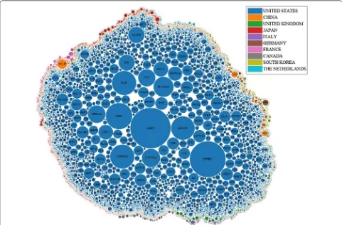
Which countries have studied the largest number of breast cancer genes? In Table 1, the country which published the largest number of articles on the topic of breast can-cer is the United States; authors affiliated with the United States also published the largest number of articles which mention breast cancer genes. In Fig. 5, the genes were clustered by colour of the countries that published the most amount of papers on those genes. Figure 5 shows that the United States has studied the largest number of genes by far, since most of genes have been mentioned by abstracts affiliated with the United States. Countries which ranked second and third are China and United Kingdom respectively. The United States, United King-dom, and China seem to have the largest support for breast cancer research and are leading the research worldwide.
In general, the difference between the top countries which published articles pertaining to breast cancer was not very different from the top countries which published articles containing breast cancer genes. Therefore, in these top countries, the molecular side of breast cancer was just as studied as are other aspects of breast cancer; this shows the importance of genetics in breast cancer research.
Collaborations We assume a collaboration if a paper had affiliations with institutions in different countries. The number of collaborations between countries on arti-cles which had to do with breast cancer occurred most
Table 1 The number of gene mentions
All Abstracts Abstracts with gene mentions
United States 62,013 United States 33,373
United Kingdom 11652 China 6553
China 8858 United Kingdom 6041
Japan 8807 Japan 5299
Italy 8667 Italy 4621
Germany 7394 Germany 4148
France 6757 France 3642
Canada 6476 Canada 3573
The Netherlands 4071 South Korea 2144
Page 10 of 35 Jurca et al. BMC Res Notes (2016) 9:236
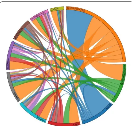
likely between United States and China (see Fig. 6). How-ever, when we considered collaborations on articles which mentioned breast cancer genes, countries which had the largest number of published articles such as United States, United Kingdom, and China had a slightly lower number of collaborations. However, countries with a lower amount of publications had more collaborations than before (see Fig. 7). Collaboration information allows researchers to recognize countries which are most involved in research as a partnership with others.
What are the top studied genes in the breast cancer field? Researchers may want to know the top studied genes in the breast cancer field, so that they may focus their research on promising genes. The top two most mentioned genes in the breast cancer abstracts were ESR1 and ERBB2 (Fig. 8). The next five most studied genes were EGF, PGR, CDKN2A, BRCA1, and SLC20A2 (Fig. 8). In total, there were 21 unique genes, when we considered the top 10 most studied genes for the top 10 countries
Fig. 5 The top 500 most frequently mentioned genes are shown, where radius represents the number of abstracts which mentioned the gene, and the colour represents the country which mentioned the gene the most
[image:10.595.57.538.88.405.2] [image:10.595.305.539.458.678.2]in breast cancer research. Related to these genes, more detailed information is listed in Appendix: Table 11. How-ever, please note that the curated source from DisGeNET did not contain information for CEAMC3, MUC21, and DHPS.
To measure the amount of effort that a country X put into a gene Y, we divided the number of abstracts from country X which mentioned gene Y, by the number of papers published from country X. All of top 10 countries for breast cancer research put most of their effort into ESR1 and ERBB2 (Fig. 9). Gene ESR1 received 11–20 % of the effort, with the United Kingdom contributing the highest effort. Gene ERBB2 is contained in 9–17 % of the effort, with France contributing the highest effort. For all the 21 unique genes, the effort ranged from 2–20 %.
Unsurprisingly, the protein products of ERBB2 and ESR1 are targets of drug and hormone therapy for breast cancer.
ERBB2, popularly known as HER2, codes for a recep-tor tyrosine-protein kinase, which is found in membrane signaling complexes, and facilitates the transmission of cell messages [27]. If ERBB2 is over-expressed, then the cell may get too many messages to proliferate and to survive, which may lead to breast cancer. Breast cancer patients which are ERBB2 positive (30 % of patients) can be treated with the medication trastuzumab, with the trade name Herceptin [28].
On the other hand, ESR1 codes for the first out two types of estrogen receptors, which is found in breast can-cer cells.
The estrogen receptor is a transcription factor found in the cytosol, but when activated by the hormone estro-gen, it can move into the nucleus and regulate growth
Fig. 7 Collaboration between the top 10 countries in regard to breast cancer abstracts that contain genes
[image:11.595.57.289.86.307.2] [image:11.595.57.542.458.711.2]Page 12 of 35 Jurca et al. BMC Res Notes (2016) 9:236
and proliferation genes. Estrogen receptors are over-expressed in about 70 % of breast cancer cases. [29]. Three hormone drugs that are used to block estrogen receptors are tamoxifen, toremifene (fareston), and ful-vestrant (faslodex) [29, 30].
We were also interested to find whether some countries had a greater interest in some of the genes, as compared to other countries. For this analysis, we wanted to avoid genes that had been sparsely studied, so that the results would not be skewed. For example, consider the situation where gene X has only been mentioned in two abstracts and studied by two countries. Then the results would indicate that one of the countries has invested much effort into this gene, although that country may have only published one paper on the gene. Therefore, we analyzed the top 21 genes, where the number of abstracts for each gene ranged from 419 to 11,215.
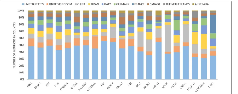
When considering the number of abstracts, the United States has published the greatest number of papers for each gene, except in one case (Fig. 10). For gene MYLIP,
China has more abstracts than United States, with 327 versus 312. Notably, there are some countries that follow closely behind the United States for some of the genes. For gene CEACAM3, the United States has 212 abstracts and Japan has 151. For gene CTSD, the United States has 145 abstracts, and France has 114.
However, when considering the effort put into each gene, the United States did not hold the largest propor-tion of effort (Fig. 11). Since the United States has pub-lished a lot of work on many genes, then the amount of effort for each gene decreases. For example, although the United States has published five times more papers than the United Kingdom on gene ESR1, the United Kingdom placed 20 % of its effort into gene ESR1, whereas the United States placed only 16 %. Information on country effort can be useful to find the priorities that each coun-try places on the genes, relative to other countries.
The MYLIP gene has seen more priority from China, with 5.0 % of China’s research effort into these gene, versus 0.2–1.2 % of effort coming from other countries
[image:12.595.58.542.89.448.2](Fig. 11). MYLIP also had more papers overall com-ing from China, rather than the United States, so this gene seems to be quite important for Chinese affiliated research. Although MYLIP does not appear to be a drug target, it seems to be upregulated by tamoxifen [31].
MYLIP codes for a myosin regulatory light chain (MRLC) interacting protein [32]. The MYLIP protein mediates ubiquitination, which is followed by degrada-tion of the MRLC. When the MRLC is degraded, then neurite (an axon or dendrite of a neuron) outgrowth is also inhibited.
Some other genes that received more interest and pri-ority from particular countries were ARL11 and 4.1 % of effort from Australia, CASP3 and 3.1 % of effort from China, BCL2L14 and 3.7 % of effort from The Nether-lands, CEACAM3 and 2.8 % of effort from Japan, and CTSD and 3.1 % effort from Italy (Fig. 11).
[image:13.595.58.552.89.286.2]An interesting point to consider is how regulated breast cancer research is in each country. If the direc-tion of breast cancer research is tightly regulated in some countries, then our study of publication effort towards the genes may reveal that direction. One way that the
Fig. 10 The proportion of gene mentions by each country
[image:13.595.58.541.141.546.2]Page 14 of 35 Jurca et al. BMC Res Notes (2016) 9:236
government of a country might regulate breast can-cer research is to encourage funding for groups which are studying particular genes. Promising genes to study might be the ones which have high potential for target drugs, or the ones that have a higher impact on breast cancer for that country’s population.
One limitation is that that our paper set may also include genes which have only been studied in mouse or rat models. Therefore, it may be difficult to confirm how these genes have a relationship to breast cancer in humans.
Which genes were never mentioned by the top 10 coun-tries? In total, there are 445 genes which were not men-tioned in any of the abstracts written by the top 10 coun-tries. The largest frequency of a gene not mentioned in the abstract of a top country is seven abstracts. Such a low frequency of seven, as compared to 18,913 for the ESR1 gene, indicates that the top 10 countries covered most genes. However, examining these genes may be interest-ing to to understand whether they have the possibility to be candidate genes or if they are outliers. To test this, we closely inspected some of genes, such as GLCE, which has abstract frequency of seven.
Gene GLCE codes for a protein called d-glucuronyl C5-epimerase, an enzyme which biosynthesizes the car-bohydrate portion of heparan sulphate proteoglycans (HSPGs) present on cell surface [33]. Enzymes which biosynthesize cell-surface sugar have the potential to be implicated in cancer growth because cell-surface sugar and proteins (proteoglycans) are involved in signal-ling to cells. Signalsignal-ling may indicate to a cell whether it should divide or not. If genes or proteins which have a role in such a signalling pathway are defected, then the cell may begin to divide infinitely, and therefore become cancerous.
Interestingly, in one of the few research articles that mentioned GLCE, it was shown to have an antiprolifer-ative effect on breast cancer cells. It was found that the down-regulation of GLCE may indeed lead to breast can-cer [33]. Therefore, the case study of GLCE shows that although some genes may not be mentioned as frequently as others in the abstracts, they still have potential to be important genes to breast cancer.
Another example is CHRM1 gene, which had a fre-quency of five abstracts. However, CHRM1 seems to be much involved in prostate cancer [34]. It codes for an acetylcholine receptor involved in the autonomous nerv-ous system. Again, cell-surface receptors have a high potential to be involved in cancer because they form a crucial part of cell signalling. CHRM1 has been shown to have an effect on prostate cancer in a high-impact arti-cle with 56 citations to date, although it was published
in 2013 [34]. Therefore, another reason that some genes may have a low mentioning in the abstracts is that they have been shown to be important in another cancer, yet researchers are only recently investigating their connec-tion to breast cancer. Genes which are not menconnec-tioned in many breast cancer abstracts may guide researchers to genes which require further investigation. With more research invested in these other genes, they may prove to be important biomarkers for breast cancer.
Hierarchical clustering
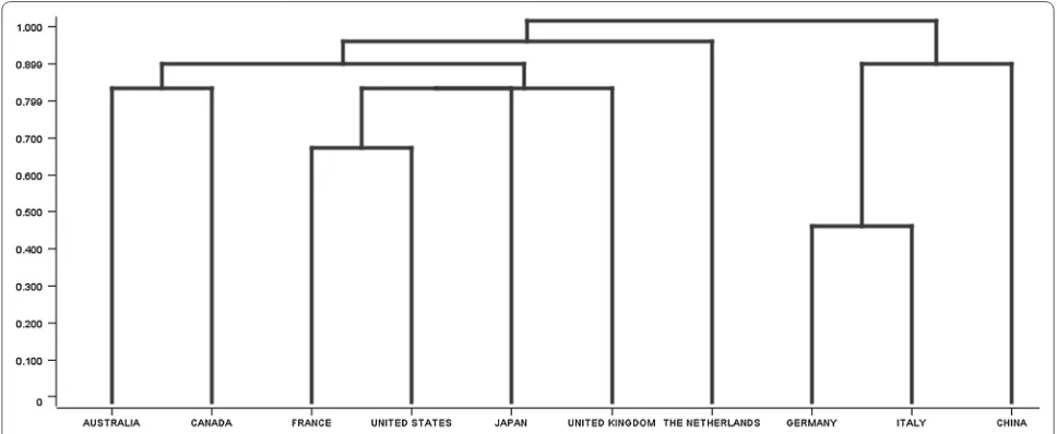
Hierarchical clustering is used to build a hierarchy of clusters, where two possible similarity measures that can be used are single-link and complete-link [8]. From a high-level perspective, Single-link clustering pro-duces clusters based on how similar the items are to one another, whereas complete-link clustering produces clus-ters based on how dissimilar the items are.
We applied hierarchical clustering between the coun-tries, based on the genes that each country studied. We used the complete-linkage measure, because this meas-ure has the advantage or producing more compact clus-ters, which leads to a clearer hierarchy. Our clusters were already very similar to each other, so we wanted to create more separateness. The results of the hierarchical clus-tering are displayed in Fig. 12. The hierarchical cluster-ing revealed that Germany, Italy, and China formed one branch, and then the second branch was formed United Kingdom, Japan, United States, France, Australia, and Canada. Lastly, a third branch was formed by the Nether-lands. A researcher can use Fig. 12 to see which countries have research interests in common.
Frequent pattern mining
Frequent pattern mining is used to find sets of items that occur frequently together in a database, and is often applied in grocery stores to discover which items the customers tend to purchase together [8]. Different algo-rithms such as apriori and FP-growth may be applied to generate frequent item sets from a collection of transac-tions. We applied the FP-growth algorithm to find the frequent item sets using the tool KNIME.
One measure of significance for item sets is support. Support is a decimal value that represents the proportion of transactions in the database that contain a particular item set. For example, if the item set A, B, C is found in 10 % of all transactions, then that item set has a support of 0.1.
an equal support value. For an additional explanation of maximal closed item sets, please refer to [8].
Genes frequently mentioned together by countries We computed the maximal closed frequent item set to find which genes are frequently mentioned together by each country. We arbitrarily considered the top five item sets and they are listed in Table 2. We then took a closer look at the item set which contained the following genes: BRCA1, ERBB2, ESR1. In Fig. 13, we used GeneMania to show that there is a relationship between the aforemen-tioned genes, as found in the gene expression data and the literature. Red edges represent physical interaction, and purple edges represent co-expression.
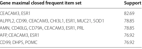
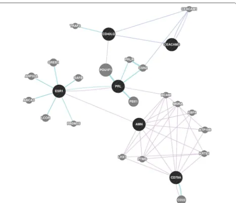
Genes frequently mentioned together every year Again, we computed the maximal closed frequent items sets for genes that are mentioned together every year. We arbi-trarily considered the top five item sets and they are listed in Table 3. We then took a closer look at the item set which contained the following genes: AMN, CD40LG, CD79A, CEACAM3, ESR1, PRL. In Fig. 14, we used GeneMania to show that there is a relationship between the aforemen-tioned genes, as found in the gene expression data and the literature. Blue edges represent co-localization, purple edges show co-expression, and turquoise lines show genes that belong to the same pathway.
The major genes related to top 10 diseases are repre-sented in Table 4. Related to this table more detailed analysis for each gene is listed in Appendix: Tables 9
and 10. These tables show more details about disease
associations for genes, studied country information, and genes that share more diseases with related genes.
Soft clustering
Soft clustering techniques are useful when items cannot be distinctly separated into clusters [8]. The clusters are formed such that each item has degrees of membership to the clusters. For example, item A may have a 0.1 mem-bership value to cluster X and a 0.7 membership value to cluster Y. This technique is often used when there are items that may belong to a ‘grey’ area. We used soft clus-tering techniques, such as fuzzy c-means, because the separation between the clusters was not very clear (see Fig. 16). Before deciding to use fuzzy c-means, we attempted to use density-based clustering techniques, yet they were unsuccessful and only returned one cluster. We used Matlab toolbox8 to perform fuzzy c-means (FCM) clustering.
[image:15.595.56.540.88.287.2]8 http://www.mathworks.com/matlabcentral/fileexchange/7486-clustering-toolbox (last visited 24 Nov 2014).
Table 2 Represented 5 highest maximal closed frequent item sets for Gene-Country
Gene maximal closed frequent item set Support
ERBB2, ESR1, PGR 48.43
EGF, ERBB2, ESR1 46.54
BRCA1, ERBB2, ESR1 45.91
BRCA1, BRCA2 45.28
CDKN2A, ESR1 45.28
[image:15.595.304.539.372.452.2]Page 16 of 35 Jurca et al. BMC Res Notes (2016) 9:236
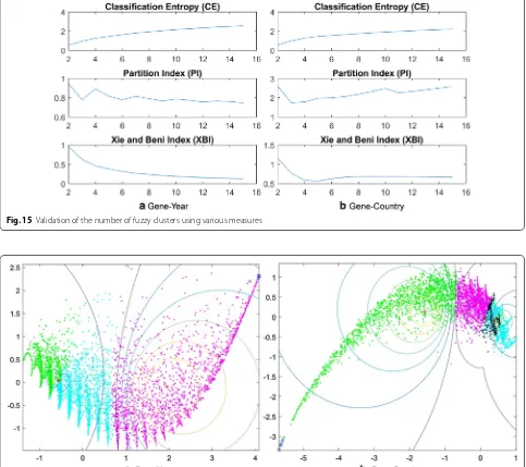
Finding the optimal number of clusters To find the optimal cluster number, we did cluster validation anal-ysis. No validation index is reliable only by itself, so that is why all the indexes c (cluster numbers) between 2 and 15 are shown in Fig. 15, and the optimum can be only detected with the comparison of all the results. We consider that partitions with less clusters are better, when the differences between the values of a validation index are minor. Cluster validation is used to evaluate how well the partitions have been produced [35], which is the reason why we chose the number of clusters as 3 and 4. For the cluster validation, we used four valida-tion indexes: partivalida-tion coefficient (PC), classificavalida-tion
entropy (CE), partition index (PI) and the Xie-Beni index (XBI).
In Fig. 15a, the main drawback of PC is that the values are monotonically decreasing as c increases. CE has the same problem: it monotonically increases as c increases, with a hardly detectable elbow point. Out of the scores for PC and CE, the number of clusters can be only rated to 3. More informative diagram is shown: PI sharply decreases at the c = 3 point. The XBI index is also mono-tonically decreasing and reaches the local minimum while c is increasing. Considering that PI is more useful, when comparing different validation indexes with the same c, we chose the optimal number of clusters as 3.
[image:16.595.56.537.84.367.2]In Fig. 15b, PC and CE again have the same problems: they are monotonically decreasing or increasing while c is increasing, which results in a hardly detectable elbow point. Out of the scores for PC and CE, the number of clusters can be only rated to 3. The more informative dia-gram is PI, which decreases at the c = 3 point. The XBI index also reaches its local minimum at c = 5. Consider-ing the PI and XBI indexes, we chose the optimal number of clusters as 4. To reduce the number of dimensions to 2 (from 159 for gene-country, and 52 for gene-year) we used Principal component analysis (PCA) through Mat-lab in order to visualize our data (See Fig. 16).
Table 3 Represented 5 highest maximal closed frequent item sets for Gene-Year
Gene maximal closed frequent item set Support
CEACAM3, ESR1 82.69
ALPPL2, CD99, CEACAM3, CHI3L1, ESR1, MUC21, SOD1 78.85 AMN, CD40LG, CD79A, CEACAM3, ESR1, PRL 78.85
AFP, CEACAM3, ESR1 76.92
[image:16.595.57.291.454.536.2]CD99, DHPS, POMC 76.92
Where do key genes lie in the soft clusters? We wanted to answer the following questions: Do key genes lie in the fuzzy areas of the clusters? Did the key genes belong among different clusters? Did all the key genes belong to one cluster? We wanted to compare the results of the fre-quent pattern mining to that of the soft clustering.
[image:17.595.61.538.83.495.2]The genes frequently mentioned together by country and year (see Tables 2, 3) which were found from a fre-quent mining analysis (FCM) are marked by a blue lxl in Fig. 16 which represents the soft clusters in 2D space. We then cross-matched the genes of the frequent pattern mining itemsets from Tables 2 and 3 with the genes of the FCM clusters. All of the genes were found to be in the fuzzy areas of the clusters, which means that none of the genes strictly belonged to one of the clusters (Fig. 16). This might mean that the genes in the closed maximal Table 4 Top 10 diseases associated with genes derived
from the union of the top 5 gene-year and gene-country itemsets
Disease name Genes
Breast neoplasms ERBB2, ESR1, PGR, EGF, BRCA1, BRCA2, CD99, AFP
Adenocarcinoma ERBB2, PGR, EGF, CDKN2A, CD99 Mammary neoplasms, experimental ERBB2, PGR, BRCA1, AFP Carcinoma ESR1, PGR, BRCA1, CD99 Prostatic neoplasms ERBB2, EGF, BRCA1, BRCA2 malignant neoplasm breast PGR, BRCA1, BRCA2
Glioma ERBB2, CDKN2A, CHI3L1
Hypertension CHI3L1, SOD1, POMC
Neoplasm BRCA1, CDKN2A, CD99
Ovarian neoplasms ERBB2, BRCA1, BRCA2
Page 18 of 35 Jurca et al. BMC Res Notes (2016) 9:236
frequent item sets are key genes that are often mentioned with other genes as well across articles.
Network analysis
Network analysis, often called “Social Network Analysis” because it was first developed to study social structures,
[image:18.595.59.538.88.362.2]is a strategy to find communities within data [9]. Net-work analysis takes into consideration a set of “actors” and a set of “actions” between the actors. The character-istics of the actors are secondary in importance to the relationships between the actors.
[image:18.595.57.540.154.583.2]Fig. 15 Validation of the number of fuzzy clusters using various measures
There are various measures that one can use to find key actors within the network. One measure is called modularity, which is an integer that denotes what com-munity a particular actor belongs to. Another measure is called closeness, which is a relative measure for the num-ber of shortest paths an actor has to all other actors. The higher the closeness value that an actor has, the more connected this actor is to all other actors through short paths. In terms of sociology, an actor with a high close-ness would be highly efficient at spreading information to a lot of people. A third measure that we will reference in our work is betweenness. Betweenness measures the number of shortest paths that pass through an actor. In terms of sociology, an actor with high betweenness is the best “middle man”, and if removed from the network, will disconnect a lot of people and communities.
We applied network analysis on the genes that we collected by considering the genes as “actors”, and the “actions” as co-occurrences within the abstracts. To con-duct network analysis, we first built a weighted adjacency matrix between all of the genes we collected, such that each intersected value between two genes represented the number of abstracts that these two genes co-occurred within.
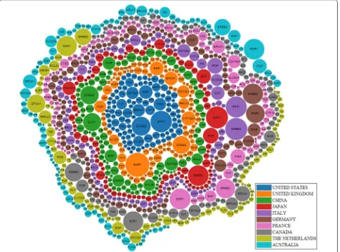
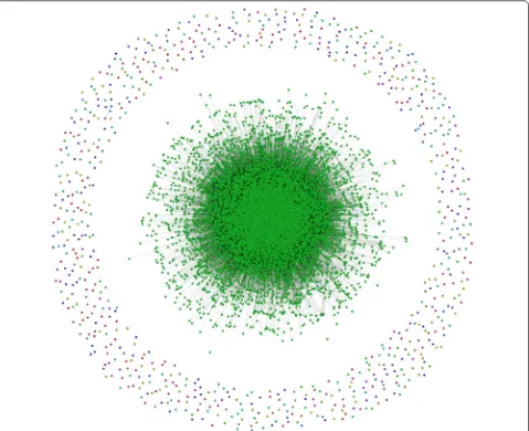
[image:19.595.60.539.306.696.2]After creating the gene–gene network from the adja-cency matrix, the network contained noise comprised of some genes which were unconnected to any other genes which made it difficult to comprehend, as seen in Fig. 17. The full network contained 8400 nodes with 213,894 edges (Table 5). To get more concise results, we then did connected component analysis in order to reduce the number of edges and nodes to get the giant component.
Page 20 of 35 Jurca et al. BMC Res Notes (2016) 9:236
If the largest component takes a significant part of the graph, then it can be considered as the giant component [36]. Our giant component contained 90.71 % of the full network (see Table 5). However, the number of edges in the giant component, 213,877 was almost unchanged from the number of edges in the full network.
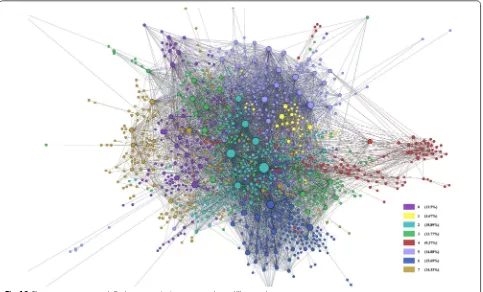
To further prepare the network for analysis, we pruned edges with weight less than 10, where edge weight is the frequency of genes’ co-occurrence in the abstracts. The pruned network was therefore more condensed and showed stronger connections, or the heart of the full network 18. To the pruned network, we applied some network measurement techniques: closeness, between-ness, and modularity. The results of the measurement are reported in Table 6, ordered by their closeness and betweenness values. Depending on these measurements, we can see the first 10 most important genes in the net-work, which are listed in Table 6.
In Table 6, the modularity values show which genes are making communities together, similar to clustering. For example, ESR1, ERBB2, SLC20A2, EGF, and PGR are part of the same community because they all have a modular-ity class of 2. To validate these results, we wanted to see if this community could also be found in experimental data. We manually validated the genes listed in Table 6
using BioGrid which is similar to GeneMania, because it
uses analyzed experimental data from published articles in order to show communities of genes. We found that all genes except SLC20A2 had a physical interaction in the community. However, when we entered ESR1, ERBB2, SLC20A2, EGF, and PGR into GeneMania, it showed that all genes were indirectly related, either through shared protein domains, co-expression, pathways, etc. We, therefore, found some experimental evidence that genes in group 2 were indeed related, although the interaction may be indirect. Researchers can use these communi-ties to find genes which may be indirectly connected, and then use experimental evidence to potentially strengthen the connection of these genes into the community.
Similarly, for genes CDKN2A, BRCA1, and HLA-H which all belong to modularity class 6, we performed analysis similar to that of modularity class 2. Using BioGRID, we found published evidence that CDKN2A and BRCA1 have a direct physical interaction, but not with HLA-H. However, using GeneMania, we found that there is an indirect interaction between HLA-H and the other two genes. For CDH1, we performed a different analysis, to confirm that this gene has a strong gene-dis-ease relationship with breast cancer. We found that CDH1 has been experimentally shown to strongly influ-ence the presinflu-ence of breast cancer.9 For ACAD-9, we per-formed analysis similar to that of CDH1. To the best of our knowledge, we could not find experimental data which linked ACAD-9 to breast cancer. However, we decided to look further down the list of the most con-nected genes to find the next two genes which belong to class 5, so that we could perform an analysis similar to class 2 and 6. The next two well-connected genes of class 5 are MAPK10 and KRAS. GeneMania indicated that these genes are indirectly connected. Since MAPK10 codes for a protein centrally involved in a host of signal-ling pathways,10 it is likely that it is involved in cancer. Signalling proteins indicate to the cells whether they should proliferate or not, so should the protein function be defected, the cell may divide indefinitely as a cancer [34].
We examined the smallest community (community 1 is chosen, yellow nodes in Fig. 18, which includes 229 nodes) from the pruned network to see how well the gene nodes were connected using the GeneMania resource. The results of the analysis are displayed in Fig. 19, where all genes are connected through co-expression, except for four genes: SPRR2A, C5orf27, FOXP4, and MT-ND3. The large number of connections through co-expres-sion provides experimental support for this community. Genes which were not co-expressed with the others in
9 http://ghr.nlm.nih.gov/gene/CDH1 (last visited 24 Nov 2014). 10http://www.ncbi.nlm.nih.gov/gene/5602 (last visited 24 Nov 2014).
Table 5 Statistical information for gene–gene network
Nodes % Edges %
Full network 8400 100 213,894 100
Giant component 7620 90.71 213,877 99.99 Pruned giant component 1089 12.96 6815 3.19
Table 6 Network Analysis measurements for the gene– gene network
The top 10 genes with the highest betweenness are shown, as well as the top 10 genes with the highest closeness. The modularity class is also shown, where it denotes the community that the gene belongs to
Between-ness centrality
Modularity
class Closeness centrality Modularity class
ESR1 0.09 2 ESR1 0.62 2
ERBB2 0.06 2 ERBB2 0.6 2
CDKN2A 0.04 6 CDKN2A 0.58 6
SLC20A2 0.03 2 SLC20A2 0.57 2
EGF 0.02 2 EGF 0.57 2
PGR 0.02 2 PGR 0.56 2
BRCA1 0.02 6 ACAD9 0.55 5
CDH1 0.02 0 CDH1 0.55 0
ACAD9 0.02 5 MAPK10 0.55 5
the community may be genes which have yet to be vali-dated into the community; this community may serve as a hint to primary researchers who wish to find other con-nections for these genes. If a researcher would like to fur-ther validate the ofur-ther communities with GeneMania, we have provided the full list of network analysis genes and their modularity class (the community they belong to) in Additional file 1.
Table 7 shows which diseases are more common in each community so that we can group and target these communities based on their problem to cure. More detailed information about community-disease relation is represented in Appendix: Table 8. This table shows the top five diseases for each community and the num-ber of genes related to each disease and the name of these genes. For example, communities 0, 2, 3, 4, and 6 are more related with cancer and its types such as breast cancer. While these communities are targeted for can-cer treatment, communities 1 and 4 for diabetes mel-litus, and community 7 for leukemia may be focused on treatment.
Castro et al. [37] have reported in their work that ESR1, FOXA1, GATA3, SPDEF, AR, RARA and XBP1 are criti-cal for ER+ disease and known to be central to breast
cancer risk. In our results, all these genes are found in community 2 which is the mainly related to the breast
cancer, except that XBP1 is in community 3 (see Addi-tional file 1).
Conclusions
The work described in this paper contributes a novel framework which is capable of investigating how research groups in various countries address breast can-cer. We investigated the genes or proteins studied by vari-ous research groups by carefully analyze their published research articles to identify the molecules they reported as biological biomarkers of breast cancer. Interestingly, we realized that researchers have reported interest in a variety of genes over time and even based on the coun-try where the research is conducted. This might be due to other external factors particular and specific to each community or country, though some of the discovered genes were reported to have similar function. Thus we demonstrated how the gene–gene, year, and gene-country relationships provide some interesting gene hypotheses that primary researchers might consider in their research. Further, this paper shows the power of integrating data mining and network analysis techniques.
[image:21.595.58.541.88.380.2]As future work, we will also account for the seman-tic relations or directionality between the genes. For example, we will find relationships such as “gene A up-regulates gene B”, rather than “gene A and gene B have a
Page 22 of 35 Jurca et al. BMC Res Notes (2016) 9:236
relationship due to co-occurence within an abstract”. We will also attempt to upgrade the text mining application to perform full-text analysis, rather than abstract analy-sis. Although abstracts are useful because they summa-rize the articles, the full text of the articles contain more
information, especially the experimental analysis and discussion sections. However, full-text mining presents many more challenges, such as errors from conversion to plain text, and problems with reading text from tables and figures [38]. We are currently investigating other Table 7 Common diseases in each community
Cancer Breast
cancer Prostate cancer Diabetes mellitus Colon cancer Obesity Leukemia Hyperten-sion Athero-sclerosis Rheu-matoid arthritis
Embryoma
Community 0 X X X X X
Community 1 X X X X X
Community 2 X X X X X
Community 3 X X X X X
Community 4 X X X X X
Community 5 X X X X X
Community 6 X X X X X
Community 7 X X X X X
[image:22.595.59.538.86.446.2]types of cancer and diseases in general. We expect to report some interesting finding shortly.
Authors’ contributions
GJ helped in developing the methodology, in running the tests and in analyz-ing the results. OA helped in developanalyz-ing the methodology, in crawlanalyz-ing the data and in running the tests. AA helped in the design of the study, in drawing the figures and in the analysis of the results. SG participated in integrating the various processes to produce the integrated framework, and in the analysis. TO helped in crawling the data and in developing the methodology. DD helped in Additional file
Additional file 1. Additional Tables.
the analysis and validation of the results. RA participated in the development of the methodology and in the analysis of the results. GJ, OA, AA and RA drafted the manuscript. All authors read and approved the final manuscript.
Author details
1 Department of Computer Science, University of Calgary, Calgary, AB, Canada. 2 College of Computer Science and Technology, Jilin University, Changchun, China. 3 Department of Computer Engineering, TOBB University, Ankara, Turkey. 4 Departments of Pathology, Oncology and Biochemistry & Molecular Biology, University of Calgary, Calgary, AB, Canada. 5 Department of Computer Science, Global University, Beirut, Lebanon.
Competing interests
The authors declare that they have no competing interests.
Appendix
See Tables 8, 9, 10 and 11. Table 8 Gene-disease associations from gene–gene analysis
Community
ID Disease names # of total genes in community
# of genes sharing disease
Gene names
0 Cancer 2105 133 EPHB4, MYCN, SOX9, RPL22, SPARC, ABL1, EAF2, PDGFA, PDGFB, SLC39A1, SPP1, RPS3, UNC5B, PIWIL1, GALR2, ETS1, DAG1, ETV4, EWSR1, CHD4, ITGA3, F2R, MMP20, ITGAV, ADAM10, ITGB3, ITGB4, TUBA4A, ZEB2, PTHLH, PTH1R, NMU, TWIST1, STRAP, JAG2, S100A4, HOXA9, BMI1, GJA1, BMP2, BMP4, BMP7, JUP, BMPR1A, JTB, CD82, HOXC8, GPC3, RHOU, NUAK1, CTNNBIP1, ITIH1, BSG, YAP1, GLI1, CTAGE1, PVRL1, KIF14, PLAU, ALAS1, MMP1, MMP2, MMP7, MMP9, MMP11, MMP14, SDC1, NANOS1, ARHGEF6, KIF11, VGF, KLK11, NID2, SFRP1, SFRP2, SFRP4, CD248, ADAMTS1, PODXL, ANXA1, USP28, WNT1, WNT2, WISP1, WNT5A, WNT7A, ARL6IP5, SLIT2, WNT2B, RIN1, SHH, GEMIN5, LAMC2, MMP26, HIF3A, RUNX2, RUNX3, KLK3, CLDN2, CLDN1, SLC2A4, ARPC2, POSTN, USP6, ORM2, HHIP, SMURF2, EFNB2, SPINT2, CD9, FAM107A, CYR61, TIMP2, TIMP3, YKT6, SNAI2, SP5, ROBO1, IRAK3, NDC80, SNAI1, CTNNB1, LUM, CTSB, KLK13, PCDH8, BCR, DKK3, RPL10, SMAD2, SMAD4, RGL4, SMAD7
Breast cancer 65 HOXA5, WISP3, WISP2, MEST, PTPN1, HOXB13, BMP5, BMP6, UBE2B, TLK1, ETV1, KLK4, NMI, NEUROD1, ADAM28, CSF1R, PER2, RHOU, LIMD1, PTPRJ, TIMP1, ARNT2, ARID4A, TIMP4, INHBA, LATS2, TNC, USP28, SLC2A3, IGHMBP2, IBSP, VCAN, VTN, AFF3, WASF2, SERPINE1, CST3, POLI, ETS2, CSTA, LAMA3, CTGF, ADAMTS8, FURIN, MMP3, MMP8, LCN2, SIX1, MMP13, WNT9A, PCBP1, F2RL1, F3, CTSK, F7, TUBA4A, F10, SERPINA5, SDC4, RNF11, BMPR2, ANXA8L2, KLK2, PINK1, HOXA1
Prostate
cancer 63 AMBP, RNF14, KLK4, KIAA0196, PTPN1, BMP5, BMP6, BMPR1B, BMPR2, PTPN12, HOXC8, CSF1R, PDX1, EAF2, SERPINA5, PAGE4, SPINT1, SLC39A1, ACAT2, PLG, DSPP, GLI2, COPE, IBSP, VCAN, CLPTM1, EHF, SERPINE1, DVL1, ETV1, PDGFD, LATS2, CDCP1, PLAU, CRISP3, DAZL, TREX2, ELK4, TIMP1, TSPY1, RLN2, ACVR2A, CYSLTR1, ITGA7, MMP12, KLK3, MMP15, MMP17, F2RL1, ATP2A1, F3, CTSK, INHA, GFI1, HOXB13, TIMP4, RPL10, KLK2, ADAMTS9, CST3, RLN1, ZNFX1, ADAMTS13
Diabetes
mellitus 60 RLN2, XYLT2, SERPINB2, PKLR, GJA1, BMP4, BMP6, BMP7, GREM1, NEUROD1, FBP1, UTS2, CALD1, TIMP1, HLA-DMB, TIMP3, PTPRN2, SPP1, TJP1, TNC, PTX3, KCNJ10, PLA2G4A, CLPS, SERPINE1, CST3, CD9, MTTP, SHH, LRP5, ANKRD1, PTPN22, KIF11, CTGF, MMP14, GCK, ISL1, MMP1, MMP2, FTO, MMP8, TIMP2, DCN, F2, CTSB, AKR1B1, F3, ITGB3, CLOCK, AQP7, SDC2, PTGES2, SLC2A4, GGT1, FABP1, FABP2, PINK1, CYBA, SMAD7, FOXC2
Colon cancer 51 PMP22, MMP25, RNF14, HSPE1, PTPN1, C1GALT1C1, BMPR1A, DKK4, HTR2A, CYSLTR1, STRAP, TIMP1, TIMP4, LLGL1, TJP1, TNC, ASCL2, KLF9, FDPS, TOMM34, CNOT7, ZKSCAN3, SER- PINE1, CEACAM7, SOX17, OLFM4, LYPD3, PLA2G4A, HRH2, DLL1, NTN1, ADAMTS13, MMP3, ACVR2A, LCN2, MMP10, CDCP1, MMP13, ADAMTSL3, SRPRB, F2RL1, AKR1B1, CTSH, CLDN12, ITGB6, SDC2, KLK1, GGT1, B3GNT8, CD226, ACTR2
1 Diabetes
mellitus 229 29 GH1, GHR, SOCS2, NAMPT, LIPE, RETN, IGF2R, IGFBP1, IGFBP3, NUDT1, LNPEP, ADIPOR2, INS, FGF21, LPL, RBP4, POMC, APOA1, APOA2, IRS1, IDE, APOC3, HSD11B1, CFI, PLTP, LEPR, SLC2A2, ADD1, FABP4
Obesity 23 GH1, GHSR, LIPE, IGF1, IGF2, IGFBP3, IGFBP6, ADIPOR2, INSR, SOCS3, SHBG, POMC, APOA2, IRS1, HSD11B1, RETN, SERPINA6, LEP, LEPR, SLC2A2, RBP4, FABP4, ADRB1
[image:23.595.54.538.275.716.2]