A numerical flow simulation of a mixed flow pump

A NUMERICAL FLOW SIMULATION OF A MIXED-FLOW

PUMP

M T Stickland, T J Scanlon

University of Strathclyde, Department of Mechanical Engineering Glasgow, G1 1XJ Scotland

[email protected] J Fernández

Universidad de Extremadura, Dpto. de Electrónica e Ingeniería Electromecánica Avda. de Elvas s/n. 06071 Badajoz, Spain

[email protected] E Blanco, J Parrondo

Universidad de Oviedo, Área de Mecánica de Fluidos Campus de Viesques, 33271-Gijón (Asturias), Spain

[email protected]

Abstract

This paper presents a comparison between the experimental data available on the velocity

field for a mixed-flow pump (non-dimensional specific velocity of 1.52) and the predictions obtained from computations with a general-purpose CFD code, Fluent 5.3. Particular attention was paid to the prediction of the turbulence components, when using a Reynolds Stress

turbulence model. Calculations were performed for the design flow-rate and for off-design conditions. Whereas the prediction of the overall pump head agrees adequately with the

measurements, the prediction of the turbulent component of the axial velocity appears to be systematically small.

keywords

Nomenclature

r impeller radius

ut tangential velocity

v’z turbulent component of axial velocity

wu tangential relative velocity

x peripheral coordinate z axial coordinate

β tangential angle

φ flow coefficient

1. INTRODUCTION

During the last decade there has been a progressive increase in the use of commercial CFD software to model the flow through turbomachinery. In many cases, the general characteristics

of the flow, for instance the head-flow rate performance curve for centrifugal machinery, may be predicted quite satisfactorily, in spite of not using a very large number of discretization

cells and imposing uniform flow boundary conditions very close to the inlet and outlet of the machine [1,2]. Following this line of work, this paper presents an investigation on the ability of one such commercial code, Fluent 5.3, to predict the flow behaviour through a mixed-flow

pump (non-dimensional specific speed of 1.52) with a single rotor-stator stage; the study considered not only the overall performance characteristics of the pump, but also some

Laser Doppler Anemometry (LDA) measurements in the rotor, the stator and in the

intermediate regions, for a number of air flow-rates through the pump. In particular the spatial distributions of several components of the velocity were obtained as well as the turbulent

component of the velocity in the axial direction.

This paper presents the discretized model developed for that pump and the predictions

obtained by means of the Fluent 5.3 code for 3-dimensional unsteady flow. The results obtained for two flow-rates, 45.6% and 100% of the design flow-rate, using three different

turbulence models; standard k- , RNG (re-normalisation group) and Reynolds Stress, are compared to the experimental set of data in order to evaluate their potential for the analysis of such flows.

2. TEST PUMP

Figure 1 shows a sectional view of the test pump. It was a mixed flow bowl type machine, with five impeller blades mounted on a conical hub, and nine stator blades in a diffuser to

return the diagonally outward flow back to the axial direction. Main blade impeller and stator dimensions are summarised in Table 1. The casing was fitted with a large transparent window

that gave optical access to the flow passages through the pump from the impeller inlet to the stator outlet. The velocity at some given axial and radial position could be measured by means of a 2D LDA system coupled to a data acquisition system which used a shaft encoder to relate

the individual velocity measurements to the rotating frame of reference. Full details of the pump geometry and dimensions, as well as details of the measuring system with assessment

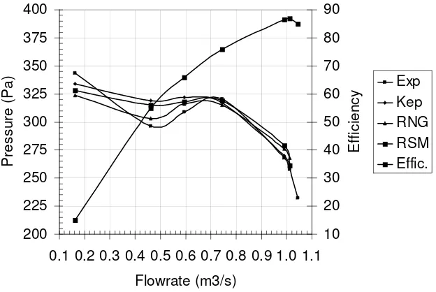
indicated a maximum efficiency of 87% for a flow-rate of 1.010 m3/s and a total pressure rise

of 250 N/m2 (flow coefficient of 0.344 and head coefficient of 0.280). The corresponding non-dimensional specific velocity was 1.52.

Figure 1: Cross-section of the test pump.

Impeller Stator

r (mm) z (mm) β (deg) r (mm) z (mm) β (deg)

Inlet, hub 90.7 776.1 37.0 188.9 995.5 59.0

Inlet, tip 210.9 750.0 28.6 261.6 1017.8 53.0

Outlet, hub 177.8 913.7 46.1 91.2 1247.5 0.0

Outlet, tip 251.9 879.0 26.7 209.9 1279.6 0.0

r = radius, z = axial coordinate, β = tangential angle

Figure 2: Performance characteristics of the test pump.

The experimental results obtained on the velocity distributions throughout the pump for a number of flow-rates are given in Carey et al. [4] for the impeller region, Carey et al. [5] for

the intermediate region between the impeller and stator and Carey et al. [6] for the stator region. These sets of data include the turbulent component of the axial velocity (the other turbulent components could not be obtained from the LDA data collected). Experimental

uncertainty for the velocity data was established at less than ±5%.

3. MODEL AND COMPUTATIONAL METHOD

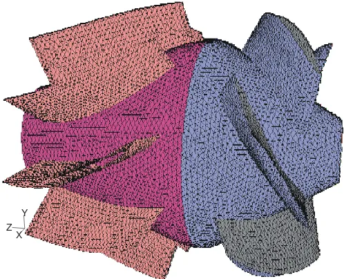
To perform the numerical calculations, an unstructured mesh was generated throughout the pump, from the inlet bell-mouth to the exit of the stator blades. A total of 2.5x105 cells were

considered for the rotor region, and 2.5x105 cells for the stator and intermediate regions. Figure 3 shows a general view of the mesh on the surface of the hub and the blades of both the rotor and stator. Such a large number of cells is not sufficient for a precise simulation of

200 225 250 275 300 325 350 375 400

the boundary layer zones. The extremely fine mesh that such calculation would require in the

near-wall regions was far beyond the capabilities of the computational equipment used. However, according to previous experience with other machines, the mesh was adequate to

model correctly the general flow phenomena and the overall performance.

Calculations were performed with the commercial code Fluent 5.3, which is capable of

handling unstructured grids with relative displacement between regions in time. This code solved the incompressible 3-dimensional Navier-Sokes equations including the centrifugal

and Coriolis forces source in the impeller and the unsteady flow terms. Three different

turbulence models were used: a standard k-ε, RNG and Reynolds Stresses. Since the grid size

was not fine enough for the calculation of flow in the boundary layers, conventional wall functions, based on the logarithmic law, were imposed. In the differential equations, upwind

second order discretizations were used for the convection terms, and central difference schemes for the diffusion terms. During the iteration process the pressure-velocity coupling

was achieved by means of the SIMPLEC procedure.

Figure 3: Detail of the mesh on the hub and blades surfaces on rotor and stator.

Z Y

As a boundary condition, the flow at the inlet of the pump was assumed to be steady, with

uniform velocity in the axial direction. The value of the inlet velocity determined the circulating flow-rate considered. This flow-rate was either the design flow-rate (flow

coefficient φ=0.344) or 45.6% of the design flow-rate (φ=0.157). At the outlet of the pump the

condition imposed was constant static pressure. On the solid walls the non-slip condition was imposed. At the interfaces between regions with relative motion, i.e. at the inlet-rotor

interface and at the rotor-stator interface, the coupling of the fluxes across the grid interfaces had to be re-determined at each new time step.

The time step used during the unsteady calculations was 0.004775 seconds. With this time-step, a complete revolution was obtained after 100 steps (one blade passage every 20 steps). The number of iterations was adjusted to reduce the residuals below an acceptable value for

each time step. In particular, the ratio between the sum of the residuals and the sum of the fluxes for any given variable in all the cells had to be less than 10-5. The initial conditions

applied were those for a steady state calculation. When these results were used as the initial conditions for the transient solution around seven impeller rotations were necessary in order for the solution to achieve full transient status.

The numerical grid was divided into 5 separate regions in order to process them on a parallel

Head coefficient

Flow coefficient

Experiment

Model:

k-ε

Model:

RNG

Model:

Re stresses

0.157 0.332 0.357 0.339 0.353

0.344 0.280 0.293 0.300 0.292

Table 2: Measurement and prediction of pump head

4. PREDICTION OF THE PUMP HEAD

An initial series of calculations were conducted to check the independence of the general results of the model on the mesh size and numerical time step. For each turbulence model used, it was found that, either multiplying or dividing by two both the grid size and the time

step, resulted in variations in the pump head predictions of less than 1%. Table 2 (see also Figure 2) compares the calculated values of the head of the pump with each of the three

different turbulence models, for the best efficiency flow-rate (φ=0.280) and for off-design

conditions (φ=0.157). The head predicted by the three models were greater than the

experimental, i.e. apparently the numerical simulations produce an optimistic estimate of the internal losses. Nevertheless, differences were always less than 7.5%, which may be

considered an acceptable result given the complexity of the pump under simulation. The

predictions of the standard k-ε model and the Reynolds stresses model were remarkably

4. NUMERICAL RESULTS

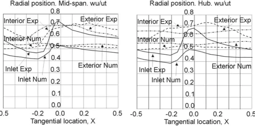
Figure 4 presents the results obtained for the tangential component of the relative velocity, wu,

in the intermediate region between the impeller and stator for 45.6% of the design flow-rate. This relative velocity was obtained by subtracting the tangential velocity of the impeller blade (at the corresponding radial position) from the absolute velocity, i.e. it is expressed in terms of

the relative frame of reference. Each of the diagrams in Figure 4 corresponds to one radial position (hub, tip or mid-span), and present the velocity variation along the peripheral

direction for a length equivalent to one impeller channel width. This peripheral direction is denoted as the co-ordinate x; the value x=0 indicates the position of the outlet edge of a blade of the rotor, whereas x=1 corresponds to the height of each channel in the impeller. Each of

the diagrams contains 6 curves: the predictions from the Reynolds stress turbulence model plus the experimental data, for three different axial positions: inlet, interior, and outlet. The

velocity values have been normalised by the tangential velocity ut on the rotor hub at middle

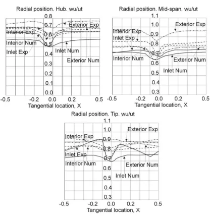
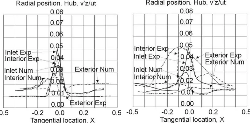
axial position (ut=27 m/s). Figure 5 presents the values obtained for the turbulent component

of the axial velocity, vz’, under the same conditions of Figure 4. Figures 6 and 7 present the

results corresponding to 100% of the best-efficiency flow-rate.

In general, for both flow-rates, the results obtained regarding the relative velocity wu show

similar values to the experimental data: usually the differences were within 15% of the measured values. However the errors for the turbulent component vz’ were significantly larger

(up to 50%), especially when increasing the distance from the outlet of the impeller. In general the turbulence levels predicted were excessively small, though similar trends can be

It may be deduced that the use of this simulation model for the pump tested may be

considered adequate for the prediction of global pump characteristics and, also, it is helpful in describing some flow details such as the rotation of the flow though the intermediate region

between rotor and stator. However the model appears to be inadequate for the prediction of the turbulence features.

Figure 4: Distribution of the tangential relative velocity, wu, in the intermediate region

Figure 5: Distribution of the turbulent component of the axial velocity, vz’, in the intermediate

Figure 6: Distribution of the tangential relative velocity, wu, in the intermediate region

Figure 7: Distribution of the turbulent component of the axial velocity, vz’, in the intermediate

5. CONCLUSIONS

A study has been conducted to check the applicability of a commercial CFD code, Fluent 5.3,

to predict the flow characteristics, including turbulence levels, for a mixed flow-pump operating under some given value of flow-rate. Two flow-rates and three different turbulence models were considered. Theoretical predictions were compared to an exhaustive set of

experimental data available for a particular pump. The results obtained indicate that, when conducting the calculations on a computer with standard processing capabilities, the

predictions regarding the overall performance of the pump (i.e. the pump head) overestimated the measured values; maximum errors were less than 7.5 % which may be considered acceptable. However, larger errors were observed regarding the prediction of the tangential

component of the velocity in the intermediate region between rotor and stator, when using a Reynolds Stress model in the computations. Finally, the predictions of the turbulence

component of the axial velocity showed trends similar to those of the experimental data, but the calculated values were usually up to 50 % smaller. These results suggest that improvement in the prediction of the turbulence features of the flow through turbomachinery,

based on commercial general-purpose CDF codes, requires a much smaller grid size than the one used for the present study.

ACKNOWLEDGEMENTS

The authors gratefully acknowledge the financial support of the Ministerio de Ciencia y

REFERENCES

1. Blanco E., Fernández J., González J. and Santolaria C.. Numerical flow simulation in a

centrifugal pump with impeller-volute interaction. ASME 2000 Fluids Engineering Division Summer Meeting, Boston (USA), paper FEDSM200-11297 , 2000.

2. Shi F. and Tsukamoto H.. Numerical Study of Pressure Fluctuations Caused by Impeller-Diffuser Interaction in a Impeller-Diffuser Pump Stage. ASME Journal of Fluids Engineering 123,

466-474, 2001.

3. Carey C., Fraser S.M., Rachman D. and Wilson G.. Studies of the flow of air in a model

mixed-flow pump by laser Doppler anemometry. Part 1: Research facility and

instrumentation. NEL Report nº 698. East Kilbride, Glasgow (U.K.): National Engineering

Laboratory, 1985.

4. Carey C., Fraser S.M., Rachman D. and Wilson G. Studies of the flow of air in a model

mixed-flow pump by laser Doppler anemometry. Part 2: Velocity measurements within the

impeller. NEL Report nº 699. East Kilbride, Glasgow (U.K.): National Engineering

Laboratory, 1985.

5. Carey C., Fraser S.M., Rachman D. and Wilson G. Studies of the flow of air in a model

mixed-flow pump by laser Doppler anemometry. Part 3: Velocity measurements between

rotor and stator blade rows. NEL Report nº 707. East Kilbride, Glasgow (U.K.): National

6. Carey C., Fraser S.M., Shamolahi S. and McEwen D. Studies of the flow of air in a model

mixed-flow pump by laser Doppler anemometry. Part 4: Velocity measurements within the

stator/diffuser. NEL Report nº 714. East Kilbride, Glasgow (U.K.): National Engineering

Laboratory, 1989.

LIST OF FIGURES

Figure 1: Cross-section of the test pump.

Figure 2: Performance characteristics of the test pump.

Figure 3: Detail of the mesh on the hub and blades surfaces on rotor and stator.

Figure 4: Distribution of the tangential relative velocity, wu, in the intermediate region

between impeller and stator (45.6% of the design flow-rate).

Figure 5: Distribution of the turbulent component of the axial velocity, vz’, in the intermediate

region between impeller and stator (45.6% of the design flow-rate).

Figure 6: Distribution of the tangential relative velocity, wu, in the intermediate region

between impeller and stator (design flow-rate).

Figure 7: Distribution of the turbulent component of the axial velocity, vz’, in the intermediate

region between impeller and stator (design flow-rate).

LIST OF TABLES