Control of Variable Speed Variable Pitch Wind Turbines using Mpc and Qft

International Journal of Innovative Technology and Exploring Engineering (IJITEE) ISSN: 2278-3075, Volume-8 Issue-12, October 2019

Control of Variable-Speed Variable-Pitch Wind

Turbines using Mpc and Qft

Y. Bharathi Devi, P. Bharat Kumar, P. Sujatha

Abstract: Tracing of operating point where maximum power is extracted, regulation of power and speed are the major control objectives for the main component of WECS i.e., wind turbine. A controller with objective designed for one operating region may not sustain better performance in any other operating region. To overcome such issues and achieve improved nature of performance in any operating region using a new advancement in controller with future prediction capability and thus attain the required control objectives. In this work, such objectives are achieved by using continuous-time multi model predictive control and Quantitative Feedback Theory control (QFT). Both the controllers’ performance is compared using simulink studies for a wind turbine model. Simulation results will show the performance of the above mentioned control scheme. The entire simulation work will be carried out on MATLAB/Simulink environment.

I. INTRODUCTION

The best type of renewable source available in the present scenario is the wind. Wind Energy conversion systems (WECS) can be utilised for the conversion of kinetic energy of the wind to the mechanical energy. Wind pump, windmill and the present day wind turbine are examples of WECS. Wind power is utilised to propel boats, grind grain, and also to pump water which can be known from previous history. Using new ways of wind energy gradually spread throughout the world, wind mills and pumps are widely used for food production by the people of middle-east during the 11th century. Large Wind pumps are first developed by Dutch people. Of the total electricity generation of India, nearly 4% is through Wind Power, which accounts for almost 10% of the India’s overall installed capacity of power generation. Across different states of India, there is a large increment in the number of wind energy installations. Wind energy has many significant favourable features. Among them the important ones include unlimited, free, renewable resource. It’s a fuel source which doesn’t pollute the air and also there will be no atmospheric emissions from Wind Turbines, but these turbines are a great threat to wildlife such as bats and birds. Deforestation creates an impact on environment and also creates Noise Pollution. In spite of few disadvantages also, much interest is being shifted to renewable energy sources. As the environmental concerns are increasing in present days, many countries are assisting much to the clean energy research and thus lead to the improvement of power generation from the wind. By the reach of 31 March 2019, the overall installed capacity of wind power was 36.625 GW. India targeted to accomplish 60 GW of electrical energy from wind by the end of 2022.

Revised Manuscript Received on October 05, 2019

Y. Bharathi Devi, M. Tech (student), Dept of Electrical Engineering, JNTUA, Anantapur, AP, India.

P. Bharat Kumar, Lecturer, Dept of Electrical Engineering, JNTUA, Anantapur, AP, India.

P. Sujatha, Professor, Dept of Electrical Engineering, JNTUA, Anantapur, AP, India.

The various components that constitute the WECS are wind turbine, generators, storage and grid [1]. Among these, the key component is the wind turbine. These devices can be widely categorised based on their axis alignment into two types: Horizontal (HAWT) and vertical (VAWT) axis wind turbines. The most usually used type is Horizontal Axis type of Wind Turbine as it has greater energy conversion efficiency because of its blade design though it needs stronger tower support because of more weight of nacelle and also cost of installation is more related to VAWT. Both onshore and offshore nature of models also exists. Mostly, in domestic and private areas where the energy demand is less we use VAWT. Extraction of maximum power, speed and power regulation are the major control objectives for a wind turbine. The control strategies in wind turbine literature depend on the objective in the present operating zone of the wind turbine. Maximum Power Point Tracing is the phenomenon used mostly with wind and solar type of systems to maximize extraction of power in all conditions. MPPT is the process of extracting maximum power with the capability of the controller to trace the optimum rotor speed even in the low wind blowing region. The major MPPT techniques are Tip Speed Ratio (TSR), Perturb and Observe (P & O), Power Signal Feedback (PSF) [2]. In order to attain the maximum power through TSR, it requires the turbine and wind speed to be estimated and also require the information of optimum TSR of turbine. PSF phenomenon is applied using wind turbine maximum power curve and by tracing the curve with its control mechanisms. The basic principle of P&O is to detect the variations of wind turbine output power after a generator speed perturbation and according to that variation of previous change it decides the next speed perturbation of generator. Wind turbines are to be operated at different speeds to increase the extraction of wind power. Based on the speed of wind, the turbine oscillates between both low and high operating wind speed modes. The control objective to increase the capturing of wind energy in low speed mode is to control both the angles of blade pitch and the torque of electrical generator but during another mode which is high speed, the control aim is to maintain the rated power generation by only adjusting the angle of blade pitch. Model Predictive Control is a control of advanced process that is utilised to control a process while applying a set of conditions. The procedure of MPC is that it allows the present timeslot to be optimised using predictions obtained from the process model by placing future timeslots in account. This property of predicting is not available in the PID controller. To represent the behaviour of complex dynamical systems, we use MPC design [3]. Large time delays are the common dynamic characteristics which are difficult for the PID controllers, where we are now trying to implement MPC Algorithms. These Model Predictive Algorithms are mostly used in industrial processes since the

formulated as optimisation problems and the constraints for the inputs and also outputs are solved by the optimisation algorithms. There are various advancements in the MPC algorithms like: fuzzy model based multi-variable predictive control for wind turbine system [4] where the control mechanism is obtained using a convex optimisation problem. For extraction of maximum power and load minimization, recent advancement namely Constrained MPC controller came into existence. Next to that, a multi-model predictive control for DFIG-based wind generation with variable-speed and variable-pitch features is modelled [5]. Tuning of the controller weight factors is the major issue faced in using MPC controller to obtain optimal performance with respect to given conditions. Recent interests are now expanding towards continuous time models rather than discrete models. Smoother response and elimination of sampling time conditions are the useful features in continuous-time when compared to discrete models. For pitch-regulation of wind turbine a continuous-time explicit MPC controller is proposed with fast execution nature but only for the speeds higher than rated speed mode of operation of turbine.

II. MODELLING OF THE WIND TURBINE

SYSTEM

In this [6], we explain the modelling equations for the components of the WTS which includes aerodynamics, drive-train, pitch actuator, generator torque actuator.

Figure2.1. Schematic diagram of wind turbine

A. Aerodynamics

The governing equations of aerodynamic thrust force, rotor torque and power are given by:

The TSR is a function of the wind speed and is given by the expression:

λ=Ω𝑟 𝑉𝑤

𝑅𝑏

, …….4

where Ωr is the rotor speed.

𝜌

𝑅𝑏

𝑉𝑤

λ

𝛽

𝐶𝑡, 𝐶𝑞, 𝐶𝑝

Air density

Radius of the blades

Incoming wind speed

Tip Speed Ratio

Pitch angle of the blades

Non-linear functions of thrust,

torque and power coefficients.

The Cp surface used in this study is defined as Cp=0.22(

116

𝜆_𝑖 − 0.4𝛽 − 5)𝑒 −21 𝜆_𝑖

1 𝜆_𝑖=

1 𝜆+0.08𝛽−

0.035

𝛽3_{+ 1} ……...5

B. Drive Train

In this section, the drive shaft can be designed with two-mass mechanical model. It comprises of moving low speed shaft (LSS) on one side which is rotor side and a fixed high speed shaft (HSS) on another side which is generator side. The dynamics of the drive-train system is governed by the following equations:

Ω𝑟 = − 𝐵𝑠 𝐽_𝑟 Ω𝑟+

𝐵𝑠 𝐽_𝑟𝑁_𝑔−

𝐾𝑠 𝐽_𝑟Ω𝑡+

𝑃𝑟 𝐽_𝑟Ω𝑟 Ω𝐠 = −

𝐵𝑠 𝐽𝑔𝑁𝑔2

Ω𝑔+ 𝐵𝑠 𝐽𝑔𝑁𝑔

Ω𝑟+ 𝐾𝑠 𝐽𝑔𝑁𝑔

Ω𝑡− 𝑇𝑔 𝐽𝑔 Ω = t Ω𝑟−

1

𝑁𝑔Ω𝑔 ……6 Ωg, Ωt, Ωr

𝐾𝑠, 𝐵𝑠

𝐽𝑔, 𝐽𝑟

𝑁𝑔

𝑇𝑔

Generator, shaft and rotor distortion speeds.

Spring and Damping constants

Generator and rotor inertia

Gearbox ratio

Generator torque.

C. Pitch actuator

The pitch actuation system is modelled as a second order dynamical system with the provided dynamics:

𝛽 = −𝜔𝑛2𝛽 + 2𝜁𝜔𝑛𝛽 + 𝜔𝑛2𝛽𝑟𝑒𝑓 ……..7 D. Generator

The generator dynamics is represented by a first order system as below:

Ṫ𝑔 = − 1 𝜏𝑔𝑇𝑔+

1

𝜏𝑔𝑇𝑔,𝑟𝑒𝑓 ……...8

The complete nonlinear system can be stated by the following dynamics:

ẋ= 𝐴𝑥 + 𝐵𝑢 + 𝑔 𝑥, 𝑤 ……..9

where 𝑥 = Ω𝑟Ω𝑔Ω𝑡 𝛽 𝛽 𝑇𝑔 , 𝑢 = 𝛽𝑟𝑒𝑓 𝑇𝑔,𝑟𝑒𝑓 and w =𝑉𝑤.

𝐴 = −𝐵𝑠

𝐽𝑟

− 𝐵𝑠

𝐽𝑟𝑁𝑔 −𝐾𝑠

𝐽𝑟

0 0 0

𝐵𝑠 𝐽𝑔𝑁𝑔

− 𝐵𝑠

𝐽𝑔𝑁𝑔2 𝐾𝑠 𝐽𝑔

0 0 −1

𝐽𝑔

1 − 1

𝑁𝑔

0 0 0 0

0 0 0 0 1 0

0 0 0 −𝜔𝑛2 −2𝜁𝜔𝑛 0

0 0 0 0 0 − 1

𝜏𝑔

𝐵𝑇 ₌

0 0 0 0 𝜔𝑛2 0

0 0 0 0 0 1

International Journal of Innovative Technology and Exploring Engineering (IJITEE) ISSN: 2278-3075, Volume-8 Issue-12, October 2019

𝑔𝑇 𝑥, 𝑤 = 𝑃𝑟 Ω𝑟𝐽𝑟

0 0 0 0 0

III. CONTROL DESIGN

A. Orthonormal set and Laguerre functions

An Orthonormal set may be defined within a range of interval [0, ∞) from a series of real valued functions,𝑙𝑖 𝑡 , i=1,2,…, if they meet the orthonormal property

𝑙𝑖2 𝑡 ∞

0 𝑑𝑡 = 1, ……….10 𝑙𝑖 𝑡 𝑙𝑗 𝑡

∞

0 𝑑𝑡 = 0, 𝑖 ≠ 𝑗 ………..11

A state characteristics of the Laguerre functions is as follows:

𝐿 𝑡 = 𝑒𝐴𝑝𝑡_{𝐿 0 ……12}

Where the initial condition state vector, L 0 = 2𝑝

1 1 … 1 𝑇_and

𝐴𝑝=

−𝑝 0 … 0

−2𝑝 −𝑝 … 0

⋮ ⋮ ⋱ 0

−2𝑝 … −2𝑝 −𝑝

……13

IV. MODEL PREDICTIVE CONTROL (MPC)

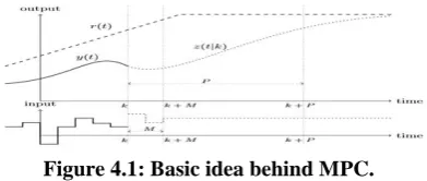
MPC is a process where an optimal output is obtained based on the predictions made by the results of input values using optimisation techniques with the help of minimised cost function. The optimisation techniques can be utilised in handling its problems through optimisation algorithms. The only disadvantage in implementing this predictive control strategy is that choosing the best optimal minimised cost function. Model-Based Prediction Control technique will be explained in this section [7]. First its essential standards will be presented. Next, output forecasting is done and the cost function is defined. Since those components of the MPC issue are treated in a somewhat different manner from the standard methodology they will be introduced in details [8]. There is much advancement in the MPC techniques that undergo the chain process of improvement in them. The basic principle which is involved in MPC is explained in the figure 4.1.

Figure 4.1: Basic idea behind MPC.

Having defined a reference direction for the plant’s output r(t) we need to follow it in optimal manner. To be specific, we need to adjust between the error occurred due to parameter identifying the traced error and the remaining parameters. In the present testing moment the direction of estimated output z(t|k) is being determined. It speaks to the style where the reference direction r(t) ought to be come to by the output signal y(t). It is defined over a specific number of future samples named the expectation horizon P. The plant data input, which are necessary for driving the system along with forecast direction z(t|k), are thought to change over a specified number of samples, called the control

horizon M, and remain steady a while later. With the awareness of the plant dynamics, representing a model for describing output evolution formulation over a specified predictive horizon P is derived. Following is, a cost function, depicting the optimal, from the originators perspective, balance between particular characteristics of the plant's behaviour, is defined. It is usually not a simple task since the individual control goals which are reflected there are opposite in nature. The estimation of the choice vector that limits the cost function is, in principle, the one that will enable the system to follow the trajectory of the predicted vector z(t|k) in the manner in which that is almost satisfied. It commonly comprises of the estimations of the present and future values of inputs to the system ∆U(k) however can also involve remaining variables.When a lot of future contributions to the system have been registered just the first one is given to the plant. In the following iterations of the calculation (at time k + 1) the cycle will iterate again. Both expectation P and control M horizon will be moved forward in time (yet will protect their length) by one example, new arrangement of future inputs will be acquired and again just the first one will be utilized. This methodology is known as the receding horizon strategy. The estimation of the systems output formulae and the entire clear description of how to minimise the cost function, as in case of MPC which is called quadratic programming problem are discussed in [9].

V. QUANTITATIVE FEEDBACK THEORY

Quantitative Feedback Theory which is a technique of frequency domain is introduced by Isaac Horowitz, which is widely utilized to attain a required robust design of a plant uncertainty within a specified region. QFT methodology of design was first developed for SISIO and LTI systems. Now a day, it is widely extended to many non linear systems, MIMO systems, time varying systems, discrete and non minimum phase systems also. QFT is a control engineering method of design that utilizes the feedback to minimize the effects of uncertainty of any plant and to have performance control specifications to be satisfied. Thus, QFT is being applied to large variety of real control problems successfully.

We consider a plant to perform this QFT analysis. Here we describe the plant with the transfer function as below: (2.25𝑠+18

𝑠 )(

16.4𝑠+1

0.25𝑠+1). ……….14

Fig.5.1.Summary of QFT design methodology. VI. SIMULATION RESULTS

Simulation process is carried out with two different input wind speeds like 12m/s and 16m/s. The various parameter variations are carried out and compared them in the simulation for three different controllers like MPC, QFT and PID. At both speeds mentioned above the parameters variations are shown below graphs as follows:

Fig 6.1 Input wind speed of 12m/s given to the system with respect to time variation.

Fig 6. 2 Torque versus time variation w.r.t different controllers.

We can observe more oscillatory behaviour with MPC and that is reduced in the case of QFT and PID.

Fig 6.3 Generator speed variation w.r.t time. The oscillatory nature of MPC is minimized using better

controllers like QFT and PID.

Fig 6.4 output power variation with time for all controllers is analysed.

Fig 6.5 pitch angle deviation in comparison to all controllers is performed.

Fig 6.6 wind speed variation of 16m/s with respect to time as an input to the system.

Fig 6.7 a time domain analysis of torque deviation is carried out in simulation.

Fig 6.8 generator speed characteristics in variation with time. As almost all controllers shows the similar behaviour but the MPC attains high peek overshoot.

Fig 6.9 output power versus time is simulated and observed that unity power is obtained at the same time

with more overshoot in MPC compared to other.

Fig 6.10 pitch angle variation is the major constraint which is improved in a better manner with QFT than

MPC. Comparison of parameters with 12m/s: Table 6.1 variation of parameters with torque.

Torque MPC QFT PID

tr(sec) 3.5 3.5 5

ts(sec) 45 35 40

Peak

overshoot(%)

50 25 12.5

International Journal of Innovative Technology and Exploring Engineering (IJITEE) ISSN: 2278-3075, Volume-8 Issue-12, October 2019

Generated speed

MPC QFT PID

tr(sec) 5 5 5

ts(sce) 42 33 28

Peak

overshoot(%)

16.67 6.67 8.33

Table 6.3 variation of parameters with output power. Output

power

MPC QFT PID

tr(sec) 5 5 5

ts(sce) 40 33 27

Peak

overshoot(%)

20 10 20

Table 6.4 variation of parameters with pitch angle Pitch

angle

MPC QFT PID

tr(sec) 9 7 6

ts(sce) 48 42 45

Peak overshoot (%)

50 10 20

Comparison of parameters with 16m/s:

Table 6.5 variation of parameters with torque.

Torque MPC QFT PID

tr(sec) 6 4 3.8

ts(sce) 40 40 40

Peak

overshoot(%)

35 25 20

Table 6.6 parameters with generated speed

Generated speed MPC QFT PID

tr(sec) 6 4.5 4.5

ts(sce) 40 40 40

Peak

overshoot(%)

16.67 6.67 3.33

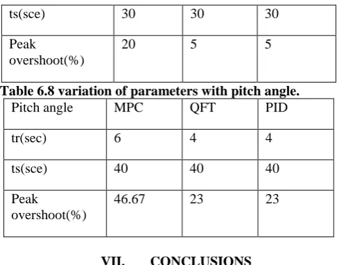
Table 6.7 Variation of parameters with output power.

Output power MPC QFT PID

tr(sec) 4 4 4

ts(sce) 30 30 30

Peak

overshoot(%)

20 5 5

Table 6.8 variation of parameters with pitch angle.

Pitch angle MPC QFT PID

tr(sec) 6 4 4

ts(sce) 40 40 40

Peak

overshoot(%)

46.67 23 23

VII. CONCLUSIONS

From overall comparison of various parameters like rise time(tr), settling time(ts) and peak overshoot(%) for the three different controllers like MPC, QFT, PID, we observe that MPC have more oscillatory nature of behaviour when compared with both QFT and PID. We can say that even the settling time taken by the system is more for MPC. Thus we can conclude that QFT with PID have more dynamic behaviour with respect to MPC.

REFERENCES

1. F.D. Bianchi, Hern´an De Battista, and R.J. Mantz. Wind Turbine Control Systems. Principles, Modelling and Gain Scheduling Design. SpringerVerlag, 2007.

2. Jogendra Singh Thongam and Mohand Ouhrouche. MPPT Control Methods in Wind Energy Conversion Systems.

3. L.C. Henriksen. Model predictive control of a wind turbine. Master’s thesis, Technical University of Denmark, 2007.

4. Bououden, S., Chadli, M., Filali, S., & El Hajjaji, A. (2012). Fuzzy model based multi variable predictive control of a variable speed wind turbine: LMI approach. Renewable Energy, 37,434–439. 5. Soliman, M., Malik, O. P., & Westwick, D. T. (2011). Multiple model

predictive control for wind turbines with doubly fed induction generators. IEEE Transactions on Sustainable Energy,2(3),215–225. 6. Gosk, A. (2011). Model predictive control of a wind turbine (Master’s

thesis).Technical University of Denmark

7. Mayne, D. Q. (2014). Model predictive control: Recent developments and future promise. Automatica, 50, 2967– 29

8. M.A. Henson, “Non linear model predictive control: Current status and future directions,” Comput. Chem. Eng., vol.23, pp.187– 202,1998.

9. J.M. Maciejowski. Predictive Control with Constraints. Prentice Hall, 2002

10.Garcia-Sanz and Houpis (2012), Houpis et al. (2006), Sidi (2002), Yaniv (1999), and Horowitz (1993)

AUTHORS PROFILE:

Y. Bharathi Devi born in Kadapa city, Andhra Pradesh, India in 1996. Received Graduation degree in Electrical and Electronics Engineering from JNTU PULIVENDULA, Andhra Pradesh in 2017. Currently doing Post Graduation in Electrical Power systems from JNTU, Anantapur.