City, University of London Institutional Repository
Citation
:
Mamouei, M. H., Kaparias, I. and Halikias, G. ORCID: 0000-0003-1260-1383 (2018). A framework for user- and system-oriented optimisation of fuel efficiency and traffic flow in Adaptive Cruise Control. Transportation Research Part C: Emerging Technologies, 92, pp. 27-41. doi: 10.1016/j.trc.2018.02.002This is the accepted version of the paper.
This version of the publication may differ from the final published
version.
Permanent repository link:
http://openaccess.city.ac.uk/id/eprint/19839/Link to published version
:
http://dx.doi.org/10.1016/j.trc.2018.02.002Copyright and reuse:
City Research Online aims to make research
outputs of City, University of London available to a wider audience.
Copyright and Moral Rights remain with the author(s) and/or copyright
holders. URLs from City Research Online may be freely distributed and
linked to.
A framework for user- and system-oriented optimisation of fuel
efficiency and traffic flow in Adaptive Cruise Control
Mohammad Mamouei ([email protected])
Ioannis Kaparias
George Halikias
Abstract
Fully automated vehicles are expected to have a significant share of the road network traffic in the
near future. Several commercial vehicles with full-range Adaptive Cruise Control (ACC) systems or
semi-autonomous functionalities are already available on the market. Many research studies aim at
leveraging the potential of automated driving in order to improve the fuel efficiency of vehicles.
However, in the vast majority of those, fuel efficiency is isolated to the driving dynamics between a
single follower-leader pair, hence overlooking the complex nature of traffic. Consequently fuel
efficiency and the efficient use of the roadway capacity are framed as conflicting objectives, leading
to fuel-economy control models that adopt highly conservative driving styles.
This formulation of the problem could be seen as a user-optimal approach, where in spite of
delivering savings for individual vehicles, there is the side-effect of the deterioration of traffic flow.
An important point that is overlooked is that the inefficient use of roadway capacity gives rise to
congested traffic and traffic breakdowns, which in return increases energy costs within the system.
The optimisation methods used in these studies entail high computational costs and, therefore,
impose a strict constraint on the scope of problem.
In this study, the use of car-following models and the limitation of the search space of optimal
strategies to the parameter space of these is proposed. The proposed framework enables
performing much more comprehensive optimisations and conducting more extensive tests on the
collective impacts of fuel-economy driving strategies. The results show that, as conjectured, a
“short-sighted” user-optimal approach is unable to deliver overall fuel efficiency. Conversely, a
system-optimal formulation for fuel efficient driving is presented, and it is shown that the objectives
of fuel efficiency and traffic flow are in fact not only non-conflicting, but also that they could be
1.
Introduction
During the past decade, environmental concerns have placed the energy efficiency of
vehicles at the centre of researchers’ efforts. Great leaps have been made in this area by
employing a wide range of technologies that improve fuel efficiency, such as the use of
lighter materials in car manufacturing, the adoption of more aerodynamic designs, and the
introduction of techniques such as pulse and gliding. However, an important factor that is
somewhat overlooked is the impact of the behaviour of drivers and of driving strategies on
fuel consumption. A search of the relevant literature reveals that this could be due to the
difficulties associated with the formulation of energy efficiency in the car following regime.
The algorithms proposed in this area are sometimes based on simplistic assumptions and
usually lack comprehensive investigations on their collective impacts and stability features.
This is due to the fact that the proposed models often rely on complex and computationally
demanding machine learning and optimal control theory-based methods, which make their
use in large-scale simulations impractical.
In this study, a new approach is proposed which makes use of car-following models in
optimisation. The use of car-following models as the basis of control has already been
addressed in the literature (Kesting, et al., 2010). The incorporation of car-following models
in simulation-based optimisation significantly reduces the complexity of the latter, which
then allows its application to much more comprehensive scenarios. Additionally, the
provision of control on the basis of car-following models benefits from the remarkable
advantage of the extensive knowledge that exists on the collective properties of these
models through the numerous studies that are available in the literature on aspects such as
stability features and traffic flow characteristics.
Two distinct approaches to the question of fuel efficiency are investigated in the present
study; 1. individual vehicles are considered and their fuel consumptions are minimised, and
2. fuel efficiency is considered from a broader, network-level perspective. While much of
the studies in the literature revolve around the former, the latter is somewhat overlooked.
A comprehensive analysis of the results sheds light on the important and fundamental
In section 2 a literature review is presented and subsequently the gap in the literature is
identified. In section 3 two new approaches for optimisation of fuel consumption are
formulated to cope with the shortcomings of the existing approaches. In section 4 the
results are presented. Finally, conclusions and future work are presented in section 5.
2.
Literature review
Wu et al. (2011) developed an advisory system that minimised fuel consumption in the
acceleration phase before reaching desired velocities and the deceleration phase before
coming to a standstill. The system was shown to deliver reductions of 12% to 31% in fuel
consumption and the objective was defined as the minimisation of the cumulative fuel
consumption, given by the VT-micro instantaneous fuel consumption model (Ahn, 1998),
within the time interval of interest (deceleration/acceleration period). For this purpose the
objective function was discretised and the resulting optimisation problem was then solved
using the Lagrange Multiplier Method (LMM).
Themann et al. (2015) proposed a control model for Adaptive Cruise Control systems (ACC)
that relied on the optimisation of the velocity profile with respect to fuel consumption. This
study used Dijkstra’s algorithm to find the optimal velocity profile for known road
topography. Porsche’s Innodrive ACC has also adopted a similar approach, resulting in about
10% reduction in fuel consumption (Markschläger, et al., 2012). Hellström et al. (2010)
developed a fuel-optimal control model for trucks. In this study, prior knowledge of road
topography was used in order to optimise fuel consumption and gear-shifting, and the
problem was formulated as a dynamic programming optimisation. In all these studies, fuel
economy is obtained by producing a smooth velocity performance and avoiding
unnecessary accelerations. Kohut et al. (2009) achieve the same objective by adopting a
Model Predictive Control (MPC) framework. This study highlights the trade-off between fuel
savings and trip time.
The development of optimal fuel economy control models in the car-following regime of
driving is a more challenging task due to the highly unpredictable nature of drivers’
behaviours. In the study by Li et al. (2008), cars’ tracking capabilities and fuel efficiency were
considered in the development of ACC, and in order to ensure fuel efficiency, accelerations
optimisation, and the testing of the control model was carried out by considering its
performance in an urban driving scenario and a highway driving scenario; fuel savings of
8.8% and 2% were obtained in each scenario respectively. Kamal et al. (2013) developed an
MPC-based controller for the car-following regime that saved an average of 13% in fuel
consumption in urban driving scenarios. Similar approaches can be found in other studies
(Luo, et al., 2015; Zhao, et al., 2017).
Zhang & Ioannou (2006) designed a Proportional-Integral-Derivative (PID) controller for the
car-following regime for trucks. The proposed method reduced fuel consumption by
avoiding unnecessary accelerations and braking, and the objective of the controller was set
to track the velocity of the preceding vehicle while maintaining a specified range of spacing.
A different approach in tackling the problem of fuel efficiency is based on the use of new
technologies. The potential of technologies such as hybrid electric powertrains and
telematics, providing traffic-related information (Manzie, et al., 2007) and techniques such
as pulse and gliding (Li, et al., 2012) in the reduction of fuel consumption has been
investigated in the literature.
Considering studies seeking more fuel-efficient driving behaviour, two categories can be
defined. The first category includes studies seeking to optimise fuel consumption for simple
scenarios, where there are no additional complexities caused by interactions between
vehicles. In this case information about roadway topography or the position of traffic signals
is used in order to formulate an optimisation problem and obtain the optimal velocity
profile (Wu, et al., 2011; Themann, et al., 2015; Markschläger, et al., 2012; Hellström, et al.,
2010; Kohut, et al., 2009). The second category, on the other hand, consists of studies
targeting driving conditions, where interaction between vehicles is the defining factor in
driving behaviour. In these studies often simplistic assumptions are made about the
relationship between fuel consumption and acceleration or driving dynamics in order to
reduce the complexity of problem. More importantly, due to the computational cost of the
methods used and the natural complexity of the car-following regime of driving, these
studies often narrow down the scope of the problem to a single pair of follower-leader and,
therefore, overlook the potentially negative impacts of their proposed control strategies on
traffic flow and fuel consumption within the network (Li, et al., 2008; Kamal, et al., 2013;
3.
Methodology
The modelling of car-following behaviour has been an active area of research for more than
six decades. Simple models that effectively describe the microscopic and macroscopic
features of traffic have been developed and have been widely studied. As a result, a good
understanding of different aspects of these models, namely their collective features and
stability characteristics, has been established over the years. Some of these models are also
integrated in the control of partially automated vehicles. In the present study the potential
of these models is leveraged in order to develop a control model that is not only efficient
with respect to fuel consumption but also takes into account the collective impacts of the
control model on traffic flow.
3.1 The IDM Car-following model
The Intelligent Driving Model (IDM) car-following approach has been selected for the
present study on the basis of its merits. Specifically, the studies available on the
macroscopic and microscopic calibration of the IDM point to the good performance of this
model on both aspects (Treiber , et al., 2000; Treiber & Kesting, 2013; Punzo & Simonelli,
2007). Moreover, the IDM has a simple mathematical form with a small number of
parameters, each corresponding to a driving attribute. Finally, numerous studies are
available on different aspects of this model, such as calibration, stability and other
microscopic and macroscopic properties (Wilson & Ward, 2011; Kesting & Treiber, 2009).
The IDM model is given by the following general equation;
̇ [ ( ) ( ( )) ]
( ) √ √
( )
where, is the maximum acceleration, is the desired speed, is the acceleration
exponent, and determine the jam distances in fully stopped traffic and in high
densities respectively, is the safe time headway, and is the comfortable deceleration.
vehicle, , and the distance headway, . Finally, the output variable, ̇, determines the
acceleration of the subject vehicle.
3.2 Optimisation framework
The coefficients of car-following models can vary according to driving strategies. Given a
sufficient number of model parameters, one can reproduce a variety of driving strategies
simply by changing the value of model parameters. For example, one set of parameters can
represent a sporty driving style with intense accelerations and braking, while another set of
model parameters can deliver a more conservative driving style that is less sensitive to the
lead vehicle’s braking by maintaining sufficient spacing. In other words, a car-following
model with model parameters provides a space, where each point in this space may
be regarded as a distinctive driving style. Therefore, one can seek to find the set of model
parameters within this space that minimises an objective function of choice. In this light,
calibration studies may be regarded as attempts to find the representations of particular
driving behaviour, given by particular trajectories, within the space of model parameters of
car-following models.
It is important to note that the space of strategies that is represented by the space of model
parameters of a given car-following model is only a subspace of all possible driving
strategies. Constraining the search space to the space of model parameters of a
car-following model has two direct consequences, an advantage and a disadvantage. On the one
hand this approach limits the search space to a space where important criteria such as
safety, stability, and producing acceptable driving behaviour could be satisfied. This
significantly reduces the complexity of the optimisation and mitigates the so-called “curse of
dimensionality” that is often encountered in dynamic programming-based approaches. On
the other hand, car-following models have shortcomings. A single set of model parameters
cannot always produce a realistic driving behaviour. Similarly, one cannot expect a single set
of model parameters to always provide a fuel-efficient driving strategy in all driving
conditions. Nevertheless, similar to calibration studies, one can obtain model parameters
that can deliver fuel efficiency in particular driving conditions.
In this study, two new and distinctive approaches in achieving fuel efficiency relying on the
consumption for a pair of vehicles, or a platoon of vehicles, subject to microscopic
constraints on the vehicle headways so as to ensure an efficient traffic flow and adequate
tracking capabilities; and b) an optimisation approach of the total fuel consumption within a
link, subject to a direct constraint on the traffic throughput. Due to the highly nonlinear
formulation of the problem, simulation-based optimisation is carried out to investigate the
two approaches.
3.2.1 Microscopically formulated optimisation
First the problem of a single pair of follower-leader is considered. The objective is to find the
optimal model parameters of the IDM that minimise fuel consumption. For this purpose the
problem is formulated as follows. Given a particular trajectory of the leader, , the
objective is to find the model parameters, , for the IDM car-following model that result in
the minimum fuel consumption for the follower.
( )
( ) ( )
where, is the fuel consumption of the follower, calculated by a modified version of the
VT-micro model (Ahn, 1998). This model is discussed in section 3.3.
In order to ensure that the results have an acceptable tracking capability and meet
flow-related requirements, a wide range of constraints have been considered based on different
criteria suggested in the literature (Zwaneveld & van Arem, 1997; Bierstedt & et al., 2014;
Marsden, et al., 2001). The following constraints have produced good results and are,
therefore, selected in this study.
̅̅̅
( ) ( )
where is the time series of headways of the follower, ̅̅̅ is the mean value of this time
series, and and are constants. Since the definition of headway becomes problematic
in low velocities, a threshold of 18 is considered in the calculation of headways and the
The results obtained using Equation (2) have been observed to be highly sensitive to the
initial conditions and the trajectory of the leader. Therefore, the optimisation framework
has been modified to include a platoon of vehicles that follow the trajectory of the lead
vehicle. By doing so, string stability features are also implicitly incorporated within the
framework.
( )
∑ ( )
( )
subject to,
̅̅̅ ̅̅̅̅ ̅̅̅̅
( ) ( ) ( ) ( )
where is the number of vehicles in the platoon. Additionally, in order to further improve
the robustness of optimisation results, the optimisation framework has been further
modified to consider more than one trajectory for the leader.
( )
∑ ( )
( )
This optimisation formulation is depicted in Figure 1.
Figure 1 Schematic representation of the microscopic optimisation scenario
The problem formulation presented in this section is similar to studies related to the
car-following regime of driving that were addressed in the literature review section. This
approach is, in essence, a user-optimal approach in which individual vehicles seek to
minimise their individual fuel consumption while respecting certain constraints that ensure
The approach presented in this section does not address a key aspect of the road network,
that is the role of individual entities in forming the collective features of the traffic flow and
the mutual impacts that individual agents and their collective behaviour have on one
another. The system-optimal optimisation approach presented next captures such
user-system dynamics and mutual impacts.
3.2.2 Macroscopically formulated optimisation
For this purpose the horizon of the optimisation problem is broadened in order to,
1. impose macroscopic constraints on the traffic flow, as opposed to the microscopic,
headway-based constrains that were previously used, and
2. capture the fuel efficiency properties of the traffic flow in a broader sense than just a
platoon of vehicles.
The optimisation problem is modified to the following. Given a particular trajectory, , for
a stretch of a roadway of particular length, , for the simulation time of seconds, and given
the inflow rate of , the objective is to find the model parameters, , of the IDM
car-following model that result in the minimum fuel consumption within the link. This is shown
in Equation (6).
( )
∑ ( )
( )
subject to,
where the operator denotes expected value, ( ) is the fuel consumption of the
vehicle following the lead trajectory calculated by the fuel consumption model, is the
number of vehicles in the scenario, and is a coefficient that sets a minimum threshold for
the acceptable throughput as a percentage of the expected number of vehicles that enter
the scenario, which is equal to . The intervals at which vehicles enter the simulation
scenario are modelled with the exponential distribution with the average of This
Figure 2 Schematic representation of the macroscopic optimisation scenario
3.3 Modified fuel consumption model
The VT-micro fuel consumption model is specifically developed for investigations related to
the operational level of driving, since the only input variables of the model are
instantaneous velocity and acceleration (Ahn, 1998). Although the model has a relatively
simple structure compared to some other fuel consumption models reviewed in Faris et al.
(2011) and Zhou et al. (2016), its dual regime, exponential structure, and large number of
terms (16 for each regime), impose a significant computational cost on the optimisation. In
order to address this issue a simplified version of the model is developed. The original
model and the new simplified model are given by equations (7) and (8), respectively.
( ( ))
{
∑ ∑
∑ ∑
( )
( ) ( )
where is acceleration, is speed, and are model coefficients.
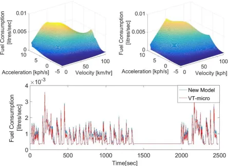
The new model is validated by comparing its estimates with the original model for the
Federal Test Procedure (FTP) drive cycle, which is representative of urban driving. The
results are demonstrated in Figure 3.
Figure 3 The comparison of fuel consumption prediction between VT-micro and the new model. a, b) Fuel consumption for the whole envelope of velocities and accelerations using VT-micro and the new model respectively. c) Instantaneous
fuel consumptions for the FTP drive cycle.
In spite of the much simpler equation of the new model, estimates that are sufficiently close
to the original VT-micro model are produced. In particular, the percentage error in total fuel
consumption for the FTP drive cycle using the new model is 10.4%, which, for the purposes
of fuel-consumption-based optimisation, can be deemed acceptable.
3.4 Datasets
Two datasets are used in this study: the reconstructed NGSIM-I80 (Montanino & Punzo,
2015) and the Naples (Punzo, et al., 2005) datasets. The NGSIM-I80 dataset provides
trajectory data extracted from a stationary camera that covers a 500-meter long stretch of a
six-lane highway, which allows the derivation of information about the traffic flow and the
overall fuel consumption. Because the original NGSIM-I80 dataset contains unrealistically
high accelerations which would bias the estimates of fuel consumption, a reconstructed
dataset is used in the present study. The Naples dataset, on the other hand, has been
obtained by instrumenting four vehicles and measuring their velocities and gaps while they
different sets of data, three of which report spacing and velocity values of the platoon of
vehicles while they drive through the three different routes, and the remaining two of which
obtained from two previously examined routes on different dates.
Unlike the NGSIM-I80 dataset, the Naples dataset does not provide any information about
the surrounding traffic conditions for the subject platoon; however due to the longer period
of trajectories for individual vehicles, the absence of lane changes, and the existence of
diverse driving conditions , the Naples dataset provides a better insight into car-following
behaviour compared to the NGSIM-I80 set. Therefore, in order to make the results of the
optimisations relevant to a broader spectrum of car-following conditions, the Naples
dataset is used here. The NGSIM-I80 dataset, on the other hand, is used as a reference case
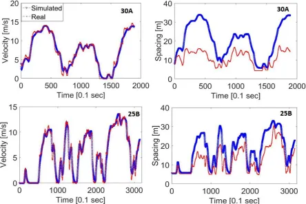
for validation purposes. Figure 4 depicts the velocity profiles of the platoon of vehicles in
[image:13.595.79.501.357.532.2]the Naples dataset for trajectories 25B and 30B.
Figure 4 Velocity measurements of the platoon of vehicles in the Naples datasets 25B and 30B.
In order to examine the impacts of the optimal driving strategies in different driving
conditions in the validation stage, two trajectories are extracted from lanes 1 and 2 of the
NGSIM-I80 dataset. Lane 1 is a High Occupancy Vehicle (HOV) lane and is not disturbed by
shockwaves. On the contrary, traffic in lane 2 is congested and numerous shockwaves
travelling upstream at a speed of 14 can be identified.
The first trajectory used in validation is drawn from lane 1 and relates to the vehicle with ID
441. This vehicle drives with the speed of about 90 . The second trajectory is extracted
of 18 and is subject to the main shockwave within the observation period. In the
simulations that are presented in section 4, these trajectories are used as the trajectory of
the first vehicle that enters the simulated roadway and the vehicles that follow it drive
according to the fuel-consumption-optimised models. The two different trajectories clearly
lead to different conditions for the following vehicles; the way in which these conditions
[image:14.595.74.520.224.386.2]affect the flow of vehicles and fuel consumption is examined in section 4.
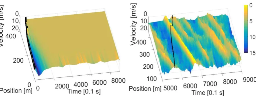
Figure 5 NGSIM-I80 dataset. Trajectories of a) the vehicle with ID 441 from lane 1 and b) the vehicle with ID 1845 from lane 2
The frequent occurrence of lane changes in the NGSIM-I80 dataset poses a challenge for the
evaluation of fuel consumption within a lane. Hence, fuel consumption results pertaining to
the real case are calculated from the vehicles that remain in the subject lane for the whole
period of observation. This is depicted in Figure 6.
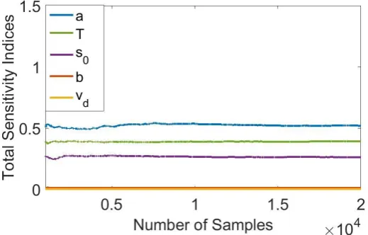
[image:14.595.161.421.567.736.2]3.5 Sensitivity Analysis
In order to further reduce the complexity of the optimisation a sensitivity analysis is
conducted to identify the parameters that have the highest impact on fuel consumption. In
this study, the global sensitivity framework is adopted, details of which and of its application
to the calibration of car-following models can be found in the litrature (Ciuffo, et al., 2014;
[image:15.595.159.419.263.429.2]Saltelli, et al., 2010; Jacques , et al., 2006; Punzo, et al., 2015). The result is illustrated in
Figure 7Error! Reference source not found..
Figure 7 Total sensitivity indices for the effects of the IDM model parameters on fuel consumption in a scenario where the trajectory of the leader is that of the leader in the Naples dataset 25B
It can be seen that parameter has the highest impact on fuel consumption, followed by
parameters and . Parameter has a negligible impact on fuel consumption and is
therefore set to its default value of throughout this study. Parameter has a
higher impact on fuel consumption compared to parameter . However, along with
define the spacing between vehicles. Since the two parameters are correlated (Jiwon &
Mahmassani, 2011) and the impact of on spacing is also captured by , parameter is
also set to its default value of 2 m. Although this sensitivity analysis suggests that parameter
has a marginal impact on fuel consumption, this parameter together with have a strong
impact on the stability features of the IDM. Therefore is also included in the optimisation.
Table 1 demonstrates the lower and upper bound values used in the sensitivity analysis. The
same bounds are used for parameters and in the optimisations. The results of the
Table 1 Lower and upper boundaries used and total sensitivity indices
Total sensitivity indices for datasets:
Parameters LB UB 25B 25C 30A 30B 30C
0.5 5 52% 37% 85% 82% 77%
0.5 5 1% 1% 2% 4% 2%
20 33 0% 2% 1% 0% 0%
2 5 26% 2% 7% 17% 18%
0.5 2 39% 60% 21% 14% 30%
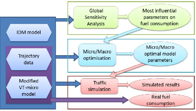
3.6 Overview of the methodology
The present study includes a number of components that were separately described in
section 3. Figure 8 provides a schematic representation of how these components are used
within different stages of this study.
Figure 8 Schematic representation of the present study
The VT-micro-based fuel consumption model provides estimates of fuel consumption
throughout this study, i.e. in the simulated scenarios for the NGSIM-I80 and the Naples
trajectories. The top rectangle on the right-hand-side in Figure 8 corresponds to the
sensitivity analysis that was carried out in section 3.5. Based on this analysis the three IDM
model parameters, namely , and , are selected as the set of minimisers in the
optimisations. The rectangle in the middle on the right-hand-side depicts the optimisation
stage where the optimal sets of parameters are determined. The microscopic and
[image:16.595.137.461.367.550.2]right-hand-side corresponds to the validation stage. In this stage a number of scenarios are
simulated where vehicles drive according to the optimal model and the fuel consumption
values in the simulated scenarios are compared with fuel consumption in its corresponding
reference case, given by the NGSIM trajectories.
4.
Results
4.1 Microscopically formulated optimisation
In this section the results relating to the microscopically formulated optimisation problem
denoted by Equation (5) are reported. In order to ensure that the results are as robust as
possible and deliver fuel efficiency in a wide range of driving conditions, all the trajectories
available within the five Naples datasets are used as the trajectory of the lead vehicle in the
optimisation. Also, the number of vehicles in the platoon is set to 4, and parameters and
are set to 3 and 0.5 seconds respectively.
The setting of the values of and is a result of a thorough investigation conducted in
order to examine the mean and standard deviation of the headways in different driving
conditions and for different drivers within the Naples dataset. The mean and standard
deviation of headways averaged over the five Naples datasets and all drivers are 1.1 and 0.4
s respectively. These values are highest for the third driver in all five datasets and reach the
values of 1.7 and 0.5 s respectively in dataset 25B. Additionally, numerous combinations of
and have been tested and it has been confirmed that and produce
realistic driving behaviour. The micro-optimal parameters obtained using these parameters
and in a scenario where a platoon of three vehicles follow the leader, are
, , and .
The optimal set of model parameters results in a 12% improvement in the fuel consumption
of the three following vehicles compared to the total fuel consumption in all five Naples
datasets (3.43 litres in the simulated scenario and 3.78 litres in the real case, as estimated
by the simplified VT-micro model). The saving is higher in driving conditions where
accelerations, stops, and speeding are more dominant. For instance, the reduction in fuel
Figure 9 demonstrates the driving behaviour reproduced by the optimal set of model
parameters when the trajectory of the lead vehicle is that of the leader in datasets 25B and
30A.
Figure 9 a) position, b) velocity, c) acceleration and d) spacing profiles produces using the optimal parameters compared to the real ones for the when the trajectory of the lead vehicle
It can be seen that the high value of parameter has resulted in a more conservative driving
style, which demonstrates itself through large spacing and a smoother velocity profile.
Although such a conservative driving style contributes to the reduction of fuel consumption,
it also leads to a reduction of traffic capacity. The deterioration of the traffic capacity means
that congested traffic states, intense shockwaves and traffic breakdowns could all occur in
lower traffic flows, leading to an increase in fuel consumption for the system. The impact of
traffic congestion on fuel consumption was investigated in Treiber et al. (2008) and it was
found that traffic congestion could lead to an increase of about 80% in fuel consumption.
In order to investigate the collective impacts of adopting such driving strategy, a simulation
is carried out where the trajectory of the leader is that of vehicle with ID 1845 and the
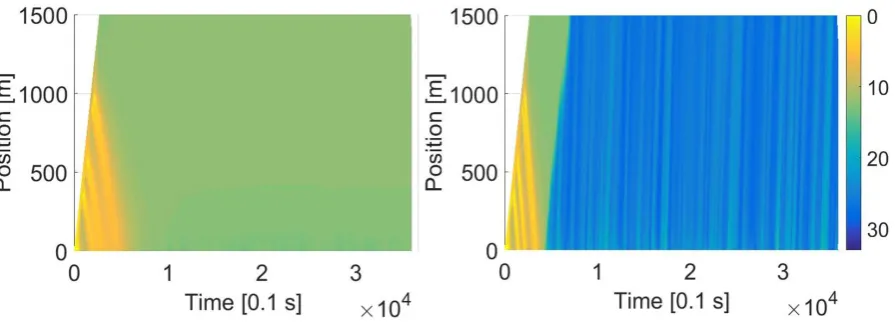
[image:18.595.76.521.153.449.2]1284 . Figure 10 compares the spatio-temporal velocity profile in the real scenario
[image:19.595.79.519.139.304.2]with the simulated one.
Figure 10 Comparison of the spatiotemporal velocity profile of the modelled scenario with the real data when the trajectory of the lead vehicle is =1845 (marked with the black solid line)
It can be seen that in the simulated scenario the shockwave triggers a homogenous
congested traffic state with an average speed of 14 . The analysis of the fuel consumption
in both scenarios shows that the user-optimal parameters, in spite of delivering fuel savings
for the immediate followers, lead to an increase in the average fuel consumption within the
link. In particular, the average fuel consumption for the 10 followers of the vehicle with ID
1845 in the real data is 10.5 . In the simulated dataset this value is reduced to 9.5
(average value in 100 simulations). However, the average fuel consumption for all
vehicles that follow the vehicle with ID 1845 is 10.3 in the real scenario, while for the
simulated dataset this is equal to 13.8 litres, i.e. a 34% increase in fuel consumption.
It is important to highlight the impact of the values of and on the optimal values. A
relaxation of these constraints leads to optimal parameters that have the following values:
the lower bound for parameter , the upper bound for parameter , and the upper bound
for parameter . While this combination of these values produces more savings for the
immediate followers, they result in a much more sluggish driving behaviour. Parameter
determines the headway and parameters and together define how agile the following
driver’s response is to changes in the velocity of the leader. High values of and low values
produce a driving behaviour that is much less sensitive to changes of the velocity of the
leader. A sluggish response to changes is beneficial for the fuel consumption of individual
vehicles.
The optimal parameters are also largely affected by the trajectory of the leader in the
optimisation. For instance, speeding and stops are much more present in dataset 25B
compared to dataset 30A, and the transition from stops to higher speeds occurs faster in
dataset 25B. The selection of trajectories from dataset 25B in the optimisation leads to the
optimal parameters , , and , while the selection of dataset 30A
leads to , , and .
As discussed, less sensitivity to changes of the velocity of leader generally contributes to
more fuel savings for individual vehicles. However, the optimal parameters for dataset 25B
( , ) produce more agile driving compared to the optimal parameters for
all five datasets ( , ). In order to address this contradiction, an analysis has
been conducted on the acceleration profiles produced by the two sets of parameters. This
analysis has revealed that in a driving condition in which changes in the velocity of the
leader occur frequently, such as dataset 25B, a less agile driving style produces accelerations
of smaller magnitudes. However, this also means that longer periods of
acceleration/deceleration must be performed to reach the desired speed, and this could
lead to an increase in the fuel consumption. Similar results, i.e. , and
, are found when the number of vehicles in the simulated platoon is increased to
Performing the optimisation using a number of trajectories from lane 1 of the NGSIM-I80
dataset, namely the trajectories belonging to vehicles with IDs 441, 452, 453, and 467,
confirms this finding. This set of trajectories belongs to a platoon of four vehicles that have a
steady speed during the observation period. The optimal parameters found in this case are:
, , and .
Microscopic simulation-based optimisation as described above, naturally, has its potential
1. The optimal values obtained, while producing savings for the immediate followers,
could be detrimental to traffic flow and thereby lead to an increase in fuel consumption
within the network. This is demonstrated in Figure 11, where a comparison is carried
out on the impacts of the model parameters on the flow. In one case the micro-optimal
parameters for the case of ( , , ) are used, and in the
second case the calibration results reported in Punzo & Simonelli (2007) are used. The
use of the calibrated model parameters from Punzo & Simonelli (2007) is particularly
interesting since in that study the same dataset (Naples dataset) was used for the
[image:21.595.76.524.300.462.2]calibration of the model parameters.
Figure 11 One-hour-long simulation with the inflow of 1800 . The trajectory of the leader is that of the leader in the Naples-25B dataset. a) The user-optimal parameters , the rest of the parameters are set to their default values, , , , b) The calibrated values from Punzo & Simonelli (2007), ,
, , ,
The results for the two scenarios are summarised in Table 2.
Table 2 The comparison of the micro optimal results with the calibrated set of model parameters from Punzo & Simonelli (2007)
Micro optimal
parameters when
Calibrated parameters (Punzo & Simonelli, 2007)
AFC within the scenario 8.12 7.18
AFC for 10 immediate followers 10.14 11.09
Traffic throughput 1298 1764
¹AFC=Average Fuel Consumption
2. Similarly to calibration studies, this type of optimisation is highly sensitive to the driving
[image:21.595.84.488.591.692.2]It worth mentioning that the evaluation of fuel consumption based on car-following models
that are purely calibrated with respect to individual trajectories or traffic may not produce
accurate results for individual vehicles. This subject is thoroughly discussed in Vieira da
Rocha et al. (2015). However, the same study concludes that fuel consumption estimates
are more reliable when the aggregate fuel consumption for platoons or the total traffic is
considered.
The results obtained in this section show that a user-optimal fuel economy driving strategy
can be characterised by high headway values. The relaxation of the headway requirements
yields the lower bound value for the acceleration parameter and the upper bound value for
the deceleration parameter. These parameters have the combined effect of maintaining
large spacing between the vehicles in order to afford less sensitivity to minor
brake/accelerations of the lead vehicle, hence producing smoother acceleration behaviour.
In terms of stability, low values of the parameter and high values of the parameter lead
to more instability, however, this is compensated by the increase in the value of the
parameter (Treiber & Kesting, 2011).
It is clear that increased values for parameter reduce the capacity of the roadway
however, this has a negligible impact on the traffic flow when the inflow of vehicles is low
and traffic is not in congested states. In other words, an increase in parameter does not
change the shape of the left branch of the fundamental diagram for the IDM car-following
model. However, as seen above, user-optimal optimisation remains oblivious to the broader
perspective of traffic flow and the strategies obtained using such narrowly-framed
optimisation formulations can lead to congested traffic states and traffic breakdowns, which
in return increase the cost of the trip in terms of fuel consumption within the network.
In what follows, a system-optimal formulation of the problem is presented, where a direct
constraint is placed on traffic throughput and the total fuel consumption within the system
is the subject of the minimisation.
4.2 Macroscopic optimisation
The objective of this section is to broaden the horizon of the optimisation scenario in order
1. impose macroscopic constraints on the traffic flow characteristics, as opposed to the
microscopic headway-based constraints that were previously used;
2. capture the fuel efficiency properties of the traffic flow in a broader sense than just a
platoon of vehicles; and
3. reduce the sensitivity of the optimal parameters to driving conditions.
For this purpose the optimisation framework described in sub-section 3.2.2 is applied here.
[image:23.595.127.507.272.451.2]The input values of the optimisation scenarios are given in Table 3.
Table 3 Features of the simulation scenarios used in the macroscopically formulated optimisations
1.2 – 2 according to the trip length in the Naples
datasets.
5 and 60 minutes.
[ ]
Different values within the range [1080 2664] and
with increments of 200.
trajectories from the datasets 25B, 25C, 30A, 30B,
and 30C, from the Naples dataset.
70%
Three simulation parameters are changed in the optimisation scenario in order to
investigate their impact on the optimal parameters: the inflow of vehicles, the trajectory of
the lead vehicle, and the simulation time. The variation of the inflow and the lead trajectory
allows investigating how robust the optimal parameters are to changes of traffic conditions.
The variation of the simulation time enables an assessment of how the consideration of fuel
efficiency as both a short-term and a long-term objective affects the optimal strategy.
The optimisation is carried out using a genetic algorithm. Running the optimisation takes
between one to three days on a High-Performance Computing (HPC) cluster. Each cluster
node consists of two 2.5Ghz Intel Xeon E5-2670v2 processors, with 40 processors dedicated
to the task.
For the short simulation time of the following optimal values are obtained:
these values are understandably similar to the user-optimal results with relaxed headway
requirements.
When the simulation time is extended to one hour the following parameters are obtained:
, , . Conversely to what was previously observed, the lower bound
value for headway is obtained, which ensures an increase in the capacity of traffic flow. The
upper bound value for the acceleration parameter and the lower bound value for the
deceleration parameter compensate the instability that arises from the low value of .
Interestingly the results are almost completely robust to changes of the leader’s trajectory,
variation of the inflow, and even further relaxation of the throughput requirement by
reducing to 50% (small variations in the value of parameter take place when the inflow
of vehicles goes above 2200 ). These results are somewhat counterintuitive, as the
driving behaviour produced using these parameters is highly agile, and this contradicts the
assumptions made in many studies.
Figure 12 demonstrates the comparison of the system-optimal parameters with the
user-optimal ones in a simulation where the trajectory of the first vehicle that enters the
scenarios is that of the leader in the Naples dataset 25B and the inflow of vehicles is 1800
. The flow-density diagrams are obtained by placing three virtual detectors at 500 m
intervals and using the equations below to calculate the average flow and density. The
derivation of the fundamental diagram for homogenous traffic is discussed in Treiber et al.
(2000).
̅ ∑
̅ ( )
where is the time interval equal to min, is the vehicle count at time interval , and
Figure 12 Spatio-temproal graph obtained when the macroscopically optimal parameters for the two-hour-long scenario are used, a) vehicle ID 441 b) = ID 362
The use of the system-optimal model parameters results in an average traffic throughput of
about 1800 and an average fuel consumption of about 6.68 , compared to the
traffic throughput of 1298 and the average fuel consumption of 8.12 for the
user-optimal parameters; this significant saving in the total fuel consumption comes at the
cost of a 12% increase in the fuel consumption of the 10 immediate followers of the first
vehicle entering the scenario. These values are obtained in a two-hour-long simulation and
are averaged over 100 independent simulations. This highlights the fundamental differences
between the two approaches to fuel efficiency.
Finally, Table 4 provides a comprehensive comparison of the results when the trajectories of
the vehicles with IDs 441 and 1845 (from the HOV lane and lane 2 respectively) are used in
the simulation. These values are obtained in one-hour-long simulations. The inflow of
vehicles is adjusted to the real scenario, that is 1284 for the scenario when
Table 4 Results obtained in different optimisations described previously for when the dataset Parameters’ values And results Micro, , , Micro , , Macro Macro Real
1.7 4.3 0.5 5 NA
1 3 5 0.5 NA
2 2 2 0.5 NA
Lead Vehicle ID 441 1845 441 1845 441 1845 441 1845 441 1845
AFC 7.1 13.8 7.3 14.2 8.5 11.3 6.4 6.9 6.9 10.3
AFC (10 followers) 6.7 9.5 6.3 9.4 6 11 7.6 10.1 6.3 10.5
TTh ¹ 1344 963 1344 937 1135 1075 1344 1284 1344 NA²
¹AFC=Average Fuel Consumption, TTH= Trafic Throughput
² Not possible to estimate due to the large number of lane-changes
5.
Conclusion and future work
In this study, a new framework for conducting user- and system-oriented optimisation
related to fuel efficiency in the car-following regime was presented. The framework builds
on the extensive literature available on car-following models and limits the search space of
optimisation to a sub-space of possible driving strategies that is modelled by a car-following
model. Depending on the car-following model, this sub-space could represent a search
space where important criteria of driving, such as stability, safety, comfort and driver
acceptability, are satisfied. Unlike the dynamic programming-based or
optimal-control-theory-based methods that can be seen in the literature, the proposed method allows
performing large-scale, scenario-based optimisation, and testing the impacts of optimal
strategies on the collective features of traffic flow. In this study the focus was on fuel
consumption, while other objectives can also be investigated within this framework.
Firstly, similarly to numerous studies in the literature, the question of fuel efficiency was
formulated as the minimisation of the fuel consumption of a vehicle (or a small number of
vehicles) while following the leader. The optimal parameters found using the proposed
approach produce a driving behaviour that is consistent with the control models proposed
in other studies. The optimal parameters yield a driving behaviour that ensures sufficiently
large gaps between the vehicles. Furthermore, this strategy is insensitive to minor
user-optimal driving strategy that, while delivering savings for the immediate followers,
leads to a drastic deterioration of traffic capacity. Consequently, the fuel costs of trips
significantly increase within the network.
The relationship between fuel consumption and traffic flow is a complex one. Adopting
narrowly framed optimisation frameworks based on a single pair of vehicles cannot
adequately capture the complex nature of traffic. In order to address this, a system-optimal
optimisation was formulated. The system-optimal driving strategy was shown to vary
significantly from the user-optimal one. In particular, the user-optimal driving strategy
encourages a sluggish driving style with large gaps between the vehicles, while the
system-optimal driving strategy encourages short headways and a highly agile driving behaviour,
leading to traffic flow efficiency, as well as network-wide reductions of fuel consumption.
The key finding of the present study is that the application of the user-optimal control
models that are widely seen in the literature may be suitable to free-flow conditions, but for
more congested states, as is commonly encountered in urban areas, a system-optimal
approach, like the one proposed, appears to be more appropriate. And while the study has
thrown some light into the topic of energy-efficient ACC, work in this direction continues.
Specifically, the next step of the research entails the consideration of the effects of lane
changing and of the heterogeneous nature of traffic, which were not addressed here. These
subjects and their impacts on the results will be thoroughly analysed in a future study,
where the model will be implemented in a realistic urban network consisting of mixed
traffic. Further future research will also investigate the use of other suitable car-following
models and the application of the framework to different objectives.
Acknowledgement
The paper highly benefited from the valuable comments of the anonymous reviewers. The
authors would also like to thank Dr. Vincenzo Punzo and Dr. Marcello Montanino for sharing
their remarkable work in the reconstruction of the NGSIM-I80 dataset and for providing the
Naples dataset.
The research reported has been supported by City University London’s Doctoral
Studentships scheme.
References
Ahn, K., 1998. Microscopic fuel consumption and emission modeling, Blacksburg: Civil and
Environmental Engineering. Virginia Polytechnic Institute and State.
Bierstedt , J. & et al., 2014. Effects of Next Generation Vehicles on Travel Demand and Highway
Capacity.[Online]
Available at: http://orfe.princeton.edu/~alaink/Papers/FP_NextGenVehicleWhitePaper012414.pdf
Ciuffo, B., Punzo, V. & Montanino, M., 2014. Global sensitivity analysis techniques to simplify the
calibration of traffic simulation models. Methodology and application to the IDM car-following
model. IET Intelligent Transport Systems, 8(5), p. 479 – 489.
Faris, W. et al., 2011. Vehicle fuel consumption and emission modelling: an in-depth literature
review. Intenational Journal of Vehicle Systems Modelling and Testing, Volume 6(3/4), pp. 318-395.
Hellström, E., Åslund, J. & Nielsen, L., 2010. Design of an efficient algorithm for fuel-optimal
look-ahead control. Control Engineering Practice, Special Issue on Automotive Control Applications, 2008
IFAC World Congress, 18(11), p. 1318–1327.
Jacques , J., Lavergne, C. & Devictor, N., 2006. Sensitivity analysis in presence of model uncertainty
and correlated inputs. Reliability Engineering & System Safety, 91(10-11), p. 1126–1134.
Jiwon, K. & Mahmassani, H. S., 2011. Correlated Parameters in Driving Behavior Models:
Car-Following Example and Implications for Traffic Microsimulation. Transportation Research Record:
Journal of the Transportation Research Board, Issue 2249, pp. 62-77.
Kamal, A. S., Mukai, M., Murata, J. & Kawabe, T., 2013. Model Predictive Control of Vehicles on
Urban Roads for Improved Fuel Economy. IEEE Transactions on Control Systems Technology, 21(3),
pp. 831-841.
Kesting, A., Treiber, M. & Helbing, D., 2010. Enhanced Intelligent Driver Model to Access the Impact
of Driving Strategies on Traffic Capacity. Philosophical Transactions of the Royal Society A 368, pp.
Kohut, N. J., Hedrick, J. K. & Borrelli, F., 2009. Integrating Traffic Data and Model Predictive Control
to Improve Fuel Economy. Redondo Beach, CA, USA, Proceedings of the 12th IFAC Symposium on
Transportation Systems.
Li, S. E., Peng , H., Li , K. & Wang, J., 2012. Minimum Fuel Control Strategy in Automated
Car-Following Scenarios. IEEE Transactions on Vehicular Technology, 61(3).
Li, S. et al., 2008. MPC based vehicular following control considering both fuel economy and tracking
capability. s.l., Vehicle Power and Propulsion Conference. VPPC '08. IEEE .
Luo, Y., Chen, T., Zhang, S. & Li, K., 2015. Intelligent Hybrid Electric Vehicle ACC With Coordinated
Control of Tracking Ability, Fuel Economy, and Ride Comfort. IEEE TRANSACTIONS ON INTELLIGENT
TRANSPORTATION SYSTEMS, 16(4), pp. 2303-2308.
Manzie, C., Watson, H. & Halgamuge, S., 2007. Fuel economy improvements for urban driving:
Hybrid vs. intelligent vehicles. Transportation Research Part C: Emerging Technologies February
2007, 15(1), pp. 1-16.
Markschläger, P., Wahl, H. G., Weberbauer, F. & Lederer, M., 2012. Assistance System for Higher
Fuel Efficiency. Auto Tech Review, 1(12), pp. 40-45.
Marsden, G., McDonald, . M. & Brackstone, M., 2001. Towards an understanding of adaptive cruise
control. Transportation Research Part C: Emerging Technologies, 9(1), p. 33–51.
Montanino, M. & Punzo, V., 2015. Trajectory data reconstruction and simulation-based validation
against macroscopic traffic patterns. Transportation Research Part B: Methodological 80, Volume 80,
pp. 82-106.
Punzo, V., Formisano , . D. J. & Torrieri, V., 2005. Nonstationary Kalman Filter for Estimation of
Accurate and Consistent Car-Following Data. Transportation Research Record: Journal of the
Transportation Research Board, Issue 1934, pp. 3-13.
Punzo, V., Montanino , M. & Ciuffo, B., 2015. Do We Really Need to Calibrate All the Parameters?
Variance-Based Sensitivity Analysis to Simplify Microscopic Traffic Flow Models. IEEE Transactions on
Intelligent Transportation Systems, 16(1), pp. 184 - 193.
Punzo, V. & Simonelli, F., 2007. Analysis and comparison of microscopic traffic flow models with real
traffic microscopic data. Transportation Research Record: Journal of the Transportation Research
Saltelli, A. et al., 2010. Variance based sensitivity analysis of model output. Design and estimator for
the total sensitivity index. Computer Physics Communications, 181(2), p. 259–270.
Themann, P., Bock, J. & Eckstein, L., 2015. Optimisation of energy efficiency based on average driving
behaviour and driver’s preferences for automated driving. IET Intelligent Transport Systems, 9(1), pp.
50-58.
Themann, P. & Eckstein, L., 2012. Modular Approach To Energy Efficient DriverAssistance
Incorporating Driver Acceptance. Alcalá de Henares, Spain, s.n.
Treiber , M., Hennecke , A. & Helbing, D., 2000. Congested traffic states in empirical observations
and microscopic simulations. Physical Review E, 62(2), p. 1805–1824.
Treiber , M. & Kesting, A., 2011. Evidence of convective instability in congested traffic flow:
Asystematic empirical and theoretical investigation. Transportation Research Part B: Methodological,
45(9), p. 1362–1377.
Treiber, M. & Kesting, A., 2013. Microscopic Calibration and Validation of Car-Following Models – A
Systematic Approach. Noordwijk, Netherlands, s.n., p. 922–939.
Treiber, M., Kesting, A. & Thiemann, C., 2008. How Much Does Traffic Congestion Increase Fuel
Consumption and Emissions? Applying Fuel Consumption Model to NGSIM Trajectory Data.
Washington DC, s.n.
Vieira da Rocha, T. et al., 2015. Does traffic-related calibration of car-following models provide
accurate estimations of vehicle emissions?. Transportation Research Part D: Transport and
Environment, Volume 34, pp. 267-280.
Wu, C., Zhao, G. & Ou, B., 2011. A fuel economy optimization system with applications in vehicles
with human drivers and autonomous vehicles. Transportation Research Part D: Transport and
Environment, 16(7), pp. 515-524.
Zhang, J. & Ioannou, P., 2006. Longitudinal control of heavy trucks in mixed traffic: environmental
and fuel economy considerations. IEEE Transactions on Intelligent Transportation Systems , 7(1), pp.
92-104.
Zhao, R. C., Wong, P. K., Xie, Z. C. & Zhao, J., 2017. Real-time weighted multi-objective model
predictive controller for adaptive cruise control systems. International Journal of Automotive
Zhou, M., Jin, H. & Wang, W., 2016. A review of vehicle fuel consumption models to evaluate
eco-driving and eco-routing. Transportation Research Part D: Transport and Environment, Volume 49, pp.
203-218.
Zwaneveld , P. & van Arem, B., 1997. Traffic effects of Automated Vehicle Guidance systems, Delft,