The offshore access problem and turbine availability : probabilistic modelling of expected delays to repairs

(1)

The offshore access problem and turbine availability -

probabilistic modelling of expected delays to repairs

Feuchtwang JBא & Infield DGא

mailto:[email protected]

'phone +44 (0) 141 548 4343

א

Institute for Energy and Environment

Dept. of Electronic and Electrical Engineering Royal College Building

University of Strathclyde 204 George Street Glasgow G1 1XW

1 Introduction

Operation and maintenance can strongly affect the cost of energy from offshore wind-farms through its effect on lost energy production. Difficulty of maintenance access, particularly due to adverse sea-state, has a major impact on turbine availability, and there is a need for improved understanding of this effect. A probabilistic event-tree model has been developed as an alternative to conventional Monte Carlo methods that require repeated extensive simulations. Expected values of delays due to sea-state can be expressed as closed form expressions depending on the probability distributions of sea-state ‘storm’ and ‘calm’ duration. Using records of significant wave height, sea-state duration distributions for a given threshold wave height can be computed directly from level-crossings and ‘storm’ and ‘calm’ durations. Weibull distributions are generally a good fit for these distributions and relevant parameters can be calculated using maximum likelihood methods. The contribution from each branch of the event-tree to the expected delay time is a function of a small set of parameters calculated from the duration probability distributions. If these distributions are used in Weibull form, they can be calculated directly from the calm and storm duration Weibull parameters for the particular wave-height.

Using subsystem reliability and repair time data, a simple spreadsheet can then be used to estimate annual expected delays due to each subsystem as well as the sensitivities of delays to site, turbine and access parameters. In this work, subsystem reliabilities and repair times are based on operational data from Danish and German turbines based on land.

Assumptions are also made about access methods for repairing different subsystems and consequently permissible sea conditions.

Calculations for wind turbines located at North Sea sites for which wave data are available indicate that annual down-times are dominated by repairs to the blades, generator and gearbox. These are not necessarily the subsystems with the highest failure rates but those requiring long repair windows and whose repairs currently require large crane vessels, the use of which is severely restricted by sea-state. The greatest influence on down-time and availability is found to come from changes in the access conditions for repairs, by reducing reliance on ‘sensitive’ vessels, by reducing repair time at the turbine and by reducing vessels’ sensitivity to sea-state.

The advantage of the approach developed is that it is possible to explore the impact of changing access thresholds, reliabilities or site parameters quickly and easily without having to run a long series of simulations for each new situation.

2 Methodology for estimating access delays

The aim of this study is to arrive at estimates of non-availability of wind turbines recently and/or currently being installed offshore in Europe, overall and broken down by sub-system. The approach used is that of a probability ‘event tree’ in order to be able to look quickly at a wide range of input data and scenarios. Simplifying assumptions are made to keep the event tree manageable.

(2)

wave height Hth. It has further been assumed that the repair takes a certain time, treq and (perhaps simplistically) that the wave height restriction applies throughout that time. There are clearly other possible sources of delay, particularly the availability of suitable vessels, spares and personnel but these are outside the scope of the study at present.

2.1 Requirements for model

There are several possible approaches to modelling offshore access and its effect on operation and maintenance and thereby on turbine availability. Any such approach will always require certain key elements:

– wind and wave data

– failure rate data for each relevant component or sub-system and each type of failure.

– actions required in response to each type of failure, particularly materials, personnel, tools and plant and time needed and by implication the vessels to be used.

– the limiting operational conditions, expressed as threshold wind speeds and wave heights for safe operation (characteristic of the vessel required and the transfer systems).

– travel and operating times required

– a statistical model

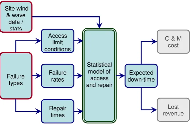
[image:2.595.143.451.335.538.2]

How these elements fit together in almost any model of offshore access is shown schematically in Figure 1.

Figure 1: Schematic diagram of offshore access delay calculation

The most widespread method of estimating offshore delays and system down-time is to employ Monte Carlo methods. The advantage of the Monte Carlo method is that quite complex strategies and scenarios can be modelled. The disadvantages are that many long runs are required to achieve any statistically significant results and that uncertainties are not very ‘transparent’.

A more direct approach to modelling delays is to construct an ‘event tree’. This describes every conceivable event and its alternatives, prerequisite conditions and consequences, with probabilities assigned to each ‘branch’. The advantage is transparency and speed and simplicity of computation and this makes it straightforward to explore trends by varying input parameters. However, the event tree can rapidly become hard to manage as complexity increases.

2.2 Probabilistic delay model

The probabilistic model of operational delay developed here is based on a number of simplifying assumptions that, for the sake of clarity, allow the presentation of a very simple event tree and the derivation of relatively simple expressions for expected delay. However,

Site wind & wave

data / stats

Failure types

Access limit conditions

Failure rates

Repair times

Statistical model of

access and repair

Expected down-time

O & M cost

(3)

this is by no means exhaustive and the same principles can be applied with care to more complex event trees.

For any given offshore operation, the starting point is to define the wave statistics of the given site, the operational limits, which may be expressed as a limiting or threshold wave height for the given vessel, as well as the operation time required (consisting of travel time plus repair time). The expected or mean delay time can then be calculated and thereby down-time. A number of assumptions have been made:

– Faults occur randomly and independently.

– Offshore, after a lead time for preparation, mustering etc., the aim is to travel to the turbine, transfer, carry out the repair in one go, transfer back and return to land, and to avoid multiple trips for any one repair.

– Only a single operational limit applies to each operation considered, in this case, significant wave height. Although a more comprehensive model would also consider wind speed as a limiting condition, this has been left out for simplicity. 1

– Short term forecasts of sea state are assumed to be available up to at least the period of time corresponding to the length of the required operation. An operation should only be initiated when the sea-state is forecast to be favourable for a sufficient time. It would be unsafe to leave a crew stranded on the turbine in a high sea-state. It would also be unacceptable to leave a repair incomplete unless unavoidable through mistaken forecasts of unexpected difficulties and delays with the repair. In reality this is possibly too restrictive, though probably more realistic and acceptable than repairs being left unfinished between periods of hostile seas. It may, however, be possible to plan the splitting of some of the longer repairs into multiple sessions.

Modelled outcomes:

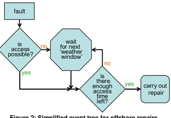
The event tree can be represented as in Figure 2 below. This accounts both for the threshold wave height and the required time window and is deceptively simple.

fault

is access possible?

is there enough access time left? wait

for next ‘weather window’

carry out repair

no

yes yes

[image:3.595.163.438.400.589.2]

no

Figure 2: Simplified event tree for offshore repairs

Even with this tree, it is possible to identify 4 distinct situations when a fault occurs (see Figure 3):

0: the sea state is low enough and there is sufficient time left to carry out the operation (no delay)

1: the sea state is too high to gain access. The next period of low sea must be waited for. (1st order delay)

1_{Wind speed and wave height are generally quite well correlated at any given site, albeit differently at each site, as}

(4)

2a: the sea state is low enough but is predicted to be too short to effect repair. This period and the subsequent period of high sea-state must be waited through. (2nd order delay, type a)

2b: the sea state is low enough and the predicted period is long enough but there is insufficient time left in the current period to complete the operation, ie the fault occurred too late in the weather window. As above, this period and the subsequent period of high sea-state must be waited through. (2nd order delay, type b)

In the event of high waves, eventually there will be a period of suitably low wave height but it too may or may not be long enough to effect the repair. If not, this would lead to a further cycle of delays. Similarly, after a 2nd order delay, there will be a period of high waves followed by a period of low waves and as above this may or may not be long enough.

Figure 3: Example wave-height time-series with illustration of types of delay

The probabilities of occurrence of periods of different duration as expressed in the probability distribution are based on numbers of occurrences expected in, say, a year. In contrast a fault is more likely to occur in a long period than a short one so whether an initial fault occurs in period of type 0, 1, 2a, or 2b, must be time biased. Thus, the expectation of delay resulting from the fault is determined by the ‘time-biased’ ‘storm’ (exceedence) and ‘calm’ (non-exceedence) duration probability distributions. On the other hand, the probability of a subsequent period being long or short is not biased in this way and, assuming independence2, follows the original unbiased occurrence probability distribution.

The derivation of the relevant expressions for the probabilities of each of the above and the respective expected values of delays is omitted here but will, it is hoped, be published at a later date. The resulting expression for expected delay is calculated directly from the probability distributions of the wave height itself, and of calm and storm durations for the threshold wave height being considered. It consists of probabilities, mean durations and 1st and 2nd moments of the distributions – all standard calculations from a probability distribution. The expected value of the delay, taking into account all contributions, and with arguments omitted for clarity, is given by

E

(

t_delay

(

H_th, t_req

)

P

⋅

(

t_req−τ_x

)

+

P M

⋅ _qqx⋅τ_x

(

1−

P

)

2

P

⋅

M

qqn⋅τx

+

P Q

⋅ _n treq

2

2⋅τ_x

⋅ +

(

1−

P

)

⋅

M

_qn⋅treq

P

+

(

1−

P

)

⋅

M

_qn





2

P Q

⋅ _n

τ_x ⋅ +

+

...

{1}

2

This assumption of statistical independence is essential for realisable calculation. 0.0

0.5 1.0 1.5 2.0 2.5 3.0 3.5 4.0

13/10 18/10 23/10 28/10 02/11 07/11

0.0 0.5 1.0 1.5 2.0 2.5 3.0 3.5 4.0

13/10 18/10 23/10 28/10 02/11 07/11

0.0 0.5 1.0 1.5 2.0 2.5 3.0 3.5 4.0

13/10 18/10 23/10 28/10 02/11 07/11

date

s

ig

n

if

ic

a

n

t

w

a

v

e

h

e

ig

h

t

H

s

(

m

)

After 1, 2a or 2b, low sea-state periods may again be too short leading to more delays

0: repair can go

ahead

2a: period too short 2b: fault

too late required

Hth , t

)

up to treq. The outcome of the probability tree calculation is a set of curves giving delay time as a function of limiting sea-state (threshold wave height) and operational time required. An example family of curves in Figure 4 is based on the same Dowsing site data used later in time series calculations. They show delay time against operation time for a range of

threshold wave heights. It can be seen that the delay time is very sensitive to both operation time and threshold. It should also be noted that they are highly sensitive to the specific site’s sea conditions.

0 2 4 6 8 10

0 10 20

0.6 m 0.8 m 1.0 m 1.2 m 1.5 m 1.8 m 2.0 m 2.5 m 3.0 m

repair time (days)

ex

p

ec

te

d

el

a

y

t

im

e (

d

a

y

s)

Figure 4: Expected delay time vs repair time, for different wave height thesholds

2.3 Wave data and statistics

The expressions for probabilities and expected delays can be calculated in different ways depending on the type of wave data available.

2.3.1 Time series data

Records of measured wave time-series data are the ideal source. It might be argued that in that case, one should simply time-step through the data series and simulate fault occurrence using Monte-Carlo methods. However, as has been mentioned before, this requires multiple runs, each of which should use a different run of data, in order for results to be credible. It is rare for such long runs of data to be available. Obviously, using any method, the results can be expressed with a greater degree of confidence when based on a long data series. However, it is still possible to derive useful statistics using shorter runs as long as it is done with caution. It is even possible to derive statistics from an aggregation of several shorter data runs.

An alternative to measured data is to employ so-called hindcast data. The NESS, NEXT and NEXTRA studies ([1], [2]) used wave generation, propagation and attenuation models with Bathymetric data and forcing from recorded Meteorological data in order to hindcast a potentially complete ‘record’ of winds, waves, currents and water levels for the North

(6)

0 1 2 3 0

0.2 0.4 0.6 0.8

0 0.2 0.4 0.6 0.8

numerical prob dens Weibull fit pdf numerical exc prob Weibull fit xp

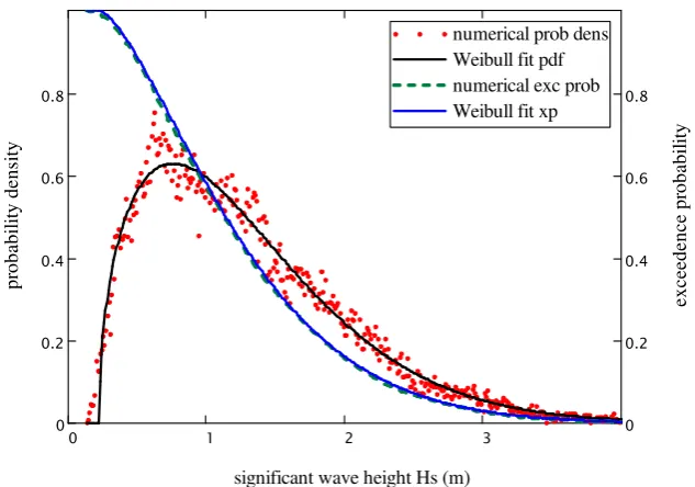
Wave height distribution from Dowsing - Weibull fit (ML)

significant wave height Hs (m)

p

ro

b

a

b

il

it

y

d

e

n

si

ty

e

x

c

e

d

e

n

c

e

p

ro

b

a

b

il

it

[image:6.595.140.457.79.301.2]

y

Figure 5: Numerical distribution of significant wave height and Weibull fit

Given time-series data, it is relatively straightforward to generate a numerical probability distribution of wave height directly, both in the form of probability density,

p(

Hth

)

,and cumulative/exceedence probability

P(

Hth

)

. The former tends to be somewhat noisy, as can be seen above in Figure 5 but this does not matter as it is never used in its ‘raw’ form; it is only ever used in integrations in order to calculate other statistics. Data used here is from the Dowsing site from Nov 2005 to Jan 2008, and was downloaded from CEFAS’s Wavenet web-page [3].

0.1 1 10 100 1 10× 3

0 0.2 0.4 0.6 0.8 1

calm numerical exc prob calm Weibull exc prob calm K-H exc prob

Wave height calm duration from Dowsing, Hth = 2m calm duration (hr)

e

x

c

e

d

e

n

c

e

p

ro

b

a

b

il

it

y

Figure 6: Numerical calm duration distribution with Weibull fit and K&H estimate

The remaining statistics require the use of a level-crossing detection algorithm. For any given threshold wave height, the time series is divided up into periods above and below the

threshold, or storms and calms, as shown in the pink line in Figure 3. The durations of the periods are calculated and assembled into 2 numerical distributions, for storms and for calms,

[image:6.595.147.447.435.613.2]

(7)

2.3.2 Fitting Weibull parameters to time series data

An alternative approach is to fit probability distribution functions to the numerical wave height distribution and to the calm and storm duration distributions for the relevant threshold wave height. There is no unique approach to this but it has generally been found that Weibull distributions are a reasonably good fit to (non-extreme) wave data [6,7,8,9 and others]. For the significant wave height distribution, it is generally best to employ a 3-parameter fit, having a location parameter, a scale parameter, and a shape parameter.

In general, the preferred method of fitting parameters is the maximum-likelihood method, though it is difficult to find a stable result when estimating all 3 parameters and at least one author describes it as mathematically impossible [4]. Least squares and least distance methods suffer from similar difficulties. According to Cran [5], it is possible to use moment methods, which yield a stable, though unfortunately inaccurate, result. Once a location parameter has been estimated, maximum likelihood estimation of the scale and shape parameters is straightforward.

The storm and calm duration distributions present less of a problem as only 2 parameter fits are necessary and the maximum-likelihood method is ideal.

Once these distributions have been fitted to the data, calculation of the 6 relevant quantities follows directly from standard probabilities and moments of the Weibull distribution, involving the exponential and gamma functions.

2.3.3 Without time series data

In some cases storm and calm duration statistics are available in the form of tables or curves, in which case it may be possible to calculate estimated delays from them either by numerical integration of the curves/data or by fitting Weibull parameters to them.

However, although the situation has improved to some extent, in general time-series data and even tabulated duration statistics are scant in the public domain. This makes it difficult to estimate the distribution of calm and storm durations. This was a problem that was recognised by a number of authors who attempted solutions, particularly in the context of early exploration of the North Sea for oil. [6, 7, & 8]

In particular, Kuwashima and Hogben [9] carried out regression analysis on calm and storm duration distribution parameters for sites predominantly in the North Sea. Given the 3 Weibull parameters of the wave height exceedence distribution, for any threshold wave height, it is possible to estimate, according to their schema, the corresponding mean storm and calm durations

τ

x (Hth) and

τ

)

+

P M

⋅ qqx⋅τx

1−

P

(

)

2

P

⋅

M

qqn⋅τx

+

P Q

⋅ _n treq

2

2⋅τx

⋅ +

(

1−

P

)

⋅

M

_qn⋅treq

P

+

(

1−

P

)

⋅

M

_qn





2

P Q

⋅ _n

τx

⋅ +

+

...

{1},

though the estimates may not be very accurate and the errors are exacerbated somewhat by the exponential and gamma functions in the delay calculation.

3 Example application of model: assessing influences on

turbine availability

3.1 Reliability and maintenance data sources

(8)

Four sources of reliability data were identified and four research teams have analysed these data:

– LWK S-H (report not available) used data from Schleswig Holstein,

– Durstewitz et al [10] at ISET, Kassel used the WMEP data from all of Germany,

– Ribrant and Bertling [11] at KTH, Stockholm using overlapping Swedish data from Elforsk and Vattenfall, (compared to German and Finnish data)

– van Bussel & Zaaijer [12] at Delft used Danish and German data published in Windstats as well as EPRI data from California

– Tavner et al [13] at Durham also used Windstats Danish and German data, as well as reanalysing some of the LWK S-H data.

Not all the sources gave corresponding values for down-time. The WMEP data and the Elforsk/Vattenfall data did include down-time figures, as did the LWK S-H data, but for a much more limited turbine population. The Windstats data gave no indication of downtime.

Furthermore, where down-times were presented, no indication was given of the split between actual repair-times and waiting times. Absolute values for downtime and availability should therefore be treated with caution. It is expected that more confidence can be placed in relative values, trends and sensitivities.

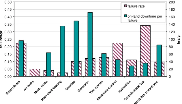
For this reason, the model has been applied first to a baseline case (for which failure rates and land-based down-times are shown in Figure 7) and then to a series of departures from it, a parameter set at a time, in order to explore how each set of parameters influences delay time and availability. The baseline case uses Windstats failure rate data from Germany as presented by Tavner [13], down-time figures from Durstewitz [10] and sea conditions and distance to shore as presented in Fugro [1] from a site 16km 062° (ENE) from North Somercotes in Lincs.

0.00 0.05 0.10 0.15 0.20 0.25 0.30 0.35 0.40 0.45 0.50

Rot or b

lade s

Air brak

e

Mec h. b

rake

Mai n sh

aft/b eari

ng

Gea rbox

Gen erat

or

Yaw sys

tem

Ele ctro

nic Con

trol

Hyd raul

ics

Grid /ele

ctri cal S

ys

Mec h/pi

tch cont

rol s ys.

fa

il

u

re

s

/y

r

0 20 40 60 80 100 120 140 160 180 200

h

rs

/y

r

failure rate

[image:8.595.141.457.389.569.2]

on-land downtime per failure

Figure 7: Baseline case failure rates & down-time per failure

All calculations were performed in a standard spreadsheet. (A small macro is required to calculate the incomplete gamma function, though there are routines and numerical recipes in the public domain). For any one fault class calculation, an appropriate threshold is set, the total offshore operation time is estimated from a travel time and a repair time and the

corresponding expected delay time is calculated. The expected annual delay caused by that fault class is the product of failure rate per year with the delay time per fault. The sum of all the subsystems’ annual contributions of down-time gives the total expected annual down-time and thereby the (un)availability.

4 Sample results & sensitivities

(9)

extent than might be guessed just from failure rates and repair times. Of course, these figures must be treated with caution but they illustrate the extent to which delays to repairs on large subsystems are exacerbated by the long operational time needed and the requirement for vessels that are over-sensitive to sea conditions.

0 100 200 300 400 500 600 700 800 900 1000

Rot or b

lade s

Air b rake

Mec h. b

rake

Mai n sh

aft/b eari

ng

Gea rbox

Gen erat

or

Yaw sys

tem

Ele ctro

nic Con

trol

Hyd raul

ics

Grid /ele

ctric al S

ys

Mec h/pi

tch cont

rol s ys.

h

rs

/y

r

[image:9.595.138.450.135.316.2]

repair time travel time delay time lead time

Figure 8: Expected annual contributions to downtime by subsystem

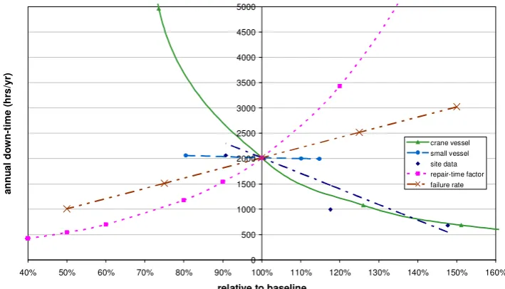
The effect of changing repair times was modelled by scaling the baseline case figures by factors between 40% and 160%. Similarly, failure rates were scaled by factors from 50% to 150%. The threshold wave heights for the 2 vessels examined were also varied relative to the baseline figure. Finally, site influence was modelled with actual site Weibull parameters. The percentage variation relative to baseline on the x-axis was based on the probability that the large vessel threshold wave height is exceeded.

It can be seen in Figure 9 that the threshold for the vessel required for small repairs has relatively little influence on annual down-time. The vessel for large repairs has the most influence. Repair time has somewhat more influence than failure rate.

0 500 1000 1500 2000 2500 3000 3500 4000 4500 5000

40% 50% 60% 70% 80% 90% 100% 110% 120% 130% 140% 150% 160%

relative to baseline

a

n

u

a

l

d

o

w

n

-t

im

e

(

h

rs

/y

r)

[image:9.595.120.475.469.672.2]

crane vessel small vessel site data repair-time factor failure rate

Figure 9: Sensitivity of turbine total annual expected down-time to different factors

5 Conclusions and further work

(10)

The current lack of data in the public domain regarding offshore wind farms prevents validation of the methodology and makes it hard to place confidence in absolute results of calculation though this would be equally true of other methods.

The advantage of the approach developed is that it does allow rapid investigation of the influence of various factors on downtime without having to run a long series of simulations for each new situation.

Calculations indicate that annual down-times may be dominated by repairs to the blades, generator and gearbox. These are not necessarily the subsystems with the highest failure rates but those requiring long repair windows and whose repairs currently require large crane vessels, the use of which is severely restricted by sea-state. The greatest influence on down-time and availability is found to come from changes in the access conditions for repairs, by reducing reliance on ‘sensitive’ vessels, by reducing repair time at the turbine and by reducing vessels’ sensitivity to sea-state. Repair times have more impact than failure rates. Access for the vessels used for small repairs seems to have little impact overall.

Future work would include the possibility of calculating confidence limits on results, standard deviations of expected delays, inclusion of other types of delays and more complex scenarios and extending the model to calculate costs and revenue losses.

6 References

1. Fugro GEOS. Wind and wave frequency distributions for sites around the British Isles. HSE Books, 2001, OTO report 01030.

2. Peters DJ, Shaw CJ, Grant CK, Heideman JC & Szabo D. Modelling the North Sea through the North European Storm Study. (NESS). Offshore Technology Conference, Report Number OTC 7130, p 479-493, 1993

3. http://www.cefas.co.uk/data/wavenet.aspx (Last accessed on 22/02/2008)

4. Offinger R. Maximum Likelihood and Least Squares Estimation in the Three-Parameter Weibull Model with Applications to River-Drain Data.

http://www.math.uni-magdeburg.de/~rooff/main.ps.gz (last accessed 12/08/2008), also:

http://citeseerx.ist.psu.edu/viewdoc/download?doi=10.1.1.29.6108&rep=rep1&type=url&i=0

(last accessed 20/08/2009)

5. Cran GW. Moment Estimators for the 3-Parameter Weibull Distribution. IEEE Trans on Reliability, Vol37, No4, 1988 Oct, pp360-363

6. Houmb OG & Vik I, On the duration of a Sea State, International Research Seminar on Safety of Structures under Dynamic Loading, Norwegian Institute of Technology,

Trondheim 1977, Vol 2 pp705-712 (Originally published in a fuller version as Report of Div. of Port and Ocean Engineering, Univ. of Trondheim, 1977)

7. Graham C, Parameterisation and prediction of wave height and wind speed

persistence statistics for oil industry operational planning purposes, Coastal Engineering 6,4 (1982) pp303-329

8. Mathiesen M, Estimation of wave height duration statistics, Coastal Engineering 23, 1-2 (1994) pp167-181

9. Kuwashima S & Hogben N, The estimation of wave height and wind speed

persistence statistics from cumulative probability distributions, Coastal Engineering 9,6 (1986) pp563-590, Elsevier, Amsterdam

10. Durstewitz M, Ensslin C, Hahn B, Rohrig K, +15 years practical experiences with wind power in Germany, EWEC 06

11. Ribrant J & Bertling LM, Survey of Failures in Wind Power Systems With Focus on Swedish Wind Power Plants During 1997–2005, IEEE Trans on Energy Conversion Vol 22 No 1 Mar 2007 pp167-173

12. Bussel GJW van & Zaaijer MB Estimation of Turbine Reliability figures within the DOWEC project, DOWEC Report Nr. 10048, Issue 4, 2002,

ftp://ftp.ecn.nl/pub/www/dowec/10048_004.pdf (last accessed 23/09/2009)