Exact potential and scattering amplitudes from the tachyon non-linear β-function

      

City, University of London Institutional Repository

Citation:

Coletti, E., Forini, V., Nardelli, G., Grignani, G. & Orselli, M. (2004). Exact potential and scattering amplitudes from the tachyon non-linear β-function. Journal of High Energy Physics, 2004, 030.. doi: 10.1088/1126-6708/2004/03/030

This is the published version of the paper.

This version of the publication may differ from the final published

version.

Permanent repository link:

http://openaccess.city.ac.uk/19747/

Link to published version:

http://dx.doi.org/10.1088/1126-6708/2004/03/030

Copyright and reuse: City Research Online aims to make research

outputs of City, University of London available to a wider audience.

Copyright and Moral Rights remain with the author(s) and/or copyright

holders. URLs from City Research Online may be freely distributed and

linked to.

City Research Online: http://openaccess.city.ac.uk/ [email protected]

Journal of High Energy Physics

Exact potential and scattering amplitudes from the

tachyon non-linear β-function

To cite this article: Erasmo Coletti et al JHEP03(2004)030

View the article online for updates and enhancements.

Related content

Boundary string field theory as a field theory—mass spectrum and interaction

Koji Hashimoto and Seiji Terashima

-Spectral flow and boundary string field theory for angledD-branes

Nicholas T. Jones and S.-H. Henry Tye

-Abelian and nonabelian vector field effective actions fromstring field theory

Erasmo Coletti, Ilya Sigalov and Washington Taylor

-Recent citations

Tachyon solutions in boundary and open string field theory

Gianluca Calcagni

-Nonlocal instantons and solitons in string models

Gianluca Calcagni and Giuseppe Nardelli

-Superstring disk amplitudes in a rolling tachyon background

-JHEP03(2004)030

Published by Institute of Physics Publishing for SISSA/ISAS Received:February 20, 2004

Accepted: March 10, 2004

Exact potential and scattering amplitudes from the

tachyon non-linear

β

-function

Erasmo Coletti

Center for Theoretical Physics, M.I.T. Cambridge, MA 02139, U.S.A.

E-mail: [email protected]

Valentina Forini and Giuseppe Nardelli

Dipartimento di Fisica and I.N.F.N. Gruppo Collegato di Trento, Universit`a di Trento 38050 Povo (Trento), Italia

E-mail: [email protected],[email protected]

Gianluca Grignani and Marta Orselli

Dipartimento di Fisica and Sezione I.N.F.N., Universit`a di Perugia Via A. Pascoli I-06123, Perugia, Italia

E-mail: [email protected],[email protected]

Abstract: We compute, on the disk, the non-linear tachyon β-function, βT, of the open bosonic string theory. βT _{is determined both in an expansion to the third power of the field}

and to all orders in derivatives and in an expansion to any power of the tachyon field in the leading order in derivatives. We construct the Witten-Shatashvili (WS) space-time effective action S and prove that it has a very simple universal form in terms of the renormalized tachyon field andβT_{. The expression forSis well suited to studying both processes that are}

far off-shell, such as tachyon condensation, and close to the mass-shell, such as perturbative on-shell amplitudes. We evaluate S in a small derivative expansion, providing the exact tachyon potential. The normalization ofS is fixed by requiring that the field redefinition that mapsS into the tachyon effective action derived from the cubic string field theory is regular on-shell. The normalization factor is in precise agreement with the one required for verifying all the conjectures on tachyon condensation. The coordinates in the space of couplings in which the tachyon β-function is non linear are the most appropriate to study RG fixed points that can be interpreted as solitons of S, i.e. D-branes.

JHEP03(2004)030

Contents

1. Introduction 1

2. Boundary string field theory 4

3. Integration over the bulk variables 6

4. Partition function on the disk and the renormalized tachyon field 7

5. Background-field method 11

6. β-function 13

7. Witten-Shatashvili action 17

8. Cubic vs. Witten-Shatashvili tachyon effective actions 22

9. Conclusions 24

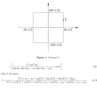
A. Computation of I(k1, k2, k3) 25

1. Introduction

One of the most interesting problems in string theory is to understand how the background space-time on which the string propagates arises in a self-consistent way. For open strings, there are two main approaches to this problem, cubic string field theory [1] and background independent string field theory [2]–[5].

Background independent open string field theory has been useful for finding the clas-sical tachyon potential energy functional and the leading derivative terms in the tachyon effective action [6]–[9]. It is formulated as a problem in boundary conformal field theory. One begins with the partition function of open-string theory where the world-sheet is a disk. The strings in the bulk are considered to be on-shell and a boundary interaction with arbitrary operators is added. The configuration space of open string field theory is then taken to be the space of all possible boundary operators modulo gauge transformations and field redefinitions. Renormalization fixed points, which correspond to conformal field theories, are solutions of classical equations of motion and should be viewed as the solutions of classical string field theory.

JHEP03(2004)030

of the decay are crucial questions. Some understanding of this process has been achieved for the open bosonic string. The key idea is that of Sen [10]. The open bosonic string tachyon reflects the instability of the D-25 brane. This unstable D-brane should decay by condensation of the open string tachyon field. The energy per unit volume released in the decay should be the D-25 brane tension and the end-point of the decay is the closed string vacuum [10, 11, 12, 7]. There are also intermediate unstable states which are the D-branes of all dimensions between zero and 25.

The decay of unstable systems of D-branes, pictured as a tachyon field rolling down a potential toward a stable minimum, can also be addressed in the context of the boundary string field theory. It involves deforming the world sheet conformal field theory of the unstable D-brane by an exact marginal, time dependent tachyon profile. The quantitative study of rolling tachyons was initiated by A. Sen [13]–[17] and has been recently used to obtain other forms of tachyon effective actions [18]–[22]. The construction of the space-time tachyon effective action in background independent open string field theory is the subject of the present paper.

By classical power-counting the tachyon field T(X) has dimension one and is a rel-evant operator. If T(X) is the only interaction, the field theory is perturbatively super-renormalizable. If T(X) and the other fields are adjusted so that the sigma model that they define is at an infrared fixed point of the renormalization group (RG), these back-ground fields are a solution of the classical equations of motion of string theory. Witten and Shatashvili [2, 4] have argued that these equations of motion come from an action which can be derived from the disk partition functionZby a prescription which we shall make use of below. According to this prescription the effective action for a generic coupling constant

gi _{(which can be identified with the tachyon, the gauge or any other field that correspond}

to excitations of the open bosonic string) is related to the renormalized partition function of open string theory on the disk,Z(gi), through

S =

µ

1₋βi δ δgi

¶

Z(gi), (1.1)

whereβi _{is the beta-function}1 _{of the coupling g}i_{. Note that (1.1) fixes the additive}

ambi-guity inS by requiring that at RG fixed points g∗_{, in which β}i_(g∗_{) = 0,}

S(g∗) =Z(g∗). (1.2) The derivative of the action S with respect to the coupling constant gi _{must be related to}

theβ-function through a metric according to

∂S ∂gi =−β

j_G

ij(g). (1.3)

Gijshould be a non-degenerate metric, otherwise there would be an extra zero which could

not be interpreted as a conformal field theory on the world sheet. Eq. (1.3) indicates that the RG flow is actually a gradient flow. The prescription (1.1) provides a definition of the metric Gij in the space of couplings.

1_{In this paper theβfunction is positive for relevant perturbations. In some other papers on the subject,}

JHEP03(2004)030

Theβ-functions appearing in (1.1) are in general non-linear functions of the couplings

gi_{. When the linear parts of the β}i _{(i.e. the anomalous dimensionsλ}

i of the corresponding

coupling) satisfy a so called “resonant condition”, the non linear parts of the β-function cannot be removed by a coordinate redefinition in the space of couplings [5]. Such resonant condition is nothing but the mass-shell condition so that, near the mass-shell, the β -functions are necessarily non-linear.

However, when the resonant condition does not hold, a possible choice of coordinates on the space of string fields is one in which theβ-functions are exactly linear. This choice can always be made locally [7] and is well suited to studying processes which are far off-shell, such as tachyon condensation. These coordinates, however, become singular when the components of the string field (e.g. T(X),Aµ(X) etc.) go on-shell. These coordinates

can be used to construct, for example, the tachyon effective potential, but become singular when one tries to derive an effective action which reproduces the on-shell amplitudes. In particular, if the Veneziano amplitude needs to emerge from the tachyon effective action it is necessary to consider the whole non-linearβ-function in (1.1). A complete renormalization of the theory in fact makes the β-function non-linear in T(X) [23] so that, since the vanishing of the β-function is the field equation for T, these nonlinear terms describe tachyon scattering. One of the goal of this paper is to construct non-linear expressions for theβ-functions which are valid away from the RG fixed point. With these expressions for the non-linear tachyon β-function we shall construct the Witten-Shatashvili (WS) space-time action (1.1). We shall prove that (1.1) has the following very simple form in the coupling space coordinates in which the tachyonβ-function is non-linear

S =K

Z

d26X£

1₋TR(X) +βT(X)

¤

, (1.4)

where TR is the renormalized tachyon field and K is a constant related to the D25-brane

tension. This formula is universal as it does not depend on how many couplings are switched on. Eq. (1.4) arises from the expression that links the renormalized tachyon field to the partition function that appears in (1.1), namelyZ =KR

d26X(1₋TR). TR is then

a non-linear function of the bare coupling T and in these coordinates the β-function is non-linear. When couplings other than the tachyon are introduced in Z, βT _{will depend}

on them so that S will provide the space-time effective action also for these couplings. With this prescription we shall compute the non-linearβ-function βT _{for the tachyon}

field up to the third order in powers of the field and to any order in derivatives of the field. From this we shall show that the solutions of the RG fixed point equations generate the three and four-point open bosonic string scattering amplitudes involving tachyons. Then, with the same renormalization prescription, we shall compute βT _{to the leading orders in}

derivatives but to any power of the tachyon field and we shall show thatS coincides with the one-found in [6, 7, 8]. Obviously,S up to the first three powers ofT and expanded to the leading order in powers of derivatives can be obtained from both calculations and the results coincide.

In the case of profilesTR(k) that have support near the on-shell momentumk2 '1 the

JHEP03(2004)030

that this action coincides with the tachyon effective action computed, for the almost on-shell profiles, form the cubic string field theory up to the fourth power of the tachyon field. The knowledge of the non-linear tachyonβ-function is very important also for another reason. The solutions of the equation βT _{= 0 give the conformal fixed points, the}

back-grounds that are consistent with the string dynamics. In the case of slowly varying tachyon profiles, we shall show that the equations of motion for the WS action can be made iden-tical to the RG fixed point equation βT _{= 0. We shall find solutions of this equation to}

which correspond a finite value of the WS action. Being solutions of the RG equations, these solitons are lower dimensional D-branes for which the finite value of S provides a quite accurate prediction of the D-brane tension.

We shall also show that the WS action constructed in terms of a linearβ-function [24] is related to the action (1.4) by a field redefinition, and that this field redefinition becomes singular on-shell. This is in agreement with the Poincar´e-Dulac theorem [25] used in [5] to prove that when the resonant condition holds, namely near the on-shellness, theβ-function has to be non-linear.

The tachyon effective action up to the third power in the fields is known exactly also from the cubic string field theory [1]. This raises the interesting question of how the action S obtained in this paper is related to the cubic SFT. It seems clear that the cubic SFT must correspond to (1.1), (1.3) for a particular choice of coordinates on the space of string fields (or worldsheet couplings). The two sets of coordinates are related by a complicated transformation which we shall derive in this paper. The cubic SFT parametrization of worldsheet RG is regular close to the mass shell. It very well reproduces tachyon scattering [26], to it must correspond a non-linear beta-function. Thus a coordinate transformation that relates the two effective actions needs a non-linear beta function in the definition (1.1). We shall show that this field redefinition exists and that it is non-singular on-shell only when K in (1.4) coincides with the tension of the D25-brane, in agreement with all the conjectures involving tachyon condensation [10, 27, 28].

2. Boundary string field theory

In Witten’s construction of open boundary string field theory [2] the space of all two dimensional worldsheet field theories on the unit disk, which are conformal in the interior of the disk but have arbitrary boundary interactions, is described by the world-sheet action

S =_S0+

Z 2π

0

dτ

2πV (2.1)

where_S0 is a free action describing an open plus closed conformal background and V is a

general perturbation defined on the disk boundary. We will discuss the twenty six dimen-sional bosonic string, for which (2.1) can be expressed in terms of a derivative expansion (or level expansion) of the form

V =T(X) +iAµ(X)∂τXµ+Bµν(X)∂τXµ∂τXν +Cµ(X)∂τ2Xµ+· · ·. (2.2)

Without the perturbation _V the boundary conditions on X are ∂rXµ|r=1 = 0, wherer is

JHEP03(2004)030

V is a ghost number zero operator and it is useful to introduce a ghost number one

operator _O via

V=b−1O. (2.3)

We shall consider the simplest case in which ghosts decouple from matter so that, as in (2.2), _V is constructed out of matter fields alone

O=c_V. (2.4)

The space-time string field theory action S is defined through its derivative dS which is a two point function computed with the worldsheet action (2.1). More generally one can introduce some basis elements _Vi for operators of ghost number 0 so that the space of

boundary perturbations_V can be parametrized as

V =X

i

gi_Vi (2.5)

where the coefficients gi _{are couplings on the world-sheet theory, which are regarded as}

fields from the space-time point of view, and _O = P

igiOi. In this parametrization the

space-time action is defined through its derivatives with respect to the couplings and has the form

∂S ∂gi =

K

2

Z 2π

0

dτ

2π

Z 2π

0

dτ0

2πhOi(τ){Q,O(τ

0_)}i

g, (2.6)

whereQis the BRST charge and the correlator is evaluated with the full perturbed world-sheet action _S.

If_Vi is a conformal primary field of dimension ∆i, for O’s of the form (2.4), one has

{Q, c_Vi}= (1−∆i)c∂τcVi, (2.7)

so that from (2.6) one gets

∂S

∂gi =−(1−∆j)g j_G

ij(g), (2.8)

where

Gij= 2K

Z 2π

0

dτ

2π

Z 2π

0

dτ0

2π sin

2

µ

τ ₋τ0

2

¶

hVi(τ)Vj(τ0)ig. (2.9)

Eq. (2.8) cannot be true in general, since it does not transform covariantly under reparame-trizations of the space of theories, gj _→fj_(gi_{). Indeed,∂}

iS andGij transform as tensors,

(the latter is the metric on the space of worldsheet theories), but gi _{does not.}

The correct covariant generalization of (2.8) was given in [4, 5]. The worldsheet RG defines a natural vector field on the space of theories: the β-function βi_{(g), which}

trans-forms as a covariant vector under reparametrizations of gi_{. The covariant form of (2.8)}

is thus (1.3). If we assume that total derivatives inside the correlation function decouple and that there are no contact terms, it turns out that theβ-function in (1.1) is the linear

JHEP03(2004)030

on the world-sheet and cannot be ignored. The point is that the operatorQ, which is con-structed out of the BRST operator in the bulk and should be independent on the couplings because the perturbation is on the boundary, actually depends on the couplings when the contour integral approaches the boundary of the disk. A way to fix the structure of the contact terms is to consider that, since dS is a one-form, the derivative of dS should be zero independently of the choice of the contact terms that one makes in the computation. This leads to the following formula for the vector field in equation (1.1)

βi = (1₋∆i)gi+αijkgjgk+γjkli gjgkgl+· · · . (2.10)

This is an expression for the β-function with all the non-linear terms. According to the Poincare-Dulac Theorem about vector fields (whose relevance to the β-function related issues was stressed many times by Zamolodchikov [25]) every vector field can be linearized by an appropriate redefinition of the coordinates up to the resonant term. In the second order of equation (2.10) the resonance condition is given by

∆j + ∆k−∆i= 1. (2.11)

The resonance condition means that the β-function cannot be linearized by a coordinate transformation and that all the non-linear terms cannot be removed from the β-function equation (2.10). When gi is the tachyon field T(k), the resonant condition (2.11) corre-sponds to the mass-shell conditions for three tachyons. We shall prove in what follows that the WS action S up to the third order in the tachyon fields, constructed in terms of the linear β-function [24], is related to the S made of a non-linear β-function by a field redefinition, but that this field redefinition becomes singular on-shell.

3. Integration over the bulk variables

Let us now restrict ourselves to the specific example of open strings propagating in a tachyon background. The partition function reads

Z =

Z

[dXµ(σ, τ)] exp (₋S[X]), (3.1)

where the action is

S[X] =

Z

dσdτ 1

4π∂aX(σ, τ)·∂aX(σ, τ) +

Z 2π

0

dτ

2πT(X(τ)). (3.2)

Here, the first term in (3.2) is the bulk action and is integrated over the volume of the unit disk. The second term in (3.2) is integrated on the circle which is the boundary of the unit disk and describes the interactions. The scalar fieldsXµ _{haveD components with}

µ = 1, . . . , D and we shall assume D = 26 in what follows for a critical string. We are

working in a system of units whereα0 _{= 1.}

We begin with the observation that the bulk excitations can be integrated out of (3.1) to get an effective non-local field theory which lives on the boundary [29]. To do this we write the field in the bulk as [9]

JHEP03(2004)030

where

∂2Xcl= 0

and Xcl approaches the fixed (for now) boundary value ofX,

Xcl →Xbdry andXqu→0.

Then, in the bulk, the functional measure is dX=dXqu and

S =

Z

d2σ

4π ∂Xqu·∂Xqu+

Z

dτ

2π

½

1 2X

µ

|i∂τ|Xµ+T(X)

¾

, (3.3)

where we omitted the cl index in the last integral. Then, the integration of Xqu produces

a multiplicative constant in the partition function - the partition function of the Dirichlet string, which we shall denote K. The kinetic term in the boundary action is non-local. The absolute value of the derivative operator is defined by the Fourier transform,

|i∂τ|δ(τ −τ0) =

X

n |n_|

2πe

in(τ−τ0₎

.

The partition function of the boundary theory is then

Z(J) =K

Z

[dXµ]e− R2π

0

dτ

2π(

1 2X

µ_|i∂|Xµ_{+T(X)−J·X)}

, (3.4)

where we have added a sourceJµ(τ) so that the path integral can be used as a generating functional for correlators of the fields Xµ _{restricted to the boundary. In particular, this}

source will allow us to compute the correlation functions of vertex operators of open string degrees of freedom. The remaining path integral over the boundaryXµ_{(τ) defines a}

one-dimensional field theory with non-local kinetic term. If the tachyon field were absent (T = 0), the further integration overXµ_{(τ) would give a factor which converts the Dirichlet}

string partition function to the Neumann string partition function.

4. Partition function on the disk and the renormalized tachyon field

When only the tachyon field is considered as a boundary perturbation, the Witten-Shatash-vili action is given by

S =

µ

1₋

Z

βT δ δT

¶

Z , (4.1)

whereZ is the partition function of the boundary theory on the disk andβT is the tachyon

β-function. It is useful to introduce a constant source term k for the zero mode of the

X field, the integral over the zero mode variable will just provide the energy-momentum conservationδ-function. The partition function (3.4) in the presence of this constant source reads

Z(k) =K

Z

[dXµ]e− R2π

0

dτ

2π(

1 2X

µ_|i∂

JHEP03(2004)030

where ˆX is the zero mode which is defined by

ˆ

Xµ=

Z 2π

0

dτ

2πX

µ_{(τ). (4.3)}

In this section we shall expand the exponential in eq. (4.2) in powers of T(X). The first non-trivial term is

Z(1)(k) =₋K

Z

[dXµ]

Z

dk1

Z 2π

0

dτ1

2πT(k1)e

−R2π

0

dτ

2π(

1 2X

µ_|i∂

τ|Xµ)−ikXˆ+ik1X(τ1)_{. (4.4)}

The functional integral over the non-zero modes ofX(τ) gives

Z(1)(k) =₋K

Z

dXˆµ

Z

dk1T(k1)e−

k₁2

2 G(0)+i(k1−k) ˆX, (4.5)

whereG(τ) is the Green function of the operator _|i∂τ|

G(τ1−τ2) = 2 ∞

X

n=1

e−²ncosn(τ1−τ2)

n =−log

£

1₋2e−²cos (τ1−τ2) +e−2²

¤

(4.6)

and ²is a cut-off. In all the calculations we shall use the following prescription forG(τ)

G(τ) =

(

−loghcsin2³τ 2

´i

τ ₆= 0

−2 log² τ = 0 . (4.7) The coefficient c reflects the ambiguity involved in subtracting the divergent terms. Its value is scheme dependent and should be fixed by some renormalization prescription. We choose the valuec= 4 for later convenience. This arbitrariness was discussed in [8, 9]. The integrals over the zero-modes in eq. (4.5) give a 26-dimensional δ-function so that

−Z(1)(k) =KT(k)²k2−1 (4.8)

and we can identify

TR(k)≡T(k)²k

2₋₁

=₋Z

(1)_(k)

K . (4.9)

This equation provides the renormalized coupling TR in terms of the bare coupling T to

the lowest order in perturbation theory. 1₋k2 _{is the anomalous dimension of the tachyon}

field. The second order term in T is given by

Z(2)(k) =K

Z 2π

0 dτ1 4π dτ2 2π Z

dk1dk2T(k1)T(k2)

D

eik1X(τ1)_eik2X(τ2)_e−ikXˆ

E

. (4.10)

Again in (4.10) the integral over the zero modes ˆXµ_{gives just a 26-dimensionalδ-function,}

δ(k₋k1−k2), and we can perform the integral over the non-zero modes ofX(τ) to get

Z(2)(k) = K

Z 2π

0 dτ1 4π dτ2 2π Z

dk1dk2(2π)Dδ(k−k1−k2)T(k1)T(k2)×

×exp

·

−1₂¡

k₁2+k₂2¢

G(0)₋k1k2G(τ1−τ2)

¸

JHEP03(2004)030

The integral in (4.11) becomes

Z(2)(k) = K

Z

dk1dk2(2π)Dδ(k−k1−k2)²k 2

1+k22−2T(k

1)T(k2)×

×

Z 2π

0 dτ1 4π dτ2 2π ·

4 sin2

µ

τ1−τ2

2

¶¸k1k2

. (4.12)

The integral over the relative variable x = (τ1 −τ2)/2 does not need regularization, it

converges when 1 + 2k1k2>0, providing the result

Z(2)(k) = K 2

Z

dk1dk2(2π)Dδ(k−k1−k2)²k 2

1+k22−2T(k

1)T(k2)

Γ(1 + 2k1k2)

Γ2_{(1 +k} 1k2)

. (4.13)

The integrand in (4.13) can be analytically continued also to the region where 1+2k1k2 <0,

so that the integral can be performed.

To the second order in perturbation theory the renormalized coupling in terms of the bare coupling reads

TR(k) = −

Z(1)_{(k) +Z}(2)_(k)

K

= ²k2−1

·

T(k)₋1 2

Z

dk1dk2(2π)Dδ(k−k1−k2)×

×T(k1)T(k2)²−(1+2k1k2)

Γ (1 + 2k1k2)

Γ2_{(1 +k} 1k2)

¸

. (4.14)

The third order contribution to the partition function is given by

Z(3)(k) =₋K 3!

Z

dk1dk2dk3(2π)Dδ

à k₋ 3 X i=1 ki !

²P3i=1k 2

i−3T(k₁)T(k₂)T(k₃)I(k₁, k₂, k₃),

(4.15) whereI(k1, k2, k3) is the integral

I(k1, k2, k3) =

22k1k2+2k2k3+2k1k3

(2π)3

Z 2π

0

dτ1dτ2dτ3

·

sin2

µ

τ1−τ2

2

¶¸k1k2

×

×

·

sin2

µ

τ2−τ3

2

¶¸k2k3·

sin2

µ

τ1−τ3

2

¶¸k1k3

. (4.16)

The complete computation ofI(k1, k2, k3) will be given in appendix A. The result is given

by the completely symmetric formula

I(a1, a2, a3) =

Γ(1 +a1+a2+a3)Γ(1 + 2a1)Γ(1 + 2a2)Γ(1 + 2a3)

Γ(1 +a1)Γ(1 +a2)Γ(1 +a3)Γ(1 +a1+a2)Γ(1 +a2+a3)Γ(1 +a1+a3)

,

(4.17) where we have set a1 = k1k2, a2 = k2k3 and a3 = k1k3. The integral (4.16) converges

when 1 +a1+a2+a3 >0, but its result (4.17) can be analytically continued also outside

JHEP03(2004)030

ref. [7]. Up to the third order in powers of T and to all orders in ki the relation between

the bare and the renormalized couplings reads

TR(k) = −

Z(1)_{(k) +Z}(2)_{(k) +Z}(3)_(k)

K

= ²k2−1

"

T(k)₋1 2

Z

dk1dk2(2π)Dδ

à k₋ 3 X i=1 ki !

T(k1)T(k2)²−(1+2k1k2)×

×Γ (1 + 2_{Γ2(1 +}k_k1k2) 1k2)

+

Z

dk1dk2dk3

(2π)D

3! δ Ã k₋ 3 X i=1 ki ! ×

×T(k1)T(k2)T(k3)²−2(1+

P

i<jkikj)_I(k

1, k2, k3)

#

. (4.18)

In section 6 we shall use this expression to construct the non-linear β-function.

The renormalized tachyon field can be constructed to all powers of the bare tachyon field in the case in which the tachyon profile appearing in (4.2) is a slowly varying function ofXµ_{. In this case one can consider an expansion of (4.2) in powers of derivatives ofT. To}

this purpose consider then-th term in the expansion of (4.2) in powers ofT(X(τ)),Z(n)(k). Taking the Fourier transform of the tachyon field and performing all the contractions of theX(τi) fields, forZ(n)(k) we get

Z(n)(k) = K(−1)

n

n! ²

−n

Z n Y

i=1

dkiT(ki)

Z 2π

0 n Y i=1 µ dτi 2π ¶ ×

×e−Pni=1

k2_i

2 G(0)−

P

i<jkikjG(τi−τj)_δ

à k₋ n X i=1 ki ! . (4.19)

Note that with our regularization prescription the dependence on the cut-off in (4.19) comes only from the zero distance propagatorG(0) and from the explicit scale dependence of the tachyon field. If the tachyon profile is a slowly varying function ofXµ_{we can expand inside}

the integrand of (4.19) in powers of the momentaki. The leading and next to leading terms

in this expansion read

Z(n)(k) = K(−1)

n n! n Y i=1 Z

dkiδ

à k₋ n X i=1 ki !

²−n

n

Y

i=1

T(ki)×

×

 1 +

n

X

i=1

ki2log²+

X

i<j

kikjlog

c

4



, (4.20)

where the last term comes from the integral over a couple ofτ variables of the propagator

G(τi−τj), the other integrations overτk k 6=i, j being trivial. Here we have kept explicit

the ambiguitycappearing in the propagator (4.7) to show that the result greatly simplifies with the choice c = 4. Unless otherwise stated, we shall adopt this choice throughout the paper. As before, the renormalized tachyon field TR(k) can be obtained from (4.20)

JHEP03(2004)030

transform of TR(k) with c = 4, to all orders in the bare tachyon field and to the leading

order in derivatives, we get the renormalized tachyon fieldTR(X)

TR(X) = 1−exp

½

−1_²[T(X)_{− 4}T(X) log²]

¾

(4.21)

where ₄is the laplacian. Again in section 6 we shall use this expression to compute the non-linear tachyon β-function.

From eqs. (4.9), (4.14), (4.18), (4.21) it is clear that the general relation between the renormalized tachyon fieldTR(X) and the partition function Z≡Z(k = 0) is simply

Z =K

Z

d26X[1₋TR(X)]. (4.22)

This expression is true also when other couplings are present. TR in this case would be

a non linear function also of the other bare couplings but its relation with the partition function of the theory would always be given by (4.22). We shall prove eq. (4.22) in the next section.

5. Background-field method

The partition function of the boundary theory on the disk in general is given by

Z =K

Z

[dXµ]e−(S0[X]+ R2π

0

dτ

2πV[X(τ)]), (5.1)

where S0 =

R

dτ Xµ_|i∂

τ|Xµ and V[X(τ)] is given in (2.2). Our goal is to determine the

relationship between the renormalized and the bare couplings of the one-dimensional field theory. To this purpose we shall make use of the background field method [23]. We expand the fields Xµ _{around a classical background X}µ

0 which satisfies the equations of motion

and which varies slowly compared to the cut-off scale,

Xµ=X₀µ+Yµ.

The effective action is Seff[X0] = −logZ[X0] and the aim of the renormalization process

is to rewrite the local terms of Seff[X0] in terms of renormalized couplings in such a way

thatSeff[X0] has the same form of the original action

Seff[X0]

¯ ¯ ¯ ¯

local

=S0[X0] +

Z 2π

0

dτ

2πVR[X0(τ)]. (5.2)

Z[X0] can be conveniently calculated in powers of the boundary interaction V. The first

order for example reads, up to the multiplicative constant K,

−

Z 2π

0

dτ

2π

Z

dkeikX0_{h[T(k) +iA}

µ(k)∂τ(X₀µ+Yµ) +Bµν(k)∂τ(X₀µ+Yµ)∂τ(X0ν+Yν) +

+Cµ(k)∂τ2(X µ

JHEP03(2004)030

The renormalized couplings TR(k) will be given by the opposite of the coefficient of the

term in (5.3) that does not contain X0 derivatives. Analogously, the renormalized ARµ(k)

will be determined by the coefficient of ∂τX0µ, BµνR(k) by the coefficient of∂τX0µ∂τX0ν and

so on. The second order term in the expansion of Z[X0] is

Z 2π

0

dτ1

2π

Z 2π

0

dτ2

4π

Z

dk1dk2eik1X0(τ1)+ik2X0(τ2)×

×heik1Y(τ1)+ik2Y(τ2)_[T(k

1) +iAµ(k1)∂τ1(X

µ

0 +Yµ) +. . .]× ×[T(k2) +iAν(k2)∂τ2(X

ν

0 +Yν) +. . .]i. (5.4)

An expansion of the background fieldX0in powers of its derivatives is required to determine

the coefficients of 1, ∂τX₀µ, ∂τX₀µ∂τX₀ν, . . . ,

X0(τ2) =X0(τ1) + (τ2−τ1)∂τ1X0(τ1) +· · · . (5.5)

If we are interested in renormalization of couplings of the form exp[ikX0], namely in the

renormalized tachyon field TR(k), we can disregard the terms in (5.5), (5.4) involving

derivatives acting on X0. For example, at the second order, the only non-vanishing terms

inT and Aµ contributing to TR are

TR(k) = −

Z

dk1

Z

dk2δ(k−k1−k2)

Z 2π

0

dτ2

4π ×

×heik1Y(τ1)+ik2Y(τ2)_[T(k

1)T(k2) +Aµ(k1)Aν(k2)∂τ1Y

µ_∂ τ2Y

ν ₊

· · ·]_i, (5.6)

where the correlator does not depend on τ1 since the propagator (4.7) of X(τ) and its

derivatives are periodic functions on the unit circle. It is not difficult to see that TR(k)

in (5.6) coincides with the opposite of the second order term in the expansion of the partition function

Z(k) =

Z

[dYµ]e−(S0[Y]+ R2π

0

dτ

2πV[Y(τ)])−ikYˆ (5.7)

in powers of the couplings. Here k is a constant source for the zero mode of the Yµ field, ˆ

Yµ _{(4.3). Such a constant source will just provide the δ-function in (5.6) that imposes}

the energy-momentum conservation. This will be true at any order in the expansion in powers of the coupling fields. Therefore, to all orders in whatever coupling, the expression for the renormalized tachyon fieldTR(X) is related to the partition functionZ =Z(k= 0)

precisely by (4.22), which is the relation that we wanted to prove. Note that TR depends

not only on the bare tachyon field but also on the other coupling fields (in particular TR

will exists also if one starts from a boundary interaction that does not contain the bare tachyon). As a consequence, the tachyonβfunction will contain for example also the gauge field [30], and this is as it should be, since the solution of the equation βT _{= 0 will then}

JHEP03(2004)030

6. β-function

In this section we shall perform a calculation of the non-linear tachyon β-function. The resulting expression will then be used to derive the Witten-Shatashvili action (1.4), (4.1). Following [23], the most general RG equations for a set of couplings gi _{can be written as}

βi_≡ dg

i

dt =λig

i_+αi

jkgjgk+γjkli gjgkgl+· · · , (6.1)

where the scale t is t = ₋log², λi are the anomalous dimensions corresponding to the

couplings gi and there is no summation in the first term on the right-hand side. This equation has the solution

gi(t) =eλit_gi_{(0) +}h_e(λj+λk)t_−eλiti α

i jk

λj+λk−λi

gj(0)gk(0) +bi_jkl(t)gj(0)gk(0)gl(0) +_{· · ·} ,

(6.2) wheregi_{(0) are the bare couplings and}

bi_jkl(t)gj(0)gk(0)gl(0) =

"

µ _2αi

jmαmkl

λj +λm−λi −

γ_jkli

¶

eλit λj+λk+λl−λi

+

+

µ _2αi

jmαmkl

λk+λl−λm

+γ_jkli

¶

e(λj+λk+λl)t λj+λk+λl−λi −

− 2α

i jmαmkl

(λj+λm−λi) (λk+λl−λm)

e(λj+λk)t

#

gj(0)gk(0)gl(0).(6.3)

Let us now consider the case of interest for this paper: open strings propagating in a tachyon background. In this case the coupling gi is the tachyon field T(k). Thenλi = 1−k2 and

λj = 1−k2j. Comparing the general solution (6.2) with eq. (4.18) derived in the previous

section, we will be able to identify the renormalized tachyon field in terms of the bare field up to the third order in powers of the field and to all orders in its derivatives. In the second order term of (4.18) the coefficient proportional toeλit _=²1−k2 _{appearing in (6.1) is absent.}

This is due to the fact that the convergence condition for the integral (4.12), 1 + 2k1k2 >0,

implies thatλj+λk> λiso that in the limitt→ ∞the dominant contribution comes from

e(λj+λk)t_{. From similar arguments, the first and the second terms of the right-hand side}

of (6.3) are negligible compared to the second term, due to the convergence conditions for the integralI(k1, k2, k3) computed in the previous section. This is a general feature of our

renormalization procedure. At the n-th order in the bare coupling in the expansion (6.2), the renormalized coupling will contain only the term of the form

etPnk=1λk_{. (6.4)}

This is due to the fact that the integrals over the τ’s do not need an explicit regulator, rather they can be evaluated in a specific region of theki variables and then analytically

JHEP03(2004)030

Comparing our result for the renormalized tachyon field (4.18) with the general ex-pressions (6.2), (6.3), for the coefficients in the expansion (6.1) we find

αi_jk = ₋1 2

Γ(2 + 2kjkk)

Γ2_{(1 +kjkk)}δ(k−kj −kk)

γi jkl =

1 3!

Z

dkjdkkdklδ(k−kj−kk−kl)

×

·

2(1 +kjkk+kjkl+kkkl)I(kj, kk, kl)−

−

µ

Γ(2 + 2kjkk+ 2kjkl)Γ(1 + 2kkkl)

Γ2_{(1 +k}

jkk+kjkl)Γ2(1 +kkkl)

+ cycl.

¶ ¸

, (6.5)

where I(kj, kk, kl) is given in equation (4.17). The perturbative expression for the β

-function up to the third order in the tachyon field obtained using this procedure therefore is

βT(k) = (1₋k2)TR(k)−

1 2

Z

dk1dk2(2π)Dδ(k−k1−k2)TR(k1)TR(k2)

Γ(2 + 2k1k2)

Γ2_{(1 +k} 1k2)

+

+1 3!

Z

dk1dk2dk3(2π)Dδ(k−k1−k2−k3)TR(k1)TR(k2)TR(k3)×

×

·

2(1 +k1k2+k1k3+k2k3)I(k1, k2, k3)−

−

µ

Γ(2 + 2k1k2+ 2k1k3)Γ(1 + 2k2k3)

Γ2_{(1 +k}

1k2+k1k3)Γ2(1 +k2k3)

+ cycl.

¶ ¸

. (6.6)

We have thus succeeded in deriving a β-function for tachyon backgrounds which do not satisfy the linearized on-shell condition. Exactly the same result can be obtained by taking the derivative of (4.18) (or of the opposite of Z(k)) with respect to the logarithm of the cut-off ₋log². The result obtained in this way must then be expressed in terms of the renormalized field by inverting (4.18) and it coincides with (6.6).

It is interesting to note that all the known conformal tachyon profiles, like eiX0

or cosXi _{where iis a space index, are solutions of the equation β}T_{(X) = 0, whereβ}T_{(X) is}

the Fourier transform of (6.6). These solutions and perturbations around them have been recently used to construct tachyon effective actions around the on-shellness [31, 18, 19, 20, 22] and to study the problem of the rolling tachyon [13, 14, 15, 16, 17, 32, 21].

That the non-linear β-function (6.6) is the correct one can be shown by solving the

βT_{(k) = 0 equation perturbatively. The solution of this equation will generate the correct}

scattering amplitudes of open string theory [23]. This in turn will show the validity of the general formula (4.22). To the lowest order the equation is (1₋k2)T0(k) = 0, so that the

solution T0(k) satisfies the linearized on-shell condition. By writing T(k) =T0(k) +T1(k)

and substituting into the equation βT(k) = 0, to the next order we find

T1(k) = 1

2

Z

dk1dk2(2π)Dδ(k−k1−k2)T0(k1)T0(k2) Γ(k 2₎

(1₋k2_{) Γ}2_(k2_/2) . (6.7)

The presence of the couplings T0 in (6.7) sets two of the three ki on-shell. To pick out

JHEP03(2004)030

The calculation at the next order proceed in a similar fashion. One sets T(k) =

T0(k) +T1(k) +T2(k) and finds

T2(k) = −

(2π)D

3!(1₋k2₎

Z

dk1dk2dk3δ(k−k1−k2−k3)T0(k1)T0(k2)T0(k3)I(k1, k2, k3)×

×

(

2

Ã

1 +X

i<j

kikj

!

I(k1, k2, k3)−

·

Γ(2 + 2k1k2+ 2k1k3)Γ(1 + 2k2k3)

Γ2_{(1 +k}

1k2+k1k3)Γ2(1 +k2k3)

+ cycl.

¸

−

−

·

Γ(2 + 2k1k2+ 2k1k3)Γ(2 + 2k2k3)

Γ2_{(1 +k}

1k2+k1k3)Γ2(1 +k2k3)[1−(k2+k3)2]

+ cycl.

¸)

. (6.8)

When all the tachyons are on-shell, the last two terms on eq. (6.8) cancel and, as it should be for consistency, the residue of the pole ink is the scattering amplitude of four on-shell tachyons. It is given by

Γ(1 + 2k1k2)Γ(1 + 2k2k3)Γ(1 + 2k1k3)

Γ(1+k1k2)Γ(1+k2k3)Γ(1+k1k3)Γ(1+k1k2+k2k3)Γ(1+k2k3+k1k3)Γ(1+k1k2+k1k3)

,

(6.9) where the on-shell condition is 1 +k1k2 +k2k3 +k1k3 = 0. By means of the on-shell

condition, from the above expression, we recover, up to a normalization constant, the Veneziano amplitude, the scattering amplitude of four on-shell tachyons. Eq. (6.9) in fact becomes

1

π3Γ(1 + 2k1k2)Γ(1 + 2k2k3)Γ(1 + 2k1k3) sin(πk1k2) sin(πk2k3) sin(πk1k3) =

= 1

(2π)2 [B(1 + 2k1k2,1 + 2k2k3) + cycl.], (6.10)

where B(x, y) is the Euler beta function. The expression between square brackets is just the Veneziano amplitude. The ambiguitycappearing in the propagator (4.7) could be kept undetermined throughout the calculations of the scattering amplitudes. It is not difficult to see that this would just consistently change the normalization of the on-shell amplitudes.

For tachyon profilesTR(k) supported over near on-shell momentumk2'1, the

equa-tion of moequa-tion βT _{= 0 withβ}T _{given in (6.6) becomes}

βT(k) = (1₋k2)TR(k)−

(2π)D 2π

Z

dk1dk2δ(k−k1−k2)TR(k1)TR(k2)+

+ (2π)

D

3!(2π)2

Z

dk1dk2dk3δ(k−k1−k2−k3)TR(k1)TR(k2)TR(k3)× (6.11) ×{[B(1 + 2k1k2,1 + 2k2k3) + cycl.] + 2πtan(πk1k2) tan(πk1k3) tan(πk2k3)}= 0.

The coefficients of the quadratic and cubic terms in (6.11) are symmetric with respect to all the ki and k when these are on the mass-shell. Thus (6.11) can be derived as the

JHEP03(2004)030

amplitude with great accuracy already at levelL= 50. The tachyon effective action arising from the cubic string field theory for near on shell tachyon profiles Φ(k) therefore reads2

SC = 2π2T25(2π)D

(

−1₂

Z

dkΦ(k)Φ(₋k)(1₋k2) +1 3

Z 3 Y

i=1

dkiΦ(ki)δ

µ 3 X

i=1

ki

!

+

+ 1 4!

Z 4 Y

i=1

dkiΦ(ki)δ

à ₄ X

i=1

ki

!

[B(1+2k1k2,1+2k2k3) + cycl.]

)

, (6.12)

where the tachyon momenta in the fourth order term satisfy

k1 = (0,1,0,0, . . . ,0) k2= (0,sinθ,cosθ,0, . . . ,0) (6.13)

k3 = (0,−1,0,0, . . . ,0) k4 = (0,−sinθ,−cosθ,0, . . . ,0). (6.14)

Since the Veneziano amplitude is completely symmetric in the four momenta ki, it is not

difficult to see that the equation of motion deriving from (6.12) becomes precisely (6.11) once the simple field rescaling T = 2πΦ is performed. Thus the cubic string field theory for almost on-shell tachyons reproduces the non-linearβT _{= 0 equation of motion.}

In section 4 we also derived the renormalized tachyon field for the case of a slowly varying tachyon profile, to all orders in the bare field and to the leading order in derivatives, eq. (4.21). From this we can easily compute the corresponding β function. The task in this case is much simpler, as we just need to take the derivative of (4.21) with respect to

−log²

β(X) = ∂TR(X)

∂(₋log²) = 1

²exp

µ

−T(_²X)

¶ ½

T(X) +₄T(X)

·

1₋

µ

1₋T(X)

²

¶

log²

¸¾

.

(6.15) Then we have to invert the relation (4.21) between TR and T. To the leading order in

derivatives one has

T(X) =₋²_{[1 + (log²)₄] log(1₋TR(X))}, (6.16)

from which it is clear that the admissible range for TR is −∞ ≤TR≤1. Plugging (6.16)

into (6.15) we get the non-linear tachyon β-function to all powers of the renormalized tachyon and to the leading order in its derivatives

βT(X) = (1₋TR(X)) [−log (1−TR(X))− 4log (1−TR(X))]. (6.17)

βT_{(X) = 0 is the tachyon equation of motion for a slowly varying tachyon profile.}

Since in our calculations of the non-linear β-function we have always used the same coordinates in the space of string fields, the two results (6.17) and (6.6) should coincide when expanded up to the third power of the field and to the leading order in derivatives, respectively. This is indeed the case and the result in both cases reads

βT(X) =₄TR+∂µTR∂µTR+TR∂µTR∂µTR. (6.18)

2_{Here we include also the contribution due to the tachyon field in the quartic term so that this on-shell}

JHEP03(2004)030

It is interesting to compute the β-function also in the case in which the ambiguity constantcappearing in (4.7) is kept undetermined. TR(k) can be easily obtained as before

from (4.20) without fixing c = 4. By taking the Fourier transform and by differentiating with respect to₋log², theβ-function expressed in terms of the renormalized tachyon field

TR(X) turns out to be

βT(X) = (1₋TR)

·

−log (1₋TR) + 4

TR

1₋TR

+

µ

1 + 1 2log

c

4

¶

∂µTR∂µTR

(1₋TR)2

¸

. (6.19)

In the next section we shall use also this form of the β-function to construct the Witten-Shatashvili action.

7. Witten-Shatashvili action

In this section we shall compute the Witten-Shatashvili action. From the simple expression that relates the partition function to the renormalized tachyon (4.22) it is easy to deduce a simple and universal form for the WS action of the open bosonic string theory

S =

µ

1₋

Z

βT δ

δTR

¶

Z[TR] =K

Z

dDX£

1₋TR(X) +βT(X)

¤

. (7.1)

This can now be computed in both the cases analyzed in the previous sections. We shall show that the expressions for S that we will obtain are consistent both with the known results on the tachyon potential [7] and with the expected on-shell behavior. Thus a choice of coordinates in the space of couplings in which the tachyonβ-function is non-linear allows one to find not only a simple general formula for the WS action, but provides also a space-time tachyon effective action that describes tachyon physics from the far-off shell to the near on-shell regions.

Let us start with the evaluation of (7.1) up to the third order in the expansion of the tachyon field using the non-linear β-function (6.6). A similar computation was done in [7, 24] by means of the linear β-function, β(k) =¡

1₋k2¢

T(k). We shall later compare the two results. From the renormalized field (4.18) and the β-function (6.6) we arrive at the following expression for the Witten action

S = K

(

1₋1 2

Z

dk(2π)DTR(k)TR(−k)

Γ(2₋2k2₎

Γ2_(1−k2₎ +

+ 1 3!

Z

dk1dk2dk3(2π)DTR(k1)TR(k2)TR(k3)δ(k1+k2+k3)× (7.2)

×

"

2

Ã

1+X

i<j

kikj

!

I(k1, k2, k3)−

µ

Γ(1 + 2k2k3)Γ(2 + 2k1k2+ 2k1k3)

Γ2_{(1 +k}

2k3)Γ2(1 +k1k2+k1k3)

+cycl.

¶#)

.

The propagator coming from the quadratic term in (7.2) exhibits the required pole at

JHEP03(2004)030

show that these are due to the metric in the coupling space appearing in (1.3). The equations of motion derived from the action (7.2) are

δS δTR(−k)

= ₋KΓ(2−2k

2₎

Γ2_(1−k2₎(2π)

D_{T(k) +}K

2

Z

dk1dk0(2π)Dδ(k1+k0−k)TR(k1)TR(k0)×

×

½

2(1₋k1k+k1k0−kk0)I(−k, k1, k0)−

Γ(1₋2kk1)Γ(2−2kk0 + 2k1k0)

Γ2_(1−kk

1)Γ2(1−kk0+k0k1) − −Γ(1−2kk

0_)Γ(2−2kk

1+ 2k0k1)

Γ2_(1−kk0_)Γ2_(1−kk

1+k0k1) −

Γ(1 + 2k0k1)Γ(2−2kk0−2kk1)

Γ2_{(1 +k}0_k

1)Γ2(1−kk0−kk1)

¾

.

(7.3) As we did for the equation βT _{= 0 in the previous section, by solving these equations}

perturbatively it is possible to recover the scattering amplitudes for three on-shell tachyons. To the lowest order the equation is

Γ(2₋2k2)

Γ2_(1−k2₎T0(k) = 0. (7.4)

At variance with the lowest order solution of βT _{= 0, there are infinite possible solutions}

of (7.4). We choose the solution for which the tachyon field T0(k) is on the mass-shell,

which corresponds to a consistent string theory background. This choice is also a solution ofβT _{= 0 to the lowest order. As we shall show, the other possible zeroes of (7.4) could be}

interpreted as zeroes of the metric in the space of couplings through eq. (1.3). With such a choice ofT0(k), to the next order we recover the scattering amplitudes for three on-shell

tachyons. By writing T(k) =T0(k) +T1(k) and substituting it into (7.3) we find

T1(k) =

Γ2_(1−k2₎

2Γ(2₋2k2₎

Z

dk1dk0(2π)Dδ(k−k1−k0)T0(k1)T0(k0)×

×

½

2(1₋k1k+k1k0−kk0)I(−k, k1, k0)−

Γ(1₋2kk1)Γ(2−2kk0+ 2k1k0)

Γ2_(1−kk

1)Γ2(1−kk0+k0k1) − −Γ(1−2kk

0_)Γ(2−2kk

1+ 2k0k1)

Γ2_(1−kk0_)Γ2_(1−kk

1+k0k1) −

Γ(1 + 2k0k1)Γ(2−2kk0−2kk1)

Γ2_{(1 +k}0_k

1)Γ2(1−kk0−kk1)

¾

. (7.5)

Since the two couplingsT0 satisfy the on-shell condition,k1andk0are on-shell. To pick out

the propagator pole corresponding to the thirdkwe set it on-shell too. The scattering am-plitude for three on-shell tachyons is given again by the residue of the pole and with our nor-malization is (2π)−1, in precise agreement with the result obtained in the previous section.

The equations (7.3) must be related to the equationβT _{= 0 through a metricG}

T(k)T(k0₎

as in (1.3), which in this case becomes

δS δTR(k)

=₋

Z

dk0GT(k)T(k0₎βT(k 0₎

. (7.6)

The Witten-Shatashvili formulation of string field theory provides a prescription for the metric GT(k)T(k0₎ which can then be computed explicitly. To the first two orders in powers

of TR, it is given by

GT(k)T(k0₎ =K

(2π)D_Γ(2−2k2₎

(1₋k2_)Γ2_(1−k2₎δ(k+k 0₎₋K

2

Z

dk1(2π)Dδ(k+k0+k1)

TR(k1)

JHEP03(2004)030

×

½

2(1 +k1k+k1k0+kk0)I(k1, k, k0)−

Γ(1 + 2kk1)Γ(2 + 2kk0+ 2k1k0)

Γ2_{(1 +kk}

1)Γ2(1 +kk0+k0k1) − −Γ(1 + 2kk

0_{)Γ(2 + 2kk}

1+ 2k0k1)

Γ2_{(1 +kk}0_)Γ2_{(1 +kk}

1+k0k1) −

Γ(1 + 2k0k1)Γ(2 + 2kk0+ 2kk1)

Γ2_{(1 +k}0_k

1)Γ2(1 +kk0+kk1) − − Γ(2 + 2k

0_k

1)Γ(2 + 2kk0+ 2kk1)

Γ2_{(1 +k}0_k

1)Γ2(1 +kk0+kk1)(1 +kk0+kk1)

¾

. (7.7)

The first term in this metric coincides with (2.9) for a conformal primary given by the tachyon vertex. From (7.7) it is possible to see that the infinite number of zeroes and poles that the second order term in eq. (7.2) exhibits atk2= 1+nandk2 = 3/2+n, respectively, is in fact due to the metric. This is true except for the zero corresponding to the tachyon mass-shell k2 _{= 1. In fact the metric (7.7) is regular for k}2 _{= 1. This indicates that}

the kinetic term in eq. (7.2) exhibits the required zero at the tachyon mass-shell and the metric (7.7) can be made responsible for the other extra zeroes and poles. If these zeroes and poles are just an artifact of the expansion in powers ofT, it is an open question. It would be interesting to consider for example an expansion aroundk2 = 1+nto all orders inT and check if in this case one would still find that the kinetic term exhibits a zero atk2 = 1 +n. Let us turn now to the cubic term in eq. (7.2). If one or two tachyons are on-shell, then the cubic term vanishes. This means that any exchange diagram involving the cubic term vanishes [24]. When all the three tachyons are on-shell, the scattering amplitude for three on-shell tachyons should arise directly as the coefficient of the cubic term. However, the cubic term in (7.2) is ill-defined on shell. Nonetheless, with the most obvious regular-ization (i.e. by going on-shell symmetrically by giving to the three tachyons an identical small mass m, k2_i = 1 +m2 and then by taking the m _→ 0 limit) one gets a finite result for the scattering amplitude [24]. Recalling the first of eqs. (6.5) we conclude that this scattering amplitude is (2π)−1 _{with our normalization. Also the cubic term in (7.2) has}

a sequence of poles at finite distances from the tachyon mass-shell. This is related to the fact that the set of couplings that we have taken into account is not complete. If we get far enough from the tachyon mass-shell, we run into the poles due to all the other string states which have not been subtracted.

In the next section we shall compare (7.2) with the corresponding action derived from the cubic string field theory. Here we would like to show that, by means of a field re-definition, (7.2) can be rewritten in the form of the WS action obtained from a linear

β-function [24], but that this field redefinition becomes singular on-shell. The partition function up to the third order in the bare tachyon field is again given by

Z(k) = Kδ(k)₋K²k2−1_×

×

"

T(k)₋1 2

Z

dk1dk2(2π)Dδ

Ã

k₋k1−k2

!

²−(1+2k1k2)_T(k

1)T(k2)

Γ (1 + 2k1k2)

Γ2_{(1 +k} 1k2)

+

+ 1 3!

Z

dk1dk2dk3(2π)Dδ

Ã

k₋

3

X

i=1

ki

!

×

ײ−2(1+Pi<jkikj)_T(k

1)T(k2)T(k3)I(k1, k2, k3)

#

JHEP03(2004)030

where we have used (4.18). If instead of following the general procedure of ref. [23] one renormalizes the theory simply by normal ordering, the β-function turns out to be linear. Thus the renormalized field to all orders in the bare field would just be

φR(k) =T(k)²k

2₋₁

, (7.9)

so that β(k) = (1₋k2_)φ

R(k). The WS action with a linear β-function up to the third

order in the tachyon field then reads

SL =K

(

1₋ 1 2

Z

dk(2π)DφR(k)φR(−k)

Γ(2₋2k2) Γ2_(1−k2₎ +

+ 1 3!

Z

dk1dk2dk3(2π)DφR(k1)φR(k2)φR(k3)δ

à ₃ X i=1 ki ! 2 à 1 + 3 X i<j=2

kikj

!

×

×I(k1, k2, k3)

)

(7.10)

in agreement with what found in [24]. If we assume that the fieldsφR and TR are related

as follows

φR(k) =TR(k) +

Z

dk1f(k, k1)TR(k1)TR(k−k1) +· · · , (7.11)

by comparing the cubic terms in (7.2) and (7.10) one finds

·

f(k2+k3, k2)

Γ(2 + 2k1k2+ 2k1k3)

Γ2_{(1 +k}

1k2+k1k3)

+ cycl.

¸

=

= 1 2

·

Γ(1 + 2k2k3)

Γ2_{(1 +k} 2k3)

Γ(2 + 2k1k2+ 2k1k3)

Γ2_{(1 +k}

1k2+k1k3)

+ cycl.

¸

, (7.12)

so that the solution for f is f(k1+k2, k1) = Γ(1 + 2k1k2)/(2Γ2(1 +k1k2)) and the field

redefinition becomes

φR(k) =TR(k) +

Z

dk1dk2

Γ(1 + 2k1k2)

2Γ2_{(1 +k} 1k2)

TR(k1)TR(k2)δ(k−k1−k2). (7.13)

It is not difficult to see that if we evaluate this relation when the three tachyon fields are on-shell it becomes singular since f(k, k1) has a pole. This is in agreement with the

Poincar´e-Dulac theorem [25] used in [5] to prove that when the resonant condition (2.11) holds, namely near the on-shellness, the β-function has to be non-linear. We showed in fact that the field redefinition that gives fromS the WS action constructed in terms of a linearβ-function, SL, becomes singular on-shell.

Let us now turn to the WS action computed in an expansion to the leading order in derivatives and to all orders in the powers of the tachyon fields. If we keep the renormal-ization ambiguity c undetermined, the β-function is given in (6.19). Using (1.4), S then reads

S =K

Z

dX(1₋TR)

·

1₋log (1₋TR) +

µ

1 +1 2log

c

4

¶

∂µTR∂µTR

(1₋TR)2

¸

JHEP03(2004)030

where_{−∞ ≤}TR≤1. With the field redefinition

1₋TR =e−

˜

T _(7.15)

S becomes

S=K

Z

dXe−T˜

·µ

1 +1 2log

c

4

¶

∂µT ∂˜ µT˜+ 1 + ˜T

¸

, (7.16)

which for c= 4 coincides with the space-time tachyon action found in [6, 7]. In particular we shall show in the next section that K coincides with the tension of the D25-brane,

K = T25, in agreement with the results of ref. [7]. It is not difficult to show that (7.16)

can be rewritten, by means of a field redefinition, in the form found in [8] where the renormalization ambiguity was also discussed.

Note that (7.15) is the coordinate transformation in the coupling space that leads, for

c = 4, from the non-linear β-function (6.17) to the linear beta functionβT _{= (1 +4)T.}

Theβ-function in fact is a covariant vector in the coupling space and as such it transforms. We have left the ambiguityc in (7.16) undetermined because we want to show that it is possible to fixcin such a way that the equation of motion deriving from (7.16) coincides with the equationβT _{= 0 withβ}T _{given in (6.19). In fact, in terms of the coordinates (7.15),}

this equation reads

βT˜ = ˜T+₄T˜+1 2log

c

4∂µT ∂˜ µT˜= 0. (7.17) where we have kept into account thatβT˜ _{transforms like a covariant vector in the space of}

worldsheet theories. Choosing log(c/4) = ₋1, eq. (7.17) becomes the equation of motion of the action (7.16). This is important because if we find finite action solutions of the equation (7.17), these would be at the same time solutions of the renormalization group equations and solitons of the tachyon effective action (7.16). These could then be inter-preted as lower dimensional branes. Being solutions of the renormalization group equations they are interpreted as background consistent with the string dynamics, being solitons they must describe branes. The finite action solutions of eq. (7.17) are easy to find

˜

T(X) =₋n+1 2

n

X

i=1

(Xi)2 . (7.18)

These codimension n solitons can be interpreted as D(25₋n)-branes. 26₋n are in fact the number of coordinates on which the profile ˜T(X) does not depend. Substituting the solution (7.18) into the action (7.16) with log(c/4) =₋1 we get

S =T25(e √

2π)nV26−n. (7.19)

Comparing this with the expected resultT25−nV26−n we derive the following ratio between

the brane tensions

Rn=

T25−n

T25

=

µ

e

√

2π2π

¶n

JHEP03(2004)030

With our notation, α0 = 1, the exact tension ratio should be Rn = (2π)n. Thus Rn

differs from the one given in (7.20) by a factor e/√2π = 1.084. It is remarkable that a small derivatives expansion of the WS action truncated just to the second order provides a result with the 93% of accuracy. In particular the result (7.20) is much closer to the exact tension ratio then the one found in [7] with analogous procedure. The solutions of the equations of motion of the WS action considered in [7] were not in fact solutions of the equation βT _{= 0, so that they could not be interpreted as consistent string backgrounds}

(this was already noticed by the authors of [7] and for this reason the exact tension ratio was obtained with a different procedure). The equations of motion deriving from the WS action are in fact related to the β-function through (1.3) where the metric should in principle be non-degenerate. However, if the metric is computed in some approximation, it could be singular and present solutions that introduce physics beyond that contained in theβ-functions. The action (7.16) with log(c/4) =₋1 gives an equation of the form (1.3) with the non-degenerate metrice−T˜_{. The solution of this equation can be at the same time}

a soliton and a conformal RG fixed point.

In conclusion the general formula (1.4) reproduces all the expected results on tachyon effective actions both in the far off-shell and in the near on-shell regions.

8. Cubic vs. Witten-Shatashvili tachyon effective actions

In this section we shall compare the result (7.2), which gives the WS action up to the third order in the powers of the renormalized tachyon field TR(k), with the tachyon effective

action SC computed with the cubic open string field theory of [1]. Like (7.2), SC is known

exactly up to the third power in the tachyon field. A similar comparison was already done in [7] where, however, the WS action constructed in terms of the linear tachyon β-function

βT_{(k) = (1−k}2_)T

R(k) was used. With such a choice of coordinates in the space of string

fields, the relation between the tachyon fields of the cubic and the WS string field theory becomes singular on-shell [7]. The cubic string field theory parametrization of worldsheet RG is regular on-shell and it very well reproduces the tachyon scattering amplitudes [26], thus indicating that to it should correspond a non-linear β-function. We shall show that, comparing the result (7.2) for the WS action with the corresponding cubic string field theory action, a field redefinition between the tachyon fields in the two formulations can be found which is non-singular on-shell. In particular, by requiring the regularity of the coordinate transformation that links the cubic tachyon effective action to the WS action (7.2) we find that the overall normalization constant K in the WS action (7.2) is precisely the tension of the D25-brane. This is in agreement with all the conjectures involving tachyon condensation and with the result K=T25derived from the tachyon potential.

For a tachyon field Φ(k), the cubic string field theory action can be written as [34, 35]

SC = 2π2T25

"

−1₂

Z

dk(2π)DΦ(k)Φ(₋k)(1₋k2) +1 3

Z

dk1dk2dk3(2π)D×

×δ(k1+k2+k3)Φ(k1)Φ(k2)Φ(k3)

µ

3√3 4

¶3−k₁2−k₂2−k2₃#

JHEP03(2004)030

The normalization factor 2π2T25was derived in [27] and will be important for our analysis.

Let us assume that the relation between the fields Φ(k) andTR(k) of the two theories is of

the form

Φ(k) =f1(k)TR(k) +

Z

dk1dk2f2(k, k1)TR(k1)TR(k2)δ(k−k1−k2) +· · · , (8.2)

where f1(k) =f1(−k) from the reality of the tachyon field. The cubic string field theory

action (8.1) becomes

SC = 2π2T25

(

−1₂

Z

dk(2π)DTR(k)TR(−k)(1−k2)(f1(k))2−

Z

dk1dk2dk3(2π)D×

×δ(k1+k2+k3)TR(k1)TR(k2)TR(k3)×

×

"

(1 +k1k2+k1k3)f1(k1)f2(k2+k3, k3)−

−1₃f1(k1)f1(k2)f1(k3)

µ

3√3 4

¶3−P_ik2_i#)

. (8.3)

By comparing the second order term of eq. (8.1) with the corresponding term of eq. (7.2) we find

(f1(k))2 =

K

2π2_T 25

Γ(2₋2k2₎

(1₋k2_)Γ2_(1−k2₎. (8.4)

When the tachyon field is on the mass-shell,f1(k) is regular and takes the value

f1 =

1 2π

r

K T25

. (8.5)

From the comparison of the cubic terms in (8.3) and in (7.2) we get

[1₋(k2+k3)2]f2(k2+k3, k3) =

f1(k2)f1(k3)

3

Ã

3√3 4

!3−P_ik_i2

− _3!2π2T K

25f1(k2+k3) × ×

·

2(1₋k2k3−k22−k23)I(−k2−k3, k2, k3)−

−

µ

Γ(1 + 2k2k3)Γ(2−2(k2+k3)2)

Γ2_{(1 +k}

2k3)Γ2(1−(k2+k3)2)

+ cycl.

¶¸

. (8.6)

We can fix the value of the normalization constant K by requiring the regularity of the functionf2(k2+k3, k3) when the three tachyons are on-shell. The on-shell condition is

2(k1k2+k2k3+k1k3) + 3 = 0,

and the factor between square brackets in (8.6) is, on-shell, (2π)−1. Consequently, requiring the regularity of the function f2 when the three tachyons are on-shell, eq. (8.6) simply

becomes