Postbuckling Analysis of Variable Angle Tow Composite
Plates
Zhangming Wua, Gangadharan Rajua, Paul M Weaverb
aResearch Assistant, Advanced Composite Centre for Innovation and Science,
Department of Aerospace Engineering, Queen’s Building, University Walk. United Kingdom
bProfessor in Lightweight Structures, Advanced Composite Centre for Innovation and
Science, Department of Aerospace Engineering, Queen’s Building, University Walk. United Kingdom
Abstract
Variable angle tow (VAT) placement techniques provide the designer with the ability to tailor the point-wise stiffness properties of composite laminates according to structural design requirements. Whilst VAT laminates exhibit-ing substantial gains in bucklexhibit-ing performance have been shown previously, beneficial ways of using VAT techniques to improve structural performance of composite laminates in the postbuckling regime remain unclear. In the present study, a semi-analytical formulation based on a variational approach is developed and the Rayleigh-Ritz method is subsequently applied to solve the postbuckling problem of VAT plates. The generality of the proposed formulation allows effective modelling of the pure or mixed stress boundary conditions and also provides a computationally efficient means to determine the postbuckling strength of VAT plates. The proposed methodology is ap-plied to the postbuckling problem of simply supported VAT plates under
uni-∗Corresponding author
form edge displacement compression. To show the accuracy and robustness of the proposed approach, results are validated using finite element analysis. The postbuckling characteristics of VAT plates subject to different in-plane boundary conditions are analysed by studying their nonlinear load-end short-ening and transverse deflection responses. Furthermore, a parametric study on the postbuckling response of VAT plates with linear variation of fibre angle is performed and the stiffness values of VAT plates in both pre- and postbuckling ranges are compared with the results of straight-fibre laminates.
Keywords: Postbuckling, Variable Angle Tow, Rectangular Plates, Composite, Laminates
1. Introduction
In aerospace applications, thin plate-like composite structures are widely used and often undergo large transverse deflections and have to carry con-siderable load beyond the buckling limit (Stein, 1959). Therefore, the load-carrying capacity, or, on the other hand, the weight-savings in the design of laminated composite plates can be further developed by studying their postbuckling behaviour. In this paper, an efficient approach based on a variational principle is proposed to solve the postbuckling problem of VAT laminates with linear fibre angle variation and the results are then analysed for a better understanding of their postbuckling behaviour.
con-ditions (both for the prescribed displacements and stresses) can be treated simultaneously. The Rayleigh-Ritz (RR) method is then applied to min-imise the variational formulae resulting in a system of nonlinear algebraic equations. The postbuckling equilibrium paths are traced from the derived nonlinear algebraic equations using an improved Newton-Raphson procedure. Legendre polynomials were used to achieve fast convergence and robustness in modelling the effects of flexural-twist anisotropy on postbuckling behaviour. The content of this paper is arranged as follows. In the next section, the concept of VAT laminates and the definition for the variation of fibre-angle orientation are introduced. Section 3 presents the basic formulae for the postbuckling analysis of VAT plates, including the nonlinear governing equations, the potential energy and the variational principle. In section 4, the postbuckling model for VAT laminates under uniform displacement edge compression is implemented using the single variational form and the effects of in-plane boundary conditions on postbuckling responses of VAT plates are discussed. In section 5, the nonlinear load-end shortening curves and load-transverse deflection curves for square simply-supported VAT plates are determined and validated with FEA. In this study, the potential for exploit-ing the variable stiffness concept for enhanced postbucklexploit-ing performance of composite laminates is investigated.
2. VAT Laminates
orienta-as functions of x −y coordinates. The variable fibre orientation or the fibre trajectories of a VAT lamina are usually represented in a mathematical form using few fibre angle parameters. In previous work (Wu et al., 2012c), a gen-eral mathematical description for the variation of fibre angles was proposed. In this definition, a smooth distribution of fibre angles is defined using La-grangian polynomials to interpolate the fibre angles at a set of pre-selected control points. In this paper, for the sake of simplicity, only the linear vari-ation of fibre angle orientvari-ation is considered for the postbuckling analysis of VAT plates. The linear fibre angle variation, originally proposed by G¨urdal and Olmedo (1993), is expressed as,
θ(x) = φ+ 2(T1−T0)
a |x|+T0 (1)
where T0 is the fibre orientation angle at the panel centre x = 0, T1 is the
fibre orientation angle at the panel ends x=±a/2 (as shown in Fig. 1) and
φ is the angle of rotation of the fibre path.
Assuming the VAT plate is thin and applying classical lamination plate theory (CLPT), the constitutive equations for VAT plates in a partially in-verted form is given by (Mansfield, 1989)
0
M
=
a(x,y) b(x,y)
−bT(x,y) D∗(x,y)
N
κ
(2)
where a = A−1, b = −A−1B, D∗ =D−BA−1B and A, B and D are in-plane, coupling and bending stiffness matrices, respectively. For VAT plates, their values vary with the coordinates x and y. The term 0 is the
symmetrically laminated, there is no bending-stretching coupling and the coupling matrix B= 0, b= 0 and D∗ =D.
3. Fundamental Theory
3.1. Governing equations
The von K´arm´an large deflection equations that define the nonlinear rela-tion between the mid-plane strains and mid-plane displacements are (Bulson, 1970),
0x = ∂u0
∂x + 1 2 ∂w ∂x 2
0y = ∂v0
∂y + 1 2 ∂w ∂y 2
γxy0 = ∂u0
∂x + ∂v0 ∂y + ∂w ∂x ∂w ∂y (3)
Applying Eq. (3) on the condition of compatibility leads to the relation,
∂20
x ∂y2 +
∂20y ∂x2 −
∂2γxy0 ∂x∂y =
∂2w
∂x∂y
2
−∂
2w
∂x2
∂2w
∂y2 (4)
From the constitutive equation of VAT laminates (Eq. (2)), the relation between mid-plane strains and the stress resultants N are given by,
0x =a11(x, y)Nx+a12(x, y)Ny+a16(x, y)Nxy 0y =a12(x, y)Nx+a22(x, y)Ny+a26(x, y)Nxy γxy0 =a16(x, y)Nx+a26(x, y)Ny+a66(x, y)Nxy
(5)
Substituting Eq. (5) and (6) into Eq. (4), the nonlinear compatibility equa-tion expressed in terms of Airy’s stress funcequa-tion for a VAT plate is given by,
∂2
∂y2 [a11(x, y)Φ,yy+a12(x, y)Φ,xx−a16(x, y)Φ,xy]+
∂2
∂x2 [a12(x, y)Φ,yy+a22(x, y)Φ,xx−a26(x, y)Φ,xy]−
∂2
∂x∂y [a16(x, y)Φ,yy+a26(x, y)Φ,xx−a66(x, y)Φ,xy] =
(w,xy)2−(w,xx)(w,yy)
(7)
Similarly, the nonlinear equilibrium equation for the large deflection of VAT plates is expressed by,
∂2
∂x2 [D11(x, y)w,xx+D12(x, y)w,yy+ 2D16(x, y)w,xy]+
∂2
∂y2 [D12(x, y)w,xx+D22(x, y)w,yy+ 2D26(x, y)w,xy]+
2 ∂
2
∂x∂y[D16(x, y)w,xx+D26(x, y)w,yy+ 2D66(x, y)w,xy]+
Φ,yyw,xx+ Φ,xxw,yy−2Φ,xyw,xy = 0
(8)
Expanding the derivatives in Eqs. (7) and (8), it was found that both the compatibility function and equilibrium equation for VAT laminates in-volve additional higher order derivative terms with respect to the in-plane flexibility and bending stiffness coefficients (aij, Dij) (G¨urdal and Olmedo,
DQM (Differential Quadrature Method) (Raju et al., 2012) or FDM (Finite Difference Method) may be applied to Eqs. (7) and (8) to obtain numerical solutions.
3.2. Variational principle
The distinct advantages of applying the energy method or a variational formulation to model the behaviour of VAT laminate are that the deriva-tive terms of stiffness coefficients are avoided, and this leads to the analysis procedure for a VAT laminate analogous to a constant stiffness laminate. For example, the nonlinear von K´arm´an plate deflection problem is solved through minimising the strain energy or potential energy, which are expressed in terms of three unknown displacement fields (u, v, w) (Feng, 1983). This approach was used to solve the nonlinear problem of the pressure-loaded vari-able stiffness plates (Alhajahmad et al., 2008), as well as the postbuckling problem of the constant-stiffness plates (Feng, 1983; Sherbourne and Bedair, 1993; Seresta et al., 2005). The limitation of applying this method for the postbuckling analysis of VAT laminates is in the treatment of mixed bound-ary conditions. For instance, the displacement along a stress-free boundbound-ary is generally unknown and difficult to determine (Wu et al., 2012c).
Π∗ =− 1
2
Z
NTaN+1 2
Z
kTDk
+
Z
c2
[u0Nxν +v0Nyν]ds
(9)
Π∗ =−1
2
Z Z
S
a11(x, y)
∂2Φ
∂y2
2
+ 2a12(x, y)
∂2Φ
∂x2
∂2Φ
∂y2 +a22(x, y)
∂2Φ
∂x2
2
+a66(x, y)
∂2Φ
∂x∂y
2
−2a16(x, y)
∂2Φ
∂y2
∂2Φ
∂x∂y −2a26(x, y) ∂2Φ
∂x2
∂2Φ
∂x∂y dxdy + 1 2 Z Z S
D11(x, y)
∂2w ∂x2
2
+ 2D12(x, y)
∂2w ∂x2
∂2w
∂y2 +D22(x, y)
∂2w ∂y2
2
+ 4D66(x, y)
∂2w
∂x∂y
2
+ 4D16(x, y)
∂2w
∂x2
∂2w
∂x∂y + 4D26(x, y) ∂2w
∂y2
∂2w
∂x∂y dxdy + 1 2 Z Z S
∂2Φ
∂y2 ∂w ∂x 2 + ∂ 2Φ ∂x2 ∂w ∂y 2
−2 ∂
2Φ ∂x∂y ∂w ∂x ∂w ∂y dxdy + Z c1
Mν0
∂w ∂ν −
Vz0 +
∂Mνs0
∂s w ds+ Z c2
[u0Nxν +v0Nyν]ds
(10) where c1 and c2 denote the portion of boundaries over which stresses and
displacements are prescribed, respectively. The descriptors s and ν indicate the tangential and normal direction respectively, along a specified boundary. Note, the boundary integrals (R
c1,
R
c2) are important considerations to model
various mixed boundary conditions, accurately. The geometric imperfection function of the VAT plate is included by adding the following integral term into the functional Π∗ (Bisagni and Vescovini, 2009a),
˜
Π∗ =Π∗−
Z Z
S
∂2Φ
∂y2
w0
∂2w
∂x2 +∂ 2Φ ∂x2 w0
∂2w
∂y2 − ∂ 2Φ ∂xy w0
∂2w
∂x∂y
dxdy
where w0(x, y) is the function that represents initial imperfection shape.
Instead of solving the compatibility equation separately, the nonlinear strain-displacement relation can be included in the potential energy formula (Shin et al., 1993) by using the method of Lagrangian multipliers (Budian-sky and Hu, 1946; Washizu, 1975; Wu et al., 2012a). After determining the Lagrangian multipliers explicitly and eliminating the unwanted variables, a single variational formula in terms of Airy’s stress function and transverse deflection function, namely Eq. (10) is achieved. More details of the deriva-tion can be found in a theoretical work regarding the complementary energy of thin plates with large deflection (Wang, 1952) and Washizu’s variational principle (Washizu, 1975). From the stationary condition of the functional
Π∗, the nonlinear equilibrium equation, the compatibility equations and the prescribed moment and transverse shear stress resultants (out-of-plane) and displacement (in-plane) boundary conditions are satisfied. In addition, the in-plane stress and the out-of-plane displacement boundary conditions are satisfied either through the choice of the stress and deflection functions (Φ, w) (Wu et al., 2012c) or by applying additional Lagrangian multipliers (Wu et al., 2012b).
4. Postbuckling Model
4.1. Model implementation
w and Airy’s stress function Φ are assumed to have the series forms,
w(ξ, η) =
R
X
r=0
S
X
s=0
WrsXr(ξ)Ys(η) (12)
Φ(ξ, η) = Φ0(ξ, η) +
P
X
p=0
Q
X
q=0
φpqXp(ξ)Yq(η) (13)
whereXr, Ys, Xp, Yq are admissible functions that satisfy the given boundary
conditions. For the simply-supported plate, Xr(x), Ys(y) are assumed to be either,
Xr(ξ) = cos( rπξ
2 ), Ys(η) = cos(
sπη
2 ), m, n= 1,3,5,· · · (14) using trigonometric functions, or
Xr(ξ) = (1−ξ2)Lr(ξ), Ys(η) = (1−η2)Ls(η) (15)
using Legendre polynomials. Note, in previous work (Wu et al., 2012a), Legendre polynomials had demonstrated superior convergence rates for the buckling analysis of laminated plates with high flexural-twisting anisotropy. The options for the admissible functions Xp(ξ), Yq(η) and Φ0(ξ, η) in Eq.
(13) need to consider in-plane boundary conditions and the corresponding in-plane stress states. Three different in-plane boundary conditions for VAT plates under uniaxial compression are studied (G¨urdal and Olmedo, 1993), which are illustrated in Figure 1. The VAT plate is subjected to uniform displacement compression (x=±a
2:u=∓ ∆x
2 ), and in case A, the transverse
edges are free to deform; and in case B, the transverse edges are constrained, and in case C, the transverse edges are free to move but remain straight.
plate are highly non-uniform in the prebuckling state (G¨urdal et al., 2008; Wu et al., 2012c). On the other hand, in the postbuckling range, the stress distri-butions of plates (even an isotropic plate) are generally non-uniform (Coan, 1950) due to the nonlinear strain-displacement relation. For a VAT plate undergoing large deflection, both the variable stiffness and the nonlinear de-flection are responsible for the non-uniform stress distribution. Airy’s stress function Φ(ξ, η), in Eq. (13), is split into two parts for representing the non-uniform stresses distribution in the postbuckling regime, and also to satisfy the in-plane stress boundary conditions. Assuming that no boundary shear stresses exist and extension-shear coupling is not present (A16= 0, A26= 0),
the series expansion in Eq. (13) satisfies the stress-free condition on all four edges and the function Φ0(ξ, η) denotes the stress distribution along each
loaded edges.
The admissible functions Xp(x), Yq(y) may take the forms (Wu et al.,
2012b),
Xp(ξ) = (1−ξ2)2Lp(ξ), Yq(η) = (1−η2)2Lq(η) (16)
or alternatively the clamped beam functions,
Xp(ξ0) = cosh(αpξ0)−cos(αpξ0)−βp(sinh(αpξ0)−sin(αpξ0)), Yq(η0) = cosh(αqη0)−cos(αqη0)−βq(sinh(αqη0)−sin(αqη0))
(17)
where ξ0 = (ξ+ 1)/2, η0 = (η+ 1)/2. αp(αq), βp(βq) are constants given by,
cos(αp) cosh(αp) = 1, βp =
cosh(αp−cos(αp)) sinh(αp−sin(αp))
(18)
the boundary edges and are expanded into a series form,
Φ0(ξ, η) =f1(ξ) +f2(η)
x=±a
2(ξ=±1) : Nx0 = 4
b4
∂2Φ0
∂η2 =
4
b4f
00
2(η) =
4
b4
L
X
l=0,1,2,···
clψcl(η)
y =±b
2(η =±1) : Ny0 = 4
a4
∂2Φ 0
∂ξ2 =
4
a4f
00
1(ξ) =
4
a4
L
X
l=0,1,2,···
dlψdl(ξ).
(19)
where cl and dl are undetermined coefficients for the boundary stress
dis-tribution. ψc
l(η) and ψld(ξ) are admissible functions. A given amount of
displacement loading (u0|ξ=±1 =∓∆2x) is applied by combining the assumed
boundary stress resultants and substituting into the boundary integral part of Eq. (10). Incase A, the transverse edges are stress-free, thereforeNy0, dl≡0
and only the first series expansion in Eq. (19) is needed for Φ0 = Φ0(ξ). In case B, the zero displacement condition for the constraint transverse edges
u0, v0|η=±1 = 0 should be used in Eq. (10). In case C, the transverse edges
are allowed to move but constrained to be straight, which models the practi-cal case of transverse edges of a VAT plate attached to stiffeners (G¨urdal and Olmedo, 1993). As the movement of transverse edges is passive and driven by in-plane stretching, the work done by the edge stresses must equal zero (G¨urdal and Olmedo, 1993),
Z 1
−1
Ny0(η)dη= 0 (20)
If Legendre polynomials are used for the admissible function of ψld(ξ), then
d0 ≡0 by substituting Eq. (19) into Eq. (20). It implies that case C can be
often been employed for the stress function expansion to model the case C, expressed as (Levy, 1945; Yamaki, 1959; Bisagni and Vescovini, 2009a),
Φ(ξ, η) = −Nˆx0η
2
2 +
P
X
p=0
Q
X
q=0
φpqcos(pπξ) cos(qπη) (21)
where ˆNx0 is average boundary load. Based on our experience, Legendre
polynomials require less terms to capture the high non-uniform stress fields for a postbuckled VAT laminate than the trigonometric series and, provide efficiency and robustness in the numerical simulation.
Substituting Eqs. (13-19) into Eq. (10) and applying the Rayleigh-Ritz method, a set of nonlinear algebraic equations are obtained and expressed in the following tensor form,
Kpimmφp+Klimccl+Klimddl+KrsimbWrWs = 0 Kpicmφp+Klicccl+Klicddl+KrsicbWrWs =Fi Kpidmφp+Klidccl+Klidddl+KrsidbWrWs = 0 KribbWr−KrpibmWrφp−KrlibcWrcl−KrlibdWrdl = 0
(22)
where Kmm
pi , Klimc,· · · represent various stiffness matrices for a plate in the
postbuckled state. The letters (b, m, c, d) in the superscript of each stiff-ness matrix (K) denote bending, membrane, the boundaries of loaded edges and transverse edges, respectively. A combination of two letters represents coupling effects, for example, Kmb
rsi denotes the nonlinear coupling between
stretching and bending. The explicit expressions of the elements in each ma-trix are listed in the Appendix. Note, Wr and Ws are the vectorized form of
terms of the first three groups of equations in (22), it reduces to a prebuckling model for the VAT plate(Wu et al., 2012b),
Kpimm Klimc Klimd
Kcm
pi Klicc Klicd
Kdm
pi Klidc Klidd
φp cl dl = 0 Fi 0 (23)
Besides, the last set of equations in (22) represent the corresponding buckling problem if the stress resultants (φp, cl, dl) are given, as
[Kbb]−λ[Kbm+Kbc+Kbc] {W}= 0 (24)
A numerical routine based on Eqs. (22)-(24) was implemented in MAT-LAB for the prebuckling, buckling and postbuckling analysis of VAT plates. Firstly, the values of each stiffness matrix in Eq. (22) are computed. The integrations in the stiffness matrices, such as Kbb
ri,Kpimm,Kkimc,· · ·, contain the
variable stiffness terms are evaluated numerically. Closed-form solutions are available for the other matrices (Kmb
rsi,Krsicb,· · ·) that are independent of
derived analytically to improve the computational efficiency. If no geometric imperfection is considered, the postbuckling analysis starts directly from the critical buckling point, otherwise it needs to start from a unloaded state.
In order to improve the numerical stability, the Newton-Raphson method is modified by a line search algorithm, in which a scalar factor ρ (0.05 < ρ < 1) is introduced to scale the solution in each iterative step, that is
xk+1 = xk +ρ∆x. Other numerical tracing techniques will be investigated
and applied to improve or replace the Newton-Raphson method in future work. Note, the analysis takes around 10 seconds using our MATLAB nu-merical routine to trace the postbuckling equilibrium path of VAT plate on a computer with 3GHz processor and 2G memory. This contrasts with com-mercial FEA code which typically takes more than 200 seconds to produce similar fidelity results. This enables us to perform the optimum postbuckling design of VAT plates using stochastic optimisation techniques such as genetic algorithms in hours, whilst similar analysis in commercial FEA would take the order of weeks.
4.2. Stiffness indices
To normalise the postbuckling solutions, we compare results against a homogeneous quasi-isotropic laminate. The equivalent Young’s modulusEiso,
Poisson’s ratio νiso and bending stiffness Diso of the quasi-isotropic laminate
are given by (Pandey and Sherbourne, 1993; Diaconu and Weaver, 2005),
Diso =
Eisoh3
12(1−ν2
iso)
, νiso = U4
U1
, Eiso =U1(1−νiso2 ) (25)
respect to that of this quasi-isotropic laminate at its critical buckling state. The postbuckling strength of a plate is often quantified, in a conventional way, by calculating the slope of the load-end shortening curve immediately after the buckling takes place (Bulson, 1970; Pandey and Sherbourne, 1993; Diaconu and Weaver, 2005). This quantity, namely the relative stiffness (denoted byKr), reflects the proportion of stiffness that remains in the
post-buckling regime against its initial prepost-buckling stiffness (Kpre)(Diaconu and
Weaver, 2005). The relative stiffness, however, does not convey any informa-tion regarding the configurainforma-tions of laminates. In order to perform the layup comparison and consider the stiffness in both pre- and postbuckling regimes simultaneously, two other quantities are defined in this work to characterise the postbuckling behaviours of VAT laminates. One is the normalised post-buckling stiffness (Kpost) (Pandey and Sherbourne, 1993), which is defined
as the slope of the initial postbuckling range divided by the prebuckling stiffness (Kiso) of the quasi-isotropic laminate. The other is the normalised
overall stiffness (Ko) that is directly quantised by the end-shortening strain
(o
x) under a certain load condition (Nxo), which is often chosen to be in the
range of one to three times the critical buckling load of the quasi-isotropic laminate (Niso
x ). In this work, possible mode jumping in the procedure of
slope. The formulae for calculating these stiffness indices are,
Kpre = Ncr
x cr x
=aN cr x
∆cr x
, Kr =
1 Kpre dN d av
Kpost =
1 Kiso dN d av
, Ko =
1
Kiso Nxo
o x
(26)
The closed-form solutions (Bulson, 1970; Pandey and Sherbourne, 1993) for the prebuckling stiffness (Kiso), critical buckling load (Nxiso), the
end-shortening strain (isox ) and the postbuckling relative stiffness (Kr) of a square isotropic plate subjected to an uniaxial compression and different in-plane boundary conditions that defined ascase A,B,C in section 4 are provided in the following text.
Forcase A, that the unloaded edges are free to deform,
Kiso =Eisoh, Nxiso =
4π2Diso b2 ,
iso x =
Nxcr Kiso ,
Kr =
1
Kiso dN
d = 0.408
(27)
Forcase B, that the unloaded edges are in-plane constrained,
Kiso =
Eisoh
1−ν2
iso
, Nxiso = 4π
2D
iso b2(1 +ν
iso)
, isox = N
cr x Kiso
Kr =
1
Kiso dN
d = 0.56
(28)
Forcase C, that the unloaded edges are free to move but remain straight, the prebuckling stiffness and the critical buckling load (strain) are identical with case A. The relative postbuckling stiffness is well-known as Kr = 0.5,
5. Results and Discussion
5.1. Model validation and boundary effects
The postbuckling modelling results of VAT plates subjected to an uniform axial compression are presented in this section. Square VAT plates (a = b = 0.5 m) with 16 balanced, symmetric layup, linear variation of fibre-orientation angles ([φ± hT0|T1i]4s) and all the plate edges simply-supported
are investigated for the postbuckling model validation. Three different in-plane boundary conditions (case A,B,C) that are defined in section 4 are investigated. The lamina properties are given byE1 = 163GPa,E2= 6.8GPa,
G12 = 3.4GPa,ν12= 0.28. Ply thickness is 0.13mm (the plate thickness is 2.1
mm).
Finite element modelling for the postbuckling analysis of VAT plates was carried out using ABAQUS and a subroutine was developed to generate ABAQUS composite elements with independent fibre orientations. The S4 shell element was chosen for discretization of the VAT plate structure and a mesh density of 40×40 was selected to achieve the required accuracy. Each finite element was assumed to have a constant fibre orientation in order to model the linear fibre angle distribution within each of the lamina. The thickness variation of the VAT plate due to tow overlap or gaps were not considered and the ply-thickness is assumed to be constant in the present study. A small imperfection in the form of the first buckling mode shape and a magnitude of 1% of the plate thickness is imposed to each finite element modelling.
The results of both VAT laminates and straight-fibre laminates obtained by the Ritz method correlate well with FEA. In the Rayleigh-Ritz method, sufficient number of polynomials for each admissible function was chosen to achieve converged results. For the simply-supported square plate problem, R = 6, S = 6 is chosen for the deflection function and
P = 4, Q = 4, K = 4 for the Airy’s stress function. The maximum trans-verse displacement wmax is normalised with respect to the plate thicknessh.
The average axial load Nx is normalised with the critical buckling load Nxiso
for a quasi-isotropic laminate. The strain x is normalised with respect to isox , which is the end shortening strain at critical buckling load for a quasi-isotropic laminate (Diaconu and Weaver, 2005).
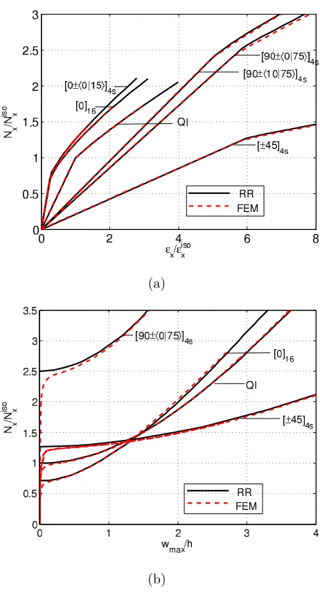
Fig. 2-a shows the normalised load vs normalised axial end-shortening strain curves for case A. For the constant stiffness laminates, the maximum compressive stiffness is, obviously, given by a [0]16 laminate, while [±45]4s
laminate has the maximum buckling load and very poor performance with respect to both the pre- and postbuckling stiffness. Three VAT laminates are selected for the comparison in Fig. 2-a. The [90± h0|75i]4s laminate has the
highest buckling load among all the VAT configurations [φ± hT0|T1i]4s with
linear variation of fibre angles (G¨urdal et al., 2008), however, its prebuckling and postbuckling axial stiffness is much lower than the quasi-isotropic and [0]16 laminates. On the other hand, the relative postbuckling stiffness of the
[90± h0|75i]4s VAT plate is relatively high (Kr = 0.56), which means there is
in the initial postbuckling regime. The VAT laminate [90±h10|75i]4sexhibits
higher value of relative postbuckling stiffness Kr = 0.71 compared to other
linear VAT configurations. VAT plate [0± h0|15i]4s exhibits the lowest
end-shortening strain, in other words the highest overall stiffness, under a given load (2Niso). Its prebuckling stiffness is almost the same as [0]16 but the
postbuckling stiffness is slightly improved. Fig. 2-b shows the normalised maximum transverse displacement wmax/h function vs the normalised axial
load. The maximum transverse deflection for [90± h0|75i]4s VAT laminate is
found to be much less than the other layups and this result demonstrates the considerable superiority of applying variable stiffness to restrict the maximum transverse deflection for a postbuckled laminated plate.
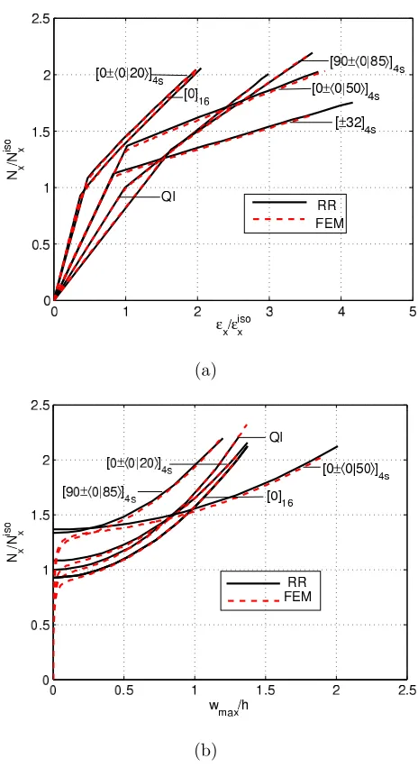
The postbuckling behaviour of plates under uniform compression with transverse edges constrained (case B) were studied and the results are shown in Fig. 3. The end-shortening curves in Fig. 3-a clearly show that both [±32]4s and [0± h0|50i]4s laminate exhibit high buckling load, but perform
poorly in the postbuckling regime. The fibre distribution of [0± h0|50i]4s
laminate gives rise to no re-distribution of the axial compression load, and provides much less contribution to improve postbuckling stiffness. The VAT plate [0±h0|20i]4sexhibits higher prebuckling and postbuckling stiffness than
the other [φ± hT0|T1i]4slayups (Fig.3-a) and the [0]16 laminate demonstrated
high overall stiffness value when compared to VAT laminates. Fig. 3-b shows the nonlinear transverse deflection response of different laminates and the VAT plate [90± h0|85i]4s demonstrates the lowest maximum transverse
displacement.
C are shown in Fig. 4, in which the results of case A are also presented (denoted by the dash-dot lines) for comparison purposes. For the boundary condition ofcase C, the prebuckling behaviour and the critical buckling state of the straight-fibre laminates and VAT plates with stiffness varying along y
direction (θ(y)) were observed to be identical tocase A(G¨urdal and Olmedo, 1993; G¨urdal et al., 2008). The postbuckling behaviour (stiffness) of straight-fibre laminates under case C are generally bounded in between the results of case A and case B (Bulson, 1970). The effects of in-plane boundary conditions on the postbuckling responses of VAT laminates largely depend on the distributions of their variable stiffness. Three VAT plates are shown in Fig. 4-a to illustrate the differences raised by the boundary conditions ofcase A andcase C on their postbuckling behaviour. The [0± h0|20i]4s plate gives
the highest overall stiffness among the VAT laminates with linear varation of fibre angles ([φ± hT0|T1i]4s) forcase C. Fig. 4-a shows that the postbuckling
stiffness of quasi-isotropic, 0◦ and VAT layup [0± h0|20i]4s under case C is
slightly higher than the result for case A. The differences in the load-end shortening behavior between case A and case C are much less for the other two VAT plates [90±h0|75i]4sand [90±h10|75i]4s. In particular, the solutions
of the [90± h0|75i]4s VAT laminate for case C are nearly the same as that of
case A. The load-transverse deflection curves for these laminates are plotted in Fig. 4-b, which demonstrates the similar trends with the results shown in Fig. 2-b for case A.
tow placement and deform in shear for towpreg techniques such as automatic fibre placement. As such, when a flat tow is curved, individual fibres slide to narrow the tow and minimise the excess length associated with outer radius compared with inner radius. In so doing, the tow thickens. Once all tows are laid down such thickness change manifests itself as a smooth variation across the plate (Kim et al., 2012). For example, the thickness along the transverse edges of the [90± h0|75i]4sVAT laminate or other analogous layups are likely
to be increased due to the maximum change in shifting angle. From the simu-lation results, it was observed that such a thickness build-up further improve the postbuckling stiffness (relative stiffness) of these VAT laminates. This suggests that the thickness variation offers us an additional design parameter to perform the postbuckling design of VAT laminates. However, a thorough study of the effects of thickness variation on the postbuckling behaviour of VAT laminate is beyond the scope of the paper and, it will be investigated in the future works.
5.2. Parametric study
A parametric study of postbuckling behaviour of square VAT plates with linear variation of fibre angles is presented in this section. The postbuckling analysis were carried out on the VAT laminates by varying the fibre angles
T0 and T1 (Eq. (1)) between 0◦ to 90◦ with a step of 5◦. Only the
varia-tion of fibre angles (stiffness) along y direction ([±θ(y)]4s) is considered in
this study, as these configurations demonstrate good buckling performance (G¨urdal et al., 2008; IJsselmuiden et al., 2010; Wu et al., 2012c) for the three in-plane boundary conditions. The relative stiffness Kr, postbuckling
of the VAT plates under the boundary conditions of case B and case C are computed. The results for case A are not presented, as it has been dis-cussed that this boundary case is similar to case C. The computed results
Kr, Kpost, Ko, Nxcr are normalised and shown in Figures 5 and 6 as functions
of the normalised prebuckling stiffness for case B and case C, respectively. Each curve in the figures represent a series of VAT plates with various values of T1 (from 0◦ at the left-end to 90◦ at the right-end), but with the same
value of T0, which is labeled in the figure. The red dash curve denotes the
result of straight-fibre laminates which vary from [90]16 to [0]16 as one moves
from left to right in each plot.
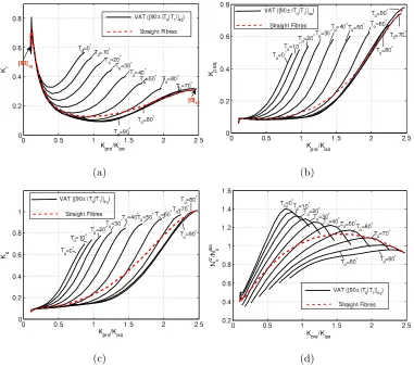
Forcase B, the largest relative stiffness shown in the Fig. 5-a isKr = 0.75
and is achieved by the VAT configuration [90± h0|25i]4s, which is slightly
more than the maximum valueKr = 0.73 given by the straight-fibre laminate
[±65]4s. But the prebuckling stiffness of these two laminates are relatively
low and results in poor behaviour of the overall stiffness. From Figs. 5-b and -c, the variation of postbuckling stiffness with respect to various VAT formats is very close to that describing the overall stiffness. The buckling performance of the VAT plates under case B is shown in Fig. 5-d. The [90± h0|80i]4s has the maximum normalised buckling load (Nxcr/Nxiso) 1.40,
which is 25% higher than the maximum value 1.12 obtained by a straight-fibre laminate [±30]4s. The [0]16 laminate exhibits the highest prebuckling
stiffness for the case of uniaxial compression and it also results in the largest postbuckling stiffness (overall stiffness) as shown in Figs. 5-b and -c. Nev-ertheless, if the VAT plate’s normalised prebuckling stiffness Kpre/Kiso is
significant and this phenomena is responsible for considerable improvement of the postbuckling responses. For prebuckling stiffness out of this range, the stress redistribution is primarily due to the von K´arm´an nonlinear strain-displacement relations governing the postbuckling behaviour. For instance, considering a VAT plate [90±h20|90i]4sand a straight-fibre laminate [±38]4s,
both of them approximately have an equivalent prebuckling stiffness as the quasi-isotropic laminate (Kpre = Kiso). The relative stiffness, postbuckling
stiffness, overall stiffness and buckling load of the VAT plate [90± h20|90i]4s
show an improvement of 291%, 317%, 230% and 15% over the straight-fibre laminate [±38]4s, respectively.
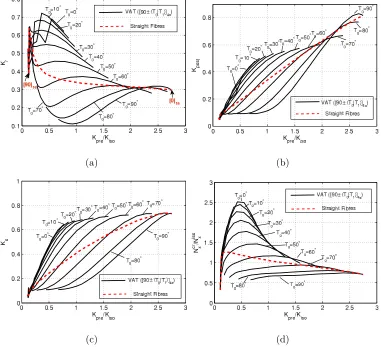
The superiority of VAT laminates with respect to the postbuckling re-sponses was also observed for case C, as shown in Fig. 6. The VAT plate [90± h10|70i]4s has the maximum relative stiffness Kr = 0.72 and exhibits
12% improvement over the maximum value 0.64 of a straight-fibre laminate [±55]4s. The sharp variation of postbuckling behaviour with small variations
postbuck-ling performance.
6. Conclusion
In this work, a semi-analytical variational approach was developed to perform postbuckling analysis of VAT plates under uniform axial compres-sion loading. The generality of the proposed approach was discussed and shown by modelling mixed stress/displacement boundary conditions. The different in-plane boundary conditions are implemented either using trigono-metric functions or Legendre polynomials. The postbuckling solutions for each boundary condition are determined using the proposed approach and validated with FEA to show the good accuracy, robustness and efficiency of this proposed approach.
vari-laminates were demonstrated.
Acknowledgments
The authors wish to acknowledge EPSRC, Airbus and GKN for support-ing this research under the project ABBSTRACT2 (EP/H025898/1).
Appendix
The explicit forms for the tensors in the postbuckling model (Eq. (22)) are expressed below. Each vectorized coefficient in Eq. (22) is reverted back to its matrix form, Wr orWs toWrs(W¯rs¯) and φp to φpq(φp¯q¯) (For example,
W0 =W00, W1 =W01, W2 =W02,· · · ,).
Kpimm(Kpqmmp¯¯q) =
Z 1
−1
Z 1
−1
µ4a11XpYq,ηηXp¯Yq,ηη¯ +
µ2a12(XpYq,ηηXp,ξξ¯ Yq¯+Xp,ξξYqXp¯Yq,ηη¯ )+
a22Xp,ξξYqXp,ξξ¯ Yq¯+µ2a66Xp,ξYq,ηXp,ξ¯ Yq,η¯ −
µ3a16(Xp,ξYq,ηXp¯Yq,ηη¯ +XpYq,ηηXp,ξ¯ Y¯q,η)− µa26(Xp,ξξYqXp,ξ¯ Yq,η¯ +Xp,ξYq,ηXp,ξξ¯ Yq¯)
dξdη
(29)
Klimc(Klmcp¯q¯) =
Z 1
−1
Z 1
−1
µ4a11ψlcXp¯Yq,ηη¯ +µ2a12ψlcXp,ξξ¯ Yq¯−
µ3a16ψlcXp,ξ¯ Yq,η¯
dξdη
(30)
Klimd(Klmdp¯q¯) =
Z 1
−1
Z 1
−1
µ2a12ψdlXp¯Yq,ηη¯ +a22ψldXp,ξξ¯ Yq¯−
µa26ψdlXp,ξY¯ q,η¯
dξdη
Krsimb(Krsmbr¯¯sp¯q¯) =1 2µ 2 Z 1 −1 Z 1 −1
Xr,ξYsX¯r,ξYs¯Xp¯Yq,ηη¯ +
XrYs,ηX¯rY¯s,ηXp,ξξ¯ Yq,ηη¯ +Xr,ξYsXr¯Ys,η¯ Xp,ξ¯ Yq,η¯
dξdη
(32)
Klicc(Klcc¯l) =
Z 1
−1
Z 1
−1
µ4a11ψlcψ c
¯
ldξdη (33)
Klicd(Klcd¯l ) =
Z 1
−1
Z 1
−1
µ2a12ψlcψ d
¯
ldξdη (34)
Krsicb(Krscb¯r¯s¯l) =
1 2µ 2 Z 1 −1 Z 1 −1
Xr,ξYsX¯r,ξYsψ¯ ¯lcdξdη (35)
Klidd(Kldd¯l ) =
Z 1
−1
Z 1
−1
a22ψdlψ d
¯
ldξdη (36)
Krsidb(Krsdbr¯s¯¯l) =
1 2µ 2 Z 1 −1 Z 1 −1
XrYs,ηXrY¯ s,ηψ¯ d¯ldξdη (37)
Kribb(Krsbbr¯s¯) =
Z 1
−1
Z 1
−1
D11Xr,ξξYsXr,ξξ¯ Y¯s
+µ2D12(XrYs,ηηXr,ξξ¯ Y¯s+Xr,ξξYsX¯rY¯s,ηη)
+µ4D22XrYs,ηηXr¯Ys,ηη¯ + 4µ2D66Xr,ξYs,ηXr,ξ¯ Y¯s,η
+ 2µD16(Xr,ξYs,ηXr¯Ys,ηη¯ +XrYs,ηηXr,ξ¯ Y¯s,ηη)
+ 2µ3D26(Xr,ξξYsX¯r,ξYs,η¯ +Xr,ξYs,ηXr,ξξY¯ ¯s)
dξdη
(38)
Krlibc(Krslbcr¯s¯) =µ2
Z 1
−1
Z 1
−1
Xr,ξYsψlcX¯r,ξYs¯dξdη (39)
Krlibd(Krslbdr¯¯s) = µ2
Z 1
−1
Z 1
−1
XrYs,ηψldX¯rY¯s,ηdξdη (40) Kpicm= (Klimc)T, Kpidm = (Klimd)T, Klidc = (Klicd)T (41)
References
Alhajahmad, A., Abdalla, M. M., G¨urdal, Z., 2010. Optimal design of tow-placed fuselage panels for maximum strength with buckling considerations. Journal of Aircraft 47 (3), 775 – 782.
Alhajahmad, A., Abdallah, M. M., G¨urdal, Z., 2008. Design tailoring for pres-sure pillowing using tow-placed steered fibers. Journal of Aircraft 45 (2), 630 – 640.
Bisagni, C., Vescovini, R., 2009a. Analytical formulation for local buck-ling and post-buckbuck-ling analysis of stiffened laminated panels. Thin-Walled Structures 47 (3), 318 – 334.
Bisagni, C., Vescovini, R., 2009b. Fast tool for buckling analysis and opti-mization of stiffened panels. Journal of Aircraft 46 (6), 2041 – 2053.
Budiansky, B., Hu, P. C., 1946. The lagrangian multiplier method of finding upper and lower limits to critical stresses of clamped plates. NACA, Report No. 848.
Bulson, P. S., 1970. The Stability of Flat Plates. Chatto and Windus Ltd, London.
Chia, C., Prabhakara, M., 1974. Postbuckling behavior of unsymmetri-cally layered anisotropic rectangular plates. Journal of Applied Mechanics, Transactions ASME 41 Ser E (1), 155 – 162.
Coan, J. M., 1950. Large deflection theory for plates with small initial cur-vature loaded in edge compression. Journal of Applied Mechanics 18, 143– 151.
Diaconu, C. G., Weaver, P. M., 2005. Approximate solution and optimum design of compression-loaded, postbuckled laminated composite plates. AIAA Journal 43 (4), 906 – 914.
Diaconu, C. G., Weaver, P. M., 2006. Postbuckling of long unsymmetrically laminated composite plates under axial compression. International Journal of Solids and Structures 43 (22-23), 6978–6997.
Feng, M., 1983. An energy theory for postbuckling of composite plates under combined loading. Computers and Structures 16 (14), 423 – 431.
G¨urdal, Z., Olmedo, R., 1993. In-plane response of laminates with spatially varying fiber orientations. variable stiffness concept. AIAA journal 31 (4), 751 – 758.
G¨urdal, Z., Tatting, B., Wu, C., 2008. Variable stiffness composite panels: Effects of stiffness variation on the in-plane and buckling response. Com-posites Part A: Applied Science and Manufacturing 39 (5), 911 – 922.
Harris, G., 1975. The buckling and post-buckling behaviour of composite plates under biaxial loading. International Journal of Mechanical Sciences 17 (3), 187 – 202.
pa-Jones, R. M., 1998. Mechanics of composite materials. CRC Press, 2nd Re-vised edition edition.
Kim, B. C., Potter, K., Weaver, P. M., 2012. Continuous tow shearing for manufacturing variable angle tow composites. Composites Part A: Applied Science and Manufacturing 43 (8), 1347 – 1356.
Levy, S., 1945. Bending of rectangular plates with large deflections. NACA, Report No. 737.
Mansfield, E. H., 1989. The bending and stretching of plates, Second Edition. Cambridge University Press.
Marguerre, K., 1937. The apparent width of the plate in compression. NACA, Report No. 833.
Pandey, M., Sherbourne, A., 1993. Postbuckling behaviour of optimized rect-angular composite laminates. Composite Structures 23 (1), 27 – 38.
Prabhakara, M. K., Chia, C. Y., 1973. Post-buckling behaviour of rectangular orthotropic plates. Journal of Mechanical Engineering Science 15 (1), 25– 33.
Rahman, T., Ijsselmuiden, S. T., Abdalla, M. M., Jansen, E. L., 2011. Postbuckling analysis of variable stiffness composite plates using a finite element-based perturbation method. International Journal of Structural Stability and Dynamics 11 (04), 735–753.
analysis of variable angle tow plates with general boundary conditions. Composite Structures 94 (9), 2961 – 2970.
Seresta, O., Abdalla, M. M., G¨urdal, Z., 2005. Optimal design of laminated composite plates for maximum post buckling strength. Collection of Tech-nical Papers - AIAA/ASME/ASCE/AHS/ASC Structures, Structural Dy-namics and Materials Conference 6, 4057 – 4068.
Sherbourne, A., Bedair, O., 1993. Plate-stiffener assemblies in uniform com-pression. part ii: Postbuckling. Journal of Engineering Mechanics 119 (10), 1956–1972.
Shin, D. K., Griffin, O. H., G¨urdal, Z., 1993. Postbuckling response of lam-inated plates under uniaxial compression. International Journal of Non-Linear Mechanics 28 (1), 95–115.
Stein, M., 1959. Loads and deformations of buckled rectangular plates. NASA Tech. Rep. R-40.
Wang, C.-T., 1952. Principle and application of complementary energy method for thin homogeneous and sandwich plates and shells with finite deflections. NACA, Report No. 2620.
Washizu, K., 1975. Variational Methods in Elasticity and Plasticity, Second Edition. Pergamon Press.
Wu, Z., Raju, G., Weaver, P. M., 2012b. Buckling analysis of vat plate using energy method. Collection of Technical Papers - 53rd AIAA/ASME Structures, Structural Dynamics and Materials Conference, 1–12.
Wu, Z., Weaver, P. M., Raju, G., Kim, B. C., 2012c. Buckling analysis and optimisation of variable angle tow composite plates. Thin-Walled Struc-tures 60 (0), 163 – 172.
Yamaki, N., 1959. Postbuckling behavior of rectangular plates with small initial curvature loaded in edge compression. Journal of Applied Mechanics 26, 407414.
A list of captions for the figures.
Figure 1: Boundary Conditions and Loading Cases.
Figure 2: Rayleigh-Ritz and FEA solutions of a square subjected to case A: (a) Normalised axial loads Nx/Nxiso versus Normalised axial strainx/isox
(b) Normalised axial loads Nx/Nxiso versus Normalized maximum transverse
displacement wmax/hfunction.
Figure 3: Rayleigh-Ritz and FEA solutions of a square subjected to case B: (a) Normalised axial loads Nx/Nxiso versus Normalised axial strain x/isox
(b) Normalised axial loads Nx/Nxiso versus Normalised maximum transverse
displacement wmax/hfunction.
Figure 4: Rayleigh-Ritz and FEA solutions of a square subjected to case C: (a) Normalised axial loads Nx/Nxiso versus Normalised axial strainx/isox
(b) Normalised axial loads Nx/Nxiso versus Normalised maximum transverse
displacement wmax/hfunction.
Figure 5: Postbuckling and buckling performance of square simply-supported laminates under uniform displacement compression and the transverse edges are constrained (case B). (a) Relative stiffnessKrversus Normalised
prebuck-ling stiffness (Kpre/Kiso) (b) Normalised postbuckling stiffness Kpost versus
Normalised prebuckling stiffness (c) Normalised overall stiffness Ko versus
Nor-malised prebuckling stiffness.
Figure 6: Postbuckling and buckling performance of square simply-supported laminates under uniform displacement compression and the transverse edges are free to move but keep straight (case C). (a) Relative stiffnessKr versus
Normalised prebuckling stiffness (Kpre/Kiso) (b) Normalised postbuckling
stiffness Kpost versus Normalised prebuckling stiffness (c) Normalised overall
stiffness Ko versus Normalised prebuckling stiffness (d) Normalised buckling
(a)
[image:39.612.190.421.144.572.2](b)
Figure 2: Rayleigh-Ritz and FEA solutions of a square simply-supported plate subjected
to case A: (a) Normalised axial loads Nx/Nxiso versus Normalised axial strain x/isox
(b) Normalised axial loadsNx/Nxisoversus Normalized maximum transverse displacement
(a)
[image:40.612.189.421.145.571.2](b)
Figure 3: Rayleigh-Ritz and FEA solutions of a square simply-supported plate subjected
to case B: (a) Normalised axial loads Nx/Nxiso versus Normalised axial strain x/isox
(b) Normalised axial loadsNx/Nxisoversus Normalised maximum transverse displacement
(a)
[image:41.612.191.421.154.562.2](b)
Figure 4: Rayleigh-Ritz and FEA solutions of a square simply-supported plate subjected
to case C: (a) Normalised axial loads Nx/Nxiso versus Normalised axial strain x/isox
(b) Normalised axial loadsNx/Nxisoversus Normalised maximum transverse displacement
(a) (b)
[image:42.612.116.497.173.511.2](c) (d)
Figure 5: Postbuckling and buckling performance of square simply-supported laminates
under uniform displacement compression and the transverse edges are constrained (case
B). (a) Relative stiffnessKrversus Normalised prebuckling stiffness (Kpre/Kiso) (b)
Nor-malised postbuckling stiffnessKpostversus Normalised prebuckling stiffness (c) Normalised
overall stiffness Ko versus Normalised prebuckling stiffness (d) Normalised buckling load
(a) (b)
[image:43.612.116.497.171.518.2](c) (d)
Figure 6: Postbuckling and buckling performance of square simply-supported laminates
under uniform displacement compression and the transverse edges are free to move but
keep straight (case C). (a) Relative stiffness Kr versus Normalised prebuckling stiffness
(Kpre/Kiso) (b) Normalised postbuckling stiffness Kpost versus Normalised prebuckling
stiffness (c) Normalised overall stiffness Ko versus Normalised prebuckling stiffness (d)