Visual pose estimation system for autonomous rendezvous of spacecraft

VISUAL POSE ESTIMATION SYSTEM FOR AUTONOMOUS RENDEZVOUS OF

SPACECRAFT

Mark A. Post1, Xiu T. Yan2, Junquan Li3, and Craig Clark4

1_{Lecturer, Space Mechatronic Systems Technology Laboratory. Department of Design, Manufacture and Engineering}

Management, University of Strathclyde, Glasgow, United Kingdom

2_{Professor, Space Mechatronic Systems Technology Laboratory. Department of Design, Manufacture and Engineering}

Management, University of Strathclyde, Glasgow, United Kingdom

3_{Marie Curie Experienced Researcher, Clyde Space Ltd. Glasgow, United Kingdom} 4_{CEO, Clyde Space Ltd. Glasgow, United Kingdom}

ABSTRACT

In this work, we consider a tracker spacecraft equipped with a short-range vision system that must visually iden-tify a target and determining its relative angular veloc-ity and relative linear velocveloc-ity using only visual informa-tion from an onboard camera. By means of visual feature detection and tracking across rapid, successive frames, features detected in two-dimensional images are matched and triangulated to provide three-dimensional feature maps using structure-from-motion techniques. Triangu-lated points are organized by means of orientation his-togram descriptors and used to identify and track targets over time. The state variables with respect to the camera system are extracted as a relative rotation quaternion and relative translation vector that are tracked by an embed-ded unscented Kalman filter. Inertial measurements over periods of time can then be used to determine the relative movement of tracker and target spacecraft. This method is tested using laboratory images of spacecraft movement with a simulated spacecraft movement model.

Key words: Satellite; Pose Estimation; Vision.

1. INTRODUCTION

Visual Pose Estimation technology has attracted a lot of interest for spacecraft navigation as an enabling tech-nology for rendezvous and docking manoeuvres. Guid-ance and Control of a spacecraft has been studied exten-sively, but in order for such systems to work effectively between spacecraft close to each other, the relative po-sition, attitude and and velocity between each spacecraft must be robustly estimated. The desired result is that two satellites will be able to reliably and autonomously ren-dezvous with each other, but visual position estimation for satellites in orbit is far from a solved problem.

Traditionally, RF radar trades off precision for wide range

of operation, and is not as suitable for uncooperative or small targets. The TriDAR system used a LIDAR and Iterative Closest Point system outside the ISS without approach or autonomy [RLB12]. Recent automated ren-dezvous and docking systems make use of optical, laser ranging, and LIDAR systems [HCDS14] [PHAR12] and visually-aided systems have been tested in proximity op-erations with NASA’s Space Shuttle, JAXA’s ETS-VII satellite [Oda00], and other satellites such as the DART mission [RT04].

However, the complexity, size, and power requirements of current LIDAR systems are still out of reach for small satellites and nanosatellites, and there is great potential in the use of multiple-view imaging and feature mapping since only one camera may be necessary. Many pose es-timation techniques have been proposed for this, and typ-ically focus on shape tracking and recognition, feature detection and triangulation [Sha14], or a combination of shape and features [TBB11]. The SPHERES experiment uses SURF feature matching with stereo vision for navi-gation inside the ISS [TSSO+14].

2. APPROACH AND TRACKING

To allow a tracker spacecraft to to identify and estimate the movement of a target spacecraft, we approach this problem as illustrated in Fig. 1 First, we build up a fea-ture set of points located in three dimensions by triangu-lation of keypoints on successive images of the target in the “Approach” phase. We then locate the camera rel-ative to the matched points by Perspective-n-Point (PnP) solution during the “Track” phase. By projecting the key-points into three dimensions, we build up a point cloud of the target over many more images in the “Observe” phase, which can then be matched in shape to a point cloud model, and the pose of the model accurately ob-tained by three-dimensional keypoint correspondences in the “Identify” phase.

Feature-based vision methods reduce complete images to a set of distinct, reproduceable “features” that are rep-resented by small numerical sequences. We apply ORB (Oriented FAST and Rotated BRIEF) point descriptors for 2-D feature matching with high rotation invariance [RRKB11]. We then use structure-from-motion methods to triangulate these points in space.

2.1. System Overview

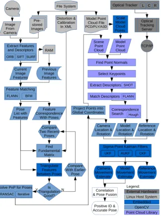
A flowchart of the process we propose is shown in Fig. 2, with details on each step provided in the following sec-tions. A sequence of images can be captured or cached, features extracted using two-dimensional point descrip-tors that are stored in memory and matched in pairs to obtain a list of images with features, and also a list of features tracked across images. This list of feature cor-respondences is used to track the movement of keypoints across several poses, and.if the triangulation is not good enough, a more different pose containing those features is selected. Using a pose solution, the points and cam-era are projected into global coordinates. The resulting scene point cloud can then be compared with a model cloud to identify the target by choosing a set of keypoints and extracting histogram descriptors for each with respect to point normals. By matching descriptors between the scene and model, the model and its pose can be found within the scene. An OptiTrak Trio optical tracking sys-tem is currently used as an external high-speed reference for pose estimation. The pose estimates are then filtered over time using an Unscented Kalman Filter to reduce noise. Sensor fusion of the triangulation and correspon-dence tracker-target measurements is planned, but has not been implemented yet.

2.2. Keypoint Detection and Matching

A method of keypoint detection must be used to obtain keypoints from a sequence of images. The FAST key-point detector (Features from Accelerated Segment Test) is frequently used for keypoint detection due to its speed,

and is used for quickly eliminating unsuitable matches in ORB. Starting with an image patchpof size31x31, each pixel is compared with a Bresenham circle built 45 de-grees at a time byx2

n+1 =x2n−2y(n)−1. The radius of the surrounding circle of points is nominally3, but is9

for the ORB descriptor, which expands the patch size and number of points in the descriptor. If at least75%of the pixels in the circle are contiguous and more than some threshold value above or below the pixel value, a feature is considered to be present [RD05]. The ORB algorithm introduces an orientation measure to FAST by computing corner orientation by intensity centroid, defined as

C=

m10 m00,

m01 m00

where mpq=X

x,y

xpyqI(x, y).

(1)

The patch orientation can then be found by θ =

atan2(m01, m10) and is Gaussian smoothed. ORB then applies the BRIEF feature descriptor fn(p) =

P

1≤i≤n2i−1τ(p;ai, bi), a bit string result of binary in-tensity testsτ, each of which is defined from the intensity p(a)of a point atarelative to the intensityp(b)at a point atbby [RD05]

τ(p;a, b) =

1 :p(a)< p(b) 0 :p(a)≥p(b)

(2)

The descriptor is also steered according to the orienta-tions computed for the FAST keypoints by rotating the feature set of points(ai, bi)in2xnmatrix form by the patch orientationθto obtain the rotated setF[RRKB11].

F =Rf

a1 · · · an b1 · · · bn

. (3)

The steered BRIEF operator used in ORB then becomes gn(p, θ) = fn(p) ∨ (ai, bi) ∈ F. A lookup table of steered BRIEF patterns is constructed from this to speed up computation of steered descriptors in subse-quent points.

Keypoints are then matched between two images in the sequence by attempting to find a corresponding keypoint a0 in the second image that matches each pointain the first image, which can be done exhaustively by anXOR operation between each descriptor and a population count to obtain the Hamming distance. However, The FLANN (Fast Library for Approximate Nearest Neighbor) search algorithm built into OpenCV is used in current work as it performs much faster while still providing good matches [ML09].

Figure 1. Process of Ego-Motion and Target Pose Estimation

coarsely pruned of bad pairings by finding the maxi-mum distance between pointsdmax and then removing all matches that have a coordinate distanceda of more than half the maximum distance between features using Mg=Mf(a)|da< dmax/2.

2.3. Three-Dimensional Projection

To obtain depth in a 3-D scene, an initial baseline for 3-D projection is first required using either stereoscopic vision, or two sequential images from different angles.. The Fundamental MatrixFis the transformation matrix that maps each point in a first image to a second image, and the set of “good” matches Mg is used where each keypointaiin the first image is expected to map to a cor-responding keypoint a0_i on the epipolar line in the sec-ond image by the relationa0T_i Fai = 0, i = 1, . . . , n [LF95]. For three-dimensional space, this equation is lin-ear and homogeneous and the matrixFhas nine unknown coefficients, so F can be uniquely solved for by us-ing eight keypoints with the method of Longuet-Higgins [LH87]. However, due to image noise and distortion, lin-ear least squares estimation (i.e. minFPi(a

0T

i Fai)2) or RANSAC [FB81] must be used to ensure that a “best” solution can be estimated. We use RANSAC for its speed to estimateFfor all matchesMgand estimate the associ-ated epipolar lines [FH03]while removing outliers more than0.1from their epipolar line fromMgto yield a final, reliable set of keypoint matchesMh. To perform a pro-jection into un-distorted space, a calibration matrixKis needed, either from calibration with a known pattern such as a checkerboard [Har97], or estimated for a sizew×h image as

K=

max(w, h) 0 w/2 0 max(w, h) h/2

0 0 1

!

. (4)

A camera matrix is defined asC =K[R|t]with the ro-tation matrixRand the translation vectortdefining the pose of the camera in space, and for two images, we de-fine two camera matricesC1andC2. To localize a point in un-distorted space, we formulate the so-called essen-tial matrixE=t×R=KT_{FKthat relates two} match-ing undistorted points xˆ andxˆ0 in the camera plane as

ˆ

a0T_i Eˆai = 0, i = 1, . . . , n[HS97]. In this way,E in-cludes the “essential” assumption of calibrated cameras [Shi12b], and is related to the fundamental matrix byE

After calculatingE, we can find the location of a second cameraC2by assuming for simplicity that the first cam-era is uncalibrated and located at the origin (C1= [I|0]). We decomposeE =t×Rinto its componentRandt

matrices by using the singular value decomposition ofE

[HZ04]. We start with the orthogonal matrixWand and singular value decomposition (SVD) ofE, defined as

W=

0 −1 0

1 0 0

0 0 1

!

SVD(E) =U

1 0 0

0 1 0

0 0 0

!

V.

(5)

The matrixWdoes not directly depend on E, but pro-vides a means of factorization for E. Detailed proofs can be found in [HZ04] and are not reproduced here, but there are two possible factorizations of R, namely

R = UWT_VT _{and R = UWV}T_{, and two} possi-ble choices for t, namely t = U(0,0,1)T _{and t =}

−U(0,0,1)T. Thus when determining the second cam-era matrixC2=K[R|t], we have four choices in total.

it is now possible to triangulate the original un-distorted point positions in space with E and a pair of matched keypoints[a= (ax, ay),b= (bx, by)]∈Mhusing itera-tive linear least-squares triangulation [HS97]. A point in three dimensionsx = (xx, xy, xz,1)written in the ma-trix equation formAx = 0results in four linear nonho-mogeneous equations in four unknowns for an appropri-ate choice ofA4x4. To solve this, we can write the system asAx=B, withx= (xx, xy, xz), andA4x3andB4x1 as defined by Shil [Shi12a]. The solutionxby SVD is transformed to un-distorted space by ˆx = KC1x, as-suming that the point is neither at0nor at infinity. This triangulation must be performed four times for each com-bination ofRandtand tested by perspective transforma-tion withC1andxˆz>0to ensure the resulting pointspi are in front of the camera.

2.4. Image Selection

Using adjacent pairs of images in a closely-spaced time sequence allows feature points to be tracked more reli-ably between images, as there is less chance of condi-tions or change in angle causing a feature to change sig-nificantly. However, the disadvantage of using closely-spaced images for pose estimation is that a very small angular difference between two images will prevent trian-gulation solutions, like very distant points. Therefore, we track, match, and store keypoints between closely-spaced images, but only triangulate with images that are well-separated that contain tracked keypoints between the two. Unusable images in the matching process are most com-monly due to:

• Not enough feature points being matched to obtain

For triangulate

• Inaccurate estimates of rotationRand translationt

• Inaccuracy of the fundamental matrixF, preventing decomposition toE,R, andt

until a predefined “reset” limit. Valid matches from the new imagePtor later are added the the existing tracked keypoint list to associate feature numbers across the se-quence of images. When obtaining the fundamental ma-trixF, only keypoints that have been associated between both images are used.

2.5. Position Estimation

To finding the ego-motion of the tracker’s camera relative to feature points represents the Perspective & Point (PnP) problem. For this, we apply the OpenCV implementation of the EPnP algorithm [MNLF07]. For then-point cloud with points p1. . .pn, four control points ci define the world coordinate system and are chosen with one point at the centroid of the point cloud and the rest oriented to form a basis. Each reference point is described in world coordinates (denoted withw) as a linear combination of ci with weightingsαij. This coordinate system is con-sistent across linear transforms, so they have the same combination in the camera coordinate system (denoted withc_{. The known two-dimensional projectionsu}

iof the reference pointspiare linked to these weightings byK considering that the projection involves scalar projective parameterswi, leading to the following.

pw_i =

4

X

j=1

αijcw_j, pc_i =

4

X

j=1 αijcc_j,

4

X

j=1

αij= 1 (6)

Kpc_i =wi

ui 1 =K 4 X j=1

αijccj (7)

The expansion of this equation has12unknown control points and n projective parameters. Two linear equa-tions can be obtained for each reference point to ob-tain a system of the form Mx = 0, where the null space or kernel of the matrix M2nx12 gives the solu-tion x = [cc₁T,cc₂T,cc₃T,cc₄T] to the system of equa-tions, which can be expressed asx = Pm

i=1βivi. The setvi is composed of the null eigenvectors of the prod-uctMT_{Mcorresponding tomnull singular values ofM.} The method of solving for the coefficientsβ1. . . βm de-pends on the size ofm, and four different methods are used in the literature [MNLF07] for practical solution.

Let the translation and rotation in world coordinates of the previous pose be tw(t −1) and Rw(t − 1), and that of the current pose be tw(t) and Rw(t), for which we need to find the current camera matrix in world coordinates Cw(t). The relative transformation between the camera positions t(t) and R(t) is used to incrementally advance the current pose (assumed to be attached rigidly to the camera) as Cw(t) =

[Rw(t−1)R(t)|R(t) (t(t) +tw(t−1))]., and feature points are incrementally projected into world coordi-nates with x0 = (Rw(t−1)R(t))

T

x + Rw(t −

1) (t(t) +tw(t−1)). Orientation is stored as a quater-nion from the elementsrij ofRw.

q=    w x y z   =      √

1+r00+r11+r22

2 r21−r12

2√1+r00+r11+r22

r02−r20

2√1+r00+r11+r22

r10−r01

2√1+r00+r11+r22

     (8)

3. OBSERVATION AND IDENTIFICATION

The PnP solution across a sequence of images allows us to track the pose of the tracker spacecraft relative to fea-tures on the target spacecraft. However, in most cases it is necessary to identify what the actual orientation of the target is with respect to a known geometric model, or to identify specific parts of the target for interaction or analysis. For this task, we use the positional corre-spondences of three-dimensional keypoints selected from the constructed point cloud with respect to keypoints se-lected from a reference model point cloud that can be ob-tained in advance or on-line from another sequence of images with known relative pose. Model recognition is done on a per-pose basis with accumulated points in the point cloud once a sufficient number of images has been acquired during the “Observation” phase. This makes it possible to match parts of a structure without requiring the entire structure to have keypoints, for example if the target is in partial shadow. We use an Unscented Kalman filter (UKF) for reducing noise over time for pose mates. Separate filtering is performed for the pose mates obtained from PnP solutions and target pose esti-mation, both translation and quaternion rotation, using a fast embedded UKF implementation with adaptive statis-tics [LPL13].

3.1. Object Pose Estimation

A set of three-dimensional keypoints are chosen from both the scene and the model by picking individual points from the cloud separated by a given sampling radius. Normals are calculated for these keypoints relative to nearby points so that each keypoint has a repeatable ori-entation. The keypoints are then associated with three-dimensional SHOT (Signature of Histograms of Orien-Tations) descriptors [STDS14]. SHOT descriptors are calculated by grouping together a set of local histograms over the volumes about the keypoint, where this volume is divided into by angle into 32 spherically-oriented spa-tial bins. Within a given radius of the keypoint, point counts from the local histograms are binned as a cosine functioncos(θi) =nu·nvi of the angleθibetween the

point normal within the corresponding part of the struc-turenvi and the feature point normal nu. This has the

differ-ences in relative directions, and creating a coarse parti-tioning that can be calculated fast with small cardinality.

Comparing the scene keypoint descriptors with the model keypoint descriptors to find good correspon-dence matches is done using a FLANN search on a k-dimensional tree (k-d tree) structure, similarly to the matching of image keypoints. Additionally, the BOrder Aware Repeatable Directions algorithm for local refer-ence frame estimation (BOARD) is used to calculate local reference frames for each three-dimensional SHOT de-scriptor [PDS11] to make them independent of global co-ordinates for rotation and translation invariance. Once a set of nearest correspondences and local reference frames is found, clustering of correspondences to given clus-ter sizes is performed by pre-computed Hough voting to make recognition of shapes more robust to partial occlu-sion and clutter [TDS10].

Evidence of a particular pose and instance of the model in the scene is initialized before voting by obtaining the vector between a unique reference point CM _{and each} model feature point FM

i and transforming it into lo-cal coordinates by the transformation matrix RM

GL =

[LM

i,x, LMi,y, LMi,z]T from the local x-y-z reference frame unit vectors LM

i,x, LMi,y, and LMi,z. This precomputation can be done offline for the model in advance and is per-formed by calculating for each feature a vectorVM

i,L =

[LM

i,x, LMi,y, LMi,z]·(CM −FiM). For online pose estima-tion, Hough voting is performed by each scene feature FS

j that has been found by FLANN matching to corre-spond with a model featureFM

i , casting a vote for the po-sition of the reference pointCM _{in the scene. The} trans-formationRM_S

Lthat makes these points line up can then be transformed into global coordinates with the scene ref-erence frame unit vectors, scene refref-erence pointFS

j and scene feature vector VS

i,L as Vi,GS = [Lj,xS , LSj,y, LSj,z]· VS

i,L+F S

j . The votes cast byVi,GS are thresholded to find the most likely instance of the model in the scene, al-though multiple peaks in the Hough space are fairly com-mon and can indicate multiple possibilities for model in-stances. Due to the statistical nature of Hough voting, it is possible to recognize partially-occluded or noisy model instances, though accuracy may be lower.

3.2. Processing Times

To profile the processing requirements of the described algorithms on a system that could potentially be embed-ded into a satellite, the algorithm was run on a667M Hz ARM Cortex-A9 processor with pre-defined images of a CubeSat engineering model in VGA resolution and pre-computed point clouds, and raw timing statistics gathered for the processing time of each algorithm. Tests 1 and 2 were performed with6524model points and5584scene points from220images, and tests3and4were performed with6524model points and 1816scene points from32

images. Tests 1 and 3 were performed with a descriptor radius of0.05and cluster size of0.1, and Tests 2 and 4

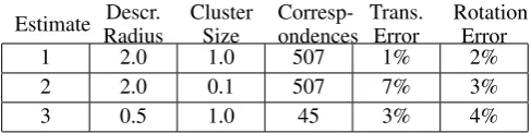
Table 3. Correspondences and Error resulting from vary-ing Descriptor Radius and Cluster Size

Estimate Descr. Radius

Cluster Size

Corresp-ondences

Trans. Error

Rotation Error

1 2.0 1.0 507 1% 2%

2 2.0 0.1 507 7% 3%

3 0.5 1.0 45 3% 4%

were performed with a descriptor radius of0.1and cluster size of0.5. Tab. 1 and Tab. 2 show the timing informa-tion obtained for each of the described algorithms in these cases.

3.3. Identification Accuracy

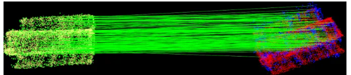
To illustrate the accuracy of pose estimation while vary-ing the descriptor radius and cluster size and therefore processing times, a set of pose estimation tests were per-formed using a CubeSat engineering model as a target for pose identification. In three examples of target identifica-tion shown in Fig. 3, Fig. 4, and Fig. 5, high-density model points are in yellow with selected keypoints in green, and low-density scene keypoints are shown in blue. The model instance found in the scene is over-laid in red from a high-density model composed of26339

points, while the scene is composed of1960points trian-gulated from52images. The number of keypoints was reduced by radius to2042in the model and1753in the scene. The descriptor radius and cluster size for these estimates, with the resulting number of correspondences and rounded cumulative errors in translation and rotation are shown in Tab. 3.

As more scene points are added over time, accuracy can increase, but only if they are consistent with the exist-ing scene. We can see from these results that increasexist-ing the size of the SHOT descriptor will increase the number of keypoints available and result in better accuracy and higher likelihood of identifying a shape, but also will re-quire longer processing times. Cluster sizes must be set appropriately for the point cloud size, as a cluster size too small or too large will prevent valid instances from being found, and result in decreased accuracy.

4. CONCLUSIONS

Table 1. Timing for Features, Triangulation and PnP

Test Number

Feature Detect.

Feature Matching

Feature Selection

Fundam. Matrix

Essential Matrix

Triangu-lation

PnP RANSAC

Ego-Motion

Total Time 1-2 0.12 0.058 0.015 0.083 0.0017 0.038 0.0033 0.0005 0.32 3-4 0.12 0.061 0.010 0.048 0.0014 0.025 0.0026 0.0004 0.27

Table 2. Timing for Correspondence and Identification

Test Number

Model Normals

Scene Normals

Model Sampling

Scene Sampling

Model Keypoints

Scene Keypoints

FLANN Search

Cluster-ing

Total Time 1 0.17 0.15 0.027 0.020 1.26 0.84 107.7 0.92 112.1 2 0.17 0.15 0.029 0.024 3.37 2.19 118.0 2.00 127.2 3 0.17 0.043 0.031 0.0083 3.31 0.37 42.5 0.63 48.4 4 0.17 0.041 0.031 0.0078 3.31 0.37 42.6 1.36 49.1

Figure 3. Pose Correspondence for Estimate 1, Descriptor Radius2.0, Cluster Size1.0

Figure 4. Pose Correspondence for Estimate 1, Descriptor Radius2.0, Cluster Size0.1

ORB algorithm that combines FAST keypoint detection and BRIEF feature descriptors provides good tolerance to rotation and scaling of features for this purpose. For useful reconstruction, it is important to identify as many features as possible, so target spacecraft with many col-ors, edges, and shapes generally provide the best results for feature-based systems such as this. It is important to note that this method of motion estimation provides best solutions through post-processing of results. The more images that are included when creating the structure, the better triangulation will be. If processing power and stor-age is available to include a large number of recent im-ages, such as by observing the target through multiple rotations, a better solution for motion will be obtained. To additionally decrease the processing time if desired, the camera image can be lowered in resolution, or pixels can be under-sampled by choosing only every 2nd pixel or every 4th pixel in a staggered pattern over the image for feature matching [AZK09].

It is intended that even small spacecraft such as nanosatellites with a single camera could take advantage of this system. Work is underway to scale this system to a level suitable for nanosatellite use, which could provide a technology demonstration with a minimum of cost and risk. As the performance of feature tracking depends very heavily on the design of the feature descriptor and method of matching, further comparison of descriptor types for both two-dimensional and three-dimensional matching is warranted. Future work also includes the validation of these methods on a variety of models, and under a broader set of varying conditions to evaluate the robustness of feature-based systems. A wide variety of applications for this technology is also available, including robotic uses and planetary rover navigation and sensing.

REFERENCES

[AZK09] K. Ambrosch, C. Zinner, and W. Kubinger. Algorithmic considerations for real-time stereo vision applications. In

MVA09, page 231, 2009.

[FB81] Martin A. Fischler and Robert C. Bolles. Random sample consensus: a paradigm for model fitting with applications to image analysis and automated cartography. Commun. ACM, 24(6):381–395, June 1981.

[FH03] C. L. Feng and Y. S. Hung. A robust method for estimating the fundamental matrix. InIn International Conference on Digital Image Computing, pages 633–642, 2003. [Har97] Richard Hartley. Self-calibration of stationary cameras.

In-ternational Journal of Computer Vision, 22(1):5–23, 1997. [HCDS14] Heather Hinkel, Scott Cryan, Christopher DSouza, and Matthew Strube. Nasa’s automated rendezvous and dock-ing/capture sensor development and its applicability to the ger. 2014.

[HS97] Richard I. Hartley and Peter Sturm. Triangulation. Com-puter Vision and Image Understanding, 68(2):146 – 157, 1997.

[HZ04] R. I. Hartley and A. Zisserman. Multiple View Geometry in Computer Vision. Cambridge University Press, ISBN: 0521540518, second edition, 2004.

[LF95] Q.-T. Luong and O.D. Faugeras. The fundamental matrix: theory, algorithms, and stability analysis. International Journal of Computer Vision, 17:43–75, 1995.

[LH87] H. C. Longuet-Higgins. A computer algorithm for recon-structing a scene from two projections. In Martin A. Fis-chler and Oscar Firschein, editors,Readings in computer vision: issues, problems, principles, and paradigms, pages 61–62. Morgan Kaufmann Publishers Inc., San Francisco, CA, USA, 1987.

[LPL13] J. Li, M. A. Post, and R. Lee. A novel adaptive unscented kalman filter attitude estimation and control system for a 3u nanosatellite. In12th biannual European Control Confer-ence, Zurich, Switzerland, 17-19 July 2013.

[ML09] Marius Muja and David G. Lowe. Fast approximate nearest neighbors with automatic algorithm configuration. In Inter-national Conference on Computer Vision Theory and Ap-plication (VISSAPP’09), pages 331–340. INSTICC Press, 2009.

[MNLF07] F. Moreno-Noguer, V. Lepetit, and P. Fua. Accurate non-iterative o(n) solution to the pnp problem. InIEEE Inter-national Conference on Computer Vision, Rio de Janeiro, Brazil, October 2007.

[Oda00] Mitsushige Oda. Experiences and lessons learned from the ets-vii robot satellite. InRobotics and Automation, 2000. Proceedings. ICRA’00. IEEE International Conference on, volume 1, pages 914–919. IEEE, 2000.

[PDS11] Alioscia Petrelli and Luigi Di Stefano. On the repeatability of the local reference frame for partial shape matching. In

Computer Vision (ICCV), 2011 IEEE International Confer-ence on, pages 2244–2251. IEEE, 2011.

[PHAR12] Jose Padial, Marcus Hammond, Sean Augenstein, and Stephen M Rock. Tumbling target reconstruction and pose estimation through fusion of monocular vision and sparse-pattern range data. InMultisensor Fusion and Integration for Intelligent Systems (MFI), 2012 IEEE Conference on, pages 419–425. IEEE, 2012.

[RD05] Edward Rosten and Tom Drummond. Fusing points and lines for high performance tracking. InComputer Vision, 2005. ICCV 2005. Tenth IEEE International Conference on, volume 2, pages 1508–1515 Vol. 2, 2005.

[RLB12] St´ephane Ruel, Tim Luu, and Andrew Berube. Space shut-tle testing of the tridar 3d rendezvous and docking sensor.

Journal of Field Robotics, 29(4):535–553, 2012.

[RRKB11] Ethan Rublee, Vincent Rabaud, Kurt Konolige, and Gary R. Bradski. Orb: An efficient alternative to sift or surf. InICCV 2011, pages 2564–2571, 2011.

[RT04] Michael Ruth and Chisholm Tracy. Video-guidance design for the dart rendezvous mission. InDefense and Security, pages 92–106. International Society for Optics and Photon-ics, 2004.

[Sha14] S. Sharma. Pose estimation of uncooperative spacecraft us-ing monocular vision. InInvited Student Presentation at Stanford’s 2014 PNT Challenges and Opportunities Sym-posium, Kavli Auditorium, SLAC, 10 2014.

[Shi12a] Roy Shil. Simple triangulation with opencv from harley & zisserman. Online, January 2012.

[Shi12b] Roy Shil. Structure from motion and 3d reconstruction on the easy in opencv 2.3+. Online, February 2012. [STDS14] Samuele Salti, Federico Tombari, and Luigi Di Stefano.

Shot: unique signatures of histograms for surface and tex-ture description.Computer Vision and Image Understand-ing, 125:251–264, 2014.

[TDS10] Federico Tombari and Luigi Di Stefano. Object recognition in 3d scenes with occlusions and clutter by hough voting. In

Image and Video Technology (PSIVT), 2010 Fourth Pacific-Rim Symposium on, pages 349–355. IEEE, 2010. [TSSO+_{14] Brent E Tweddle, Timothy P Setterfield, Alvar}