A Topological Model For A 3-Dimensional
Spatial Information System
by
Simon Pigat, B.Surv. (Hons.)
A thesis submitted in fulfilment of the requirements for the degree of
Doctor of Philosophy University of Tasmania
Statement
Except as stated herein, this thesis contains no material which has been accepted for the award of any .other degree or dipl6ma.in any university, and to the best of my
knowledge and belief, it contains no copy or paraphrase of material previously published or written by another person, except where due reference is made.
Simon Phillip Pigot
Dept of Surveying and Spatial Information Science & Dept. of Computer Science,
University of Tasmania September, 1995
This thesis may be made available for loan and limited copying in accordance with the Copyright Act 1968.
Abstract
This thesis proposes the topological theory necessary to extend the conventional topological models used in geographic information systems (GIS), computer-aided design (CAD) and computational geometry, to a 3-dirnensional spatial information system (SIS) which supports query and analysis of spatial relationships.
To encompass a wide range of applications and minirniz.e fragmentation, we define a spatial object as a cell complex, where each k-cell is homeomorphic to a Euclidean k-manifold with one or more subdivided (k-1)-k-manifold boundary cycles. The sirnplicial and regular cell complexes currently used in topology and many spatial information systems, are restricted forms of these generaliz.ed regular cell complexes.
Spatial relationships between the cells of the generalized regular cell complex are expressed
4i
terms of their boundary and coboundary cells. To support query and traversal of the neighborhood of any cell via orderings of its cobounding cells, we embed the generalized regular k-cell complex in a Euclidean n-manifold which we represent as a 'world' n-cell.Spatial relationships between spatial objects can be expressed in terms of the boundary and co boundary relations between the cells of another complex formed from the union of the generalized regular cell complexes. If this complex is embedded in a Euclidean n-manifold, then co bounding cells may also be ordered. The cells of this complex have 'singular manifold' or 'pseudomanifold' boundary cycles, which we classify into three primitive types using identification spaces. The cell complex is known as the generaliz.ed singular cell complex - generalized regular, regular and simplicial complexes are
restricted forms of this complex.
Topological operators are defined to construct spatial objects. Since the set of spatial objects has few restrictions, we define topological operators which consistently construct both subdivided manifolds and manifolds with boundary, from the strong deformation retract of a manifold with boundary. The theory underlying these operators is based on combinatorial homotopy. Generic versions of these topological construction operators can then be used to join these subdivided manifolds or manifolds with
boundary, to form the generalized regular cell complex.
Acknowledgements
I would like to express my gratitude to my supervisors, Associate Professor Peter Zwart and Dr. Chris Keen for their support and encouragement throughout this research. Many other people have contributed to this thesis both directly and indirectly. Specifically, I would like to thank Geoff Whittle and Jeff Weeks for help and
encouragement with the theory of topology; Erik Brisson, Jim Farquhar, Wm. Randolph Franklin, Mark Ganter, Bill Hazelton, Scott Morehouse, George Nagy, Alan Saalfeld, Kevin Weiler, Tom Wood and the anonymous referees of the published papers, for reviews, directions, encouragement and discussions (no matter how short or extended!) on various aspects of this research.
I would particularly like to thank those topologists who do not believe that demonstrating their intuition causes confusion: G. Francis for A Topological
Picturebook -Francis (1987), K. Janich for Topology - Janich (1980), J. Scott Carter for How Surfaces Intersect in Space: An Introduction to Topology -Scott Carter (1993), J. Stillwell for Classical Topology and Corhhinatorial Group Theory -Stillwell (1980) and J. Weeks for The Shape of Space: How to Visualize Surfaces and Three-Dimensional Manifolds-Weeks (1990). Also, I would like to thank James P. Corbett and Marvin S. White for their seminal works on the application of topology to
geographic and spatial information systems.
I acknowledge the receipt of a Commonwealth Postgraduate Scholarship for the years 1988-90 and 1991-92 inclusive.
Table of Contents
Abstract ...
iAcknowledgements ...
iiiTable of Contents ...
ivList of Figures ...
viiiChapter 1 - Introduction ... 1
1.1 Introduction ... 1
1.2 A Spatial Information System for 3-Dimensional Applications ... .4
1.3 Topology ... 5
1.4 Spatial Objects and Cell Complexes ... 5
1.4.1 Relationships between the cells in the cell complex ... 7
1.4.2 Relationships between distinct cell complexes ... 12
1.4.3 Representing the Cell Complexes ... 14
1.5 Topological Operators ... 14
1.6 Overview of this Thesis ... 17
Chapter 2 - Review of Existing Topological Models ...
~...
192.1 Introduction and Taxonomy of Topological Models ... 19
2.2 Map Models Used in 2-Dimensional GIS ... 21
2.3 Subdivisions of 2-manifolds ... 25
2.3.1 Winged-Edge ... 25
2.3.2 Quad-Edge ... 26
2.3.3 Half-Edge ... 27
2.4 Subdivisions of 3-Manifolds ... 29
2.4.1 Face-Edge ... 29
2.4.2 Facet-Edge ... 30
2.5 Subdivisions of n-manifolds and n-manifolds with boundary ... .31
2.5.1 Cell-Tuple ... 31
2.5.2 Winged-Representation ... 34
2.6 Other Subdivisions ... 36
2.6.1 Corbett's General Topological Model For Spatial Reference ... .36
2.6.2 Non-Manifold Subdivisions - The Radial Edge ... 38
2.6.3 N-Dimensional Generalized Maps ... .40
2.6.4 Selective Geometric Complexes ... 44
2.6.5 Tri-Cyclic Cusp ... 48
Chapter 3 - Mathematical Background ...
573.1 Introduction ... 57
3.2 The Continuous Maps - Homeomorphism and Homotopy ... 58
3.3 Manifolds and Manifolds with Boundary ... 61
3.3.1 Homeomorphism Types ... 63
A. Manifolds ... 63
B. Manifolds With Boundary ... 63
3.3.2 Homotopy Type ... 66
A.
Manifolds With Boundary ... : ... 66B. Manifolds ... 68
3.3.3 Table of Homeomorphism and Homotopy Types ... 68
Chapter 4 - Generalized Regular Cell Complexes ...
694.1 Introduction ... 69
4.2 Simplicial, Regular and CW Complexes ... 70
4.3 Generalized Regular Cell Complexes ... 77
4.4 Fundamental group (1-dimensional homotopy group) ... 80
4.5 Homology groups ... 86
4.6 Ordering and Representation of Cell Neighborhoods ... 87
4.6.1 0-dimensional Spatial Object in RD (1SnS3) ... 93
4.6.2 1-dimensional Spatial Object in RD (1SnS3) ... 94
4.6.3 2-dimensional Spatial Object in RD (2 Sn S 3) ... 96
4.6.4 3-dimensional Spatial Object in R3 ... 99
4.6.5 Summary ... 100
4.6.6 Discussion ... 103
Chapter 5 - Generalized Singular Cell Complexes ... 106
5.1 Introduction ... 106
5.2 Modelling Spatial Relationships between Spatial Objects ...
108
. 5.2.1 Object Based ... 110
5.2.2 Cell Complex ... 111
5.3 Generalized Singular Cell Complexes ... 113
5.4 Classification of Pseudomanifold Boundary Cycles ... 114
5.4.1 Type 1 Pseudomanifolds ... 119
A. n-point ... 120
B. n-line/n-line with pinchpoint ... 121
5.4.2 Type 2 Pseudomanifolds ... 122
5.4.3 Type 3 Pseudomanifolds ... 122
5.4.4 Summary ... 123
5.5 Analysis of Ordering Results ... 125
5.5.1 Internal Cell Complexes ... 125
A. Internal to a Generalized Singular 2-Cell ... 126
B. Internal to a Generalized Singular 3-Cell ... 127
5.5.2 Analysis of Circular Orderings ... 127
A. Generalized Singular 2-Cells ... 127
B. Generalized Singular 3-Cells ... 129
5.5.3 Analysis of Subspace Orderings ... 132
5.5.4 Summary ... 134
Chapter 6 - Topological Operators ... 144
6.1 Introduction ... 144
6.2 Review of Existing Topological Operators ... 146
6.2.1 The Euler Operators for Subdivisions of 2-Manifolds ... 146
6.2.2 Generic Cell Complex Construction Operators ... 150
6.2.3 Extending the Generic Cell Complex Construction Operators ... 154
A. Generalized Regular Cells with more than one Boundary Cycle ... ~ ... 156
B. Elift: ... .;;. ...
156-C. Ejoin ... 158
6.2.4 Overview of the Combinatorial Homotopy Operators ... 163
6.3 Development of the Combinatorial Homotopy Operators ... 165
6.3.1 Homotopy Equivalence- and the Strong Deformation Retract ... 165
6.3.2 Combinatorial Homotopy ... 169
A. Constructing a Subdivided 2-Manifold with Boundary ... 177
B. Constructing a Subdivided 2-Manifold ... 178
6.4 Building the Topology of a Subdivided Manifold/Manifold with Boundary from a 1-Skeleton ... 181
6.4.1 Review of Existing Topology Reconstruction Algorithms ... 181
A. Planar Sweep ... 181
B. Wire Frame Reconstruction Algorithms ... 183
6.4.2 The Extended Topology Reconstruction Algorithm ... 191
A. Overview ... 200
B. Implementation ... 202
C. Example ... 203
D. Assembling the Subdivided Manifold/Manifold With Boundary ... 210
Chapter 7 - Conclusions ... 211
7 .1 Synopsis ... 211
7 .2 Future Research ... 212
7.2.1 Arcs ... 213
7 .2.2 Implementation ... : ... 213
7.2.3 Higher-Dimensional Applications ... 214
7.2.4 Topological Operators ... 215
References ... 219
Publications
1. Pigot, S., 1991, Topological Models for 3D Spatial Information Systems, Proceedings of AutoCarto-10, Baltimore, Maryland, USA pp. 368-392
2. Pigat, S., 1992, A Topological Model for a 3D Spatial Information System, Proceedings of the 5th International Symposium on Spatial Data Handling (ed. D. Cowen), Charleston, South Carolina, USA, vol. 1, pp. 344-360
3. Pigat, S. & B. Hazelton, 1992, The Fundamentals of a Topological Model for a Four-Dimensional GIS, Proceedings of the 5th International Symposium on Spatial Data Handling (ed. D. Cowen), Charleston, South Carolina, USA, voL 2, pp. 580-591
4. Pigat, S., 1994, Generalized Singular 3-Cell Complexes, Proceedings of the 6th International Symposium on Spatial Data Handling (ed.
T.C.
Waugh &List of Fi.gures
Figure 1.1 - 2-manifold and 2-manifold with boundary ... 6
Figure 1.2 - 3-cell as a Euclidean 3-manifold with 2-manifold boundary ... 7
Figure 1.3 - some complex spatial objects for 3-dimensional applications ... 8
Figure 1.4 - coboundary orderings in a subdivided 2-manifold ... 9
Figure 1.5 ~ coboundary orderings in a subdivided 3-manifold ... 10
Figure 1.6 - coboundary orderings in a subdivided I-manifold ... 11
Figure 1.7 - singular 2-cells ... 13
Figure 2.1 - a singular 2-cell ... ... : ... 22
Figure 2.2 - formation of a singular cell ... 22
Figure 2.3 - cyclic singularities generated by identifying points ... 23
Figure 2.4 - a singular cell complex and its dual construction ... 24
Figure 2.5 - the winged-edge template ... 25
Figure 2.6 - the four directed oriented edges associated with an edge ... 26
Figure 2.7 - the face-edge template ... 30
Figure 2.8 - cell-tuples in a fragment of a subdivided 2-manifold ... 32
Figure 2.9 - the graph formed by cell-tuples and switch operations ... : ... 33
Figure 2.10- combinatorial map of Vince (1983) ... 41
Figure 2.11 - examples of n-G-maps ... 43
Figure 2.12 - a simple SGC consisting of a face with planar extent and an edge with linear extent ... 46
Figure 2.13 - an example of a simple 2-dimensional SGC ... 47
Figure 2.14 - cusps and cycles of cusps ... 50
Figure 2.15 - the loop cycles of cusps of a wall ... 51
Figure 2.16 - the disk cycle of cusps ... 51
Figure 2.17 - edge orientation cycle ... 52
Figure 2.18 - the alternative cusp of Franklin and Kankanhalli (1993) ... 54
Figure 3.1 - two spatial objects having the same homeomorphism type ... 58
Figure 3.2 - an example of a homotopy ... 59
Figure 3.3 - the annulus and the circle have the same homotopy type ... 60
Figure 3.4 - the canonical polygons of the sphere with k-handles (k-torus) and the sphere ... 63
Figure 3.5 - intuitive canonical polygons for orientable 2-manifolds with boundaries ... 64
Figure 3.6 - opening up a torus with two holes ... 65
Figure 3.7 - Dehn and Heegard's construction of the torus with boundary by removing a disk from (perforating) the canonical polygon of a torus ... 67
viii
Figure 4.1-Figure 4.2Figure 4.3 -Figure 4.4-Figure 4.5Figure 4.6 Figure 4.7 Figure 4.8
-Figure 4.9Figure 4.10 Figure 4.11 Figure 4.12 Figure 4.13 Figure 4.14 Figure 4.15 Figure 4.16 Figure 4.17 Figure 4.18 Figure 4.19 Figure 4.20 Figure 4.21 Figure 4.22 Figure 4.23 Figure 4.24 Figure 4.25 Figure 4.26 Figure 4.27 Figure 4.28 Figure 4.29 Figure 4.30 Figure 4.31 Figure 4.32 Figure 4.33
-the topological product of a 2-sirnplex and a I-simplex is not a
3-sim plex ... 72
attaching a 2-simplex by a subset of its boundary does not result in a simplicial complex ... 72
constructing a space - the sirnplicial and CW approaches ... 73
the subdivision of a 2-sphere by a CW complex ... 75
the subdivision of a torus by a CW complex ... 75
the normal CW complex as an adjunction space ... 76
examples of generalized regular cells ... -... 78
a 2-cell which is homeomorphic to a 2-manifold with boundary but not homeomorphic to a Euclidean 2-manifold with boundary ... : ... : ... 79
equivalence classes of loops in the annulus ... 81
the Tietze method applied to a 2-cell from a normal CW - -complex ... 82
path connectivity in a 1-cell complex ... 83
difference between a generalized regular and regular cell.. ... 84
2-skeleton of a torus constructed from four generalized regular 2-cells each of which has two boundary 1-cycles ... 85
the four generalized regular 2-cells of the torus in figure 4.13 (each of which is an annulus) ... 85
the cycle of virtual cut-lines in the torus of figure 4.13 ... 86
subdivision of a 2-manifold (the torus) by a 2-dimensional regular CW complex ... 88
two spatial objects which do not form 'complete' partitions of the manifold that they are embedded in ... 90
illustration of ct4 ... 91
illustration of ct5 ... 91
the associated set of cell tuples for a 2-cell (A) in a regular CW-complex ... 92
0-dimensional spatial object(s) in R 1 ... 93
0-dimensional spatial object in
R2 ... 94
1-dimensional spatial object in
R2 ... 95
the alternatives for tuples at a 0-cell which has a single _ co bounding I-cell for a I-dimensional spatial object in R2 ... 95
a I-dimensional spatial object in R3 ... 96
Grca2 is not path connected when a 2-cell which has more than one boundary I-cycle ... 97
a portion of Gra3 for a 2-dimensional spatial object in R3 ... 97
the alternatives for tuples at a 1-cell which has only one 2-cell in its co boundary ... 98
a 2-dimensional spatial object in R3 in which two 2-cells (A and B) share a common 0-cell
a . ...
99subspace orderings in the neighborhood of a 0-cell in a 3-dimensional spatial object ... 100
the associated set of tuples for the generalized regular 2-cell (shov.n as highlighted squares) A ... 102
an equivalence between a disk cycle of Gursoz et al. (199I) and a circular ordering of
switch1
andswitch2
operations ... 104Figure
5.1-Figure
5.2Figure 5.3
-Figure 5.4Figure 5.5 -Figure 5.6 Figure 5.7 Figure 5.8 Figure 5.9
Figure 5.10
Figure 5.lI Figure 5. I2 Figure 5.I3
Figure 5.I4
Figure 5.15
Figure 5.16
Figure 5.I7
Figure 5.I8
Figure 5.I9
Figure 5.20 Figure 5.2I
Figure 5.22 Figure 5.23 -Figure 5.24Figure 5.25
Figure 6.I Figure 6.2 Figure 6.3 -Figure 6.4Figure 6.5 Figure 6.6 Figure 6.7 Figure 6.8
-the boundary cycle of a 2-cell is no longer a subdivided
I-manif old ... 107 a cell complex (shown in heavy black lines) which is internal to
the boundary cycles of a 2-cell ... 107 1-manifold (highlighted) with two points (a and b) whose
neighborhoods are no longer homeomorphic to an
(n-1)-dimensional disk ... I I 3 gluing two spaces together forms an identification space ... I 16 exterior and interior forms of identification ... : 119 a 2-pseudomanifold with a double point ... 120 a 2-pseudomanifold with a double line ... I2I a 2-pseudomanifold with a double line ... : ... I21 a I-pseudomanifold boundary cycle formed by attaching two
1-manifolds along a 0-cell using the attaching map
! ...
122 a I-pseudomanifold boundary cycle formed by attaching a1-cell to a I-manifold along a 0-1-cell using the attaching map
f ...
123 internal 0-cell for a generalized singular 2-cell A ... I26 internal 1-cell for a generalized singular 2-cell A ... I27 modification of the circular ordering of 1-cells and 2-cells abouta 0-cell to include switch2(t)
=
t if A has a type 31-pseudomanifold boundary cycle ... I28 repetition of t2 =A in the circular ordering of 1-cells and 2-cells
about a 0-cell if A has a type 2 1-pseudomanifold boundary
cycle ... 129 the circular ordering of 2-cells and 3-cells about a 1-cell
includes switch3(t) = t if A has a type 3 2-pseudomanifold
boundary cycle ... I 30 circular orderings in the set of tuples associated with a 0-cell
boundary in a double line (figure 5.6) ... 13I circular orderings in the set of tuples associated with the pinch
point (figure 5.7) ... I3 I mixture of 2-dimensional and I-dimensional subspace
orderings about a 0-cell in R3 ... I33 the circular orderings of I-cells and 2-cells about a double point
in a type I 2-pseudomanifold boundary ... I34 three disk cycles of the tri-cyclic cusp ... I37 the corn pression of topological information provided by the
I-arc in a 2-dimensional GIS ... I38 comparing the geometric and topological representations ... I38 two cases of a I-cell in a normal CW complex ... 139 a 2-arc representing a torus ... I4I a generalized singular 3-cell complex and the 2-arcs and I-arcs
that result ... I42
construction of a cube or box using the local Euler operators ... I48 preparing to change a face into an annulus (KEMR) ... 148 the internal connected sum ... 149 the lift (and unlift) operator (or create/erase in Corbett I985) ... I50 the join (and unjoin) operator (or identify in Corbett 1985) ... 150 using the lift operator to create a 2-cell A ... 152 implementing the join operator on a 2-cell ... I53 constructing a generalized regular 2-cell A with more than one
boundary I-cycle ... I57
Figure 6.9 - creating an embedded 2-cell in R 3 ... I 60 Figure 6. I 0 - joining two 2-cells along a I-cell in R 2 using the two-sided
version of the Ejoin operator ... I6I Figure 6. I I - joining two 2-cells along a 0-cell in R 2 using the circular
ordering version of the Ejoin operator ... I62 Figure 6.I2 - 'thickening' the deformation retract of an annulus ... I67 Figure 6.I3 - forming the mapping cylinder Mf off when X =annulus and
Y=circle ... I68 Figure 6. I4 - a 2-simplex collapses to a cone of two simplexes, each
I-simplex then collapses to a 0-cell ... I 69 Figure 6. I5 - collapsing a 2-cell to a point or 0-cell using the local Euler
-operators ... I 70 Figure 6. I 6 valid and invalid CW attaching maps ... ; ... I 72 -Figure 6. I 7 - perforation and handle I-cycles in a subdivided 2-manifold ... I 7 5 Figure- 6.18 - constructing a subdivided 2-sphere with two boundary cycles
(ie. a cylinder) using the GOmbinatorial homotopy operators ... I 77 Figure 6. I9 - forming a generalized regular 2-cell with more than one
boundary I-cycle ... I 79 Figure 6.20 - using the combinatorial homotopy operators to construct a
double torus ... 180 Figure 6.2I - an example I-skeleton and spanning tree ... I84 Figure 6.22 - the fundamental cycle set of the planar graph in figure 6.2I ... I85 Figure 6.23 - reducing a fundamental I-cycle to a basis I-cycle ... I 86 Figure 6.24 - an 'interior' face ... 188 Figure 6.25 - the sub graph of edges from figure 6.24(b) that have zero or one
co bounding faces after the removal of the 'interior' faces ... I88 Figure 6.26 - collapsing the spanning tree of a simple graph to form a
bouquet of three circles ... I92 Figure 6.27 - the Tietze method applied to the graph in figure 6.26 ... 193 Figure 6.28 - a 1-cycle forming the boundary cycle of an 'interior' face of the
2-sphere may be deformed homotopically onto another 1-cycle
in the 2-sphere (see figure 6.24) ... I95 Figure 6.29 - the I-skeleton of the torus and a spanning tree ... 204 Figure 6.30 - Step I - The result of the application of the Tietze method to the
I-skeleton in figure 6.29 is seventeen fundamental cycles ... 205 Figure 6.31 - Step 2 - Reducing the fundamental cycles in figure 6.29 to the
minimum length basis I ,:-cycles ... 206 Figure 6.32 - Step 3 - the graph formed by edges with zero or one
co bounding faces ... 208 Figure 6.33 - Step I and 2 (2nd Iteration) - Fundamental cycles and XOR
• , - e •
.... ~•,.::·->-•..-:.~-.. -~ - _,...,
Chapter 1
Introduction
1.1 Introduction
This thesis proposes the theory necessary to extend the topological spatial models used in geographic information systems (GIS) to three-dimensional applications which require integrated representation and analysis of spatial objects of different dimensions. Although many of the problems discussed in this research are motivated by geoscientific applications, the use of the term spatial information system (SIS) indicates that many of the concepts and the expected applications are common to other fields such as computer-aided design (CAD) and visualization of scientific models.
Many current and proposed 3-dimensional SIS are based around the grid (or raster) model which implicitly represents the boundaries of spatial objects within a regular subdivision of the modelling space. This is in contrast to the topological (or vector) approach, where the boundaries of spatial objects are explicitly represented by irregular building blocks known in topology as cells. Both approaches have proven to be useful abstractions of reality and the choice between them should be based on the demands of the application. For example, any application which requires
representation of spatial objects of different dimensions (multidimensional) and access to spatial relationships between them would be better represented by the topological model to be described in this research. Such an application could be the representation of faulting models and the structural geology of rock layers as discussed in Youngrnann (1988). Alternatively, if the application requires representation and fast comparison of spatial objects of the same dimension
(without detailed shape analysis) then a grid method with an appropriate
compression scheme may be a better choice. Such applications for example, could be reservoir analysis or overlay of 3-dimensional representations of ore grade distribution in an underground ore body eg. Kavouras & Masry (1987). Hybrid representations which mix vector and raster concepts, such as vector octrees, also known as extended octrees (Navazo 1986) or polytrees (Carlbom et al. 1985), have _ been proposed as an alternative which combines the advantages of both the vector
and the raster approac]ies - see Jones (1989) for an application of vector octrees to geology.
Compared with the raster/grid approach, little attention has been given to the
representation and manipulation of 3-dimensional geographic or 'natural' data using the vector approach. This inattention also inhibits the development of hybrid
methods since they are dependent upon knowledge of both the vector and the raster approaches. This research attempts to redress this imbalance by focusing on vector models or as they are better known: topological models.
The application based motivation for this research comes from five specific needs of the geosciences.
1. Representation of spatial objects of different dimensions within the same
topological model in order to support query and analysis of the spatial relationships between them. For example, geologists are interested in the relationships between drill holes and the ore bodies they intersect. These intersections may be quite complex. For example, a drill hole may pierce an ore body outline or intersect its boundary. The evidence from GIS applications is that topology and topological relationships are well suited to answering such queries. Also it should be noted that not all objects being modelled by a spatial information system are physically realizable, yet there is often a need to ask questions about their spatial relationships. For example, representing the dip and strike of an ore body using symbology about which it is possible to ask questions, or fault directions, or air flow indicators in the drives and stopes of an underground mine etc. These spatial objects can only be represented, integrated with other spatial objects and queried within such a spatial model.
sampled data are triangulated, since a triangulation gives a good approximation of the topography or shape and guarantees that functions defined at each of the three vertices of a triangle can be extended over the whole triangle and thus over the whole surface; eg. interpolation of elevation (a scalar function) at any point on the surface -see Saalfeld (1987) for an account of this property and vector-valued functions. Other authors consider construction of triangulations with different shapes from sets of sample points eg. the a!pha shapes of Edelsbrunner and Mi.icke (1994). Triq.ngulations of any dimension are the 'lowest common denominator'_ - the more general polygonizations can always be reduced to triangulations, but:
i) triangulations are not naturally generated or preserved by many
construction techniques commonly used in the geosciences eg. extrusion techniques do not preserve triangulations - see Jones & Wright (1990), Paoluzzi & Cattani (1990).
ii) while surf ace data is often triangulated, volumetric data is not
iii) engineering data generated from computer-aided design systems is rarely in the form of a triangulation.
In this research a topological model which can support both 'triangulations' and 'polygonizations' is specified.
3. Support for interpreted and incomplete spatial objects that may be used, for example, to highlight spatial relationships or provide important information about physical processes. Much of the data that geologists/geoscientists deal with is sparse and incomplete. For example, partial constructions of solid objects (eg. pieces of their bounding surfaces, sections and fence diagrams) need to be
integrated and analyzed with known spatial data in order to aid geoscientists in their interpretation of the processes that will affect their model. Such situations may also result from analysis operations like the boolean set operators ( eg. intersect, union, negation etc ). Similar conditions have also partially driven the development of the more advanced topological models currently used in computer-aided design - see Weiler (1986) and the introduction to Gursoz et al. (1991). ·
4. Operators to construct and manipulate spatial objects without using quantitative methods. For example, many spatial objects in geological applications such as ore body shapes are generated from quantitative techniques such as kriging. These quantitative techniques are often statistical approximations of very complex
processes (eg. mineralization). The results are often inappropriate because important factors such as geological structure, cannot be easily incorporated within these processes. Many geologists would like to modify or update the resulting extents of such ore bodies using their empirical knowledge of local geological structure and mineralization. Topology and topological operators are well suited to such problems because they can be designed to construct and/or modify the topography of a spatial object without requiring metric concepts such as distance and direction.
5. In any physical process which collapses/expands the boundaries of a spatial object, a 'singularity' may be formed ie. the boundary self-intersects. Continuous spatio-temporal applications must have the ability to model such 'singularities'. See for example, the introduction to the Surface Evolver software manual of Brakke (1993).
The topological model put forward in this research is expected to provide the foundation for an implementation which will meet these needs - a spatial information system for J-dimensional applications.
1.2 A Spatial Information System for 3-Dimensional Applications
A spatial information system (SIS) is a mathematical model or abstraction of some aspect of 'reality'. The mathematical model (or spatial model as it is sometimes known) should define the basic spatial objects, their spatial relationships (as perceived by humans) and allow formal definition and explanation of any required operations. One of the advantages of defining such a model is that it can be used to abstract simple, efficient (in terms of storage and computation), extendible (for new requirements) application independent data structures.
The spatial model, data structures and operations can be combined to form the usual mechanistic definition of an SIS as a database system in which most of the data is indexed and there exists a set of procedures to answer queries about spatial entities and their attributes stored within the database.
The task of deriving a spatial model and abstracting the data structures with the properties listed above is non-trivial. Many existing 2-dirnensional SIS have
demands we have outlined in section 1.1, we focus on developing and improving one important component of the underlying spatial model: topology.
1.3 Topology
Topology, together with set theory and geometry, forms the mathematical basis of the spatial model underlying a spatial information system. Topology is an important part of the spatial model due mainly to its generality. Mathematically speaking, topology is the 'most general' geometry because it is the study of those properties of a spatial object which are invariant under very general mappings. Other geometries study the invariants of more restrictive mappings. Using topology we can capture the most general properties of spatial objects such as their connectivity or genus. In addition, topology provides a combinatorial and algebraic toolkit consisting of a set of primitive spatial objects known as 'cells'. Cells are used as 'building blocks' to construct complex spatial objects thereby simplifying both their representation in a computer system and the calculation of their topological properties. In this thesis. we focus on:
1. defining and representing appropriate cells and cell complexes;
2. defining basic topological operators for traversing and constructing cells and cell corn plexes.
1.4 Spatial Objects and Cell Complexes
We consider four basic types of 'cell' each of which may be distinguished from the others by dimension:
0-climensional - the object has a position in space but no length eg. a point or vertex.
1-climensional - an object having length and width but no area and bounded by two basic 0-dimensional objects. eg. a line segment, arc, string or edge.
2-climensional - an object having length and .width, bounded by one or more cycles of I-dimensional cells. eg. a triangle, polygon or face.
3-climensional - an object having length, width, height/depth and bounded by one or more cycles of 2-dimensional cells. eg. a tetrahedron, a cube.
In this research, a k-dimensional cell (or k-cell) is topologically equivalent to a subset of Euclidean k-space with one or more (k-1 )-manifold boundary cycles. In general, a k-dimensional
manifold
(or k-manifold) is a space in which each point has a neighbourhood which is topologically equivalent to a k-dimensional disk ie. it can be stretched, bent and otherwise deformed (without tearing or cutting) so that it matches a k-dimensional disk. For example, each point of a 2-manifold or surface has a neighbourhood which looks like a mildly bent 2-dimensional disk (figurel.l(a)) as does each point in the Euclidean plane. To remove topological oddities such as one-sided surfaces, we assume that each k-manifold is two sided.
Each point of a
k-manifold with boundary
has the same property as a point in a manifold, except for those points on the boundary itself. These points haveneighbourhoods which are topologically equivalent to a k-dimensional half disk or hemi-disk (figure l.l(b)).
(b)
Figure 1.1 - manifold and manifold with boundary (a) a manifold with dimensional disk neighbourhood of a point (b) a manif old with boundary with
(a)
Figure 1.2 - 3-cell as a Euclidean 3-manifold with manif old boundary (a) the 2-manifold boundary cycle is a torus (b) the 2-2-manifold boundary is a 2-sphere. Spatial objects are constructed by joining one or more of these cells along their boundaries. For example: 1-cells could be connected along their boundaries such that they form a ring or subdivided 1-manifold, or a tree, or in general, a graph; 2-cells could be connected along their boundaries to form a surface. Examples of spatial objects are illustrated in figure 1.3. Spatial objects can thus be described as cell complexes. The advantage of using a more general 'cell' than that traditionally used in topology, is that fewer cells are required to represent the spatial object Spatial relationships can be grouped into two types: between the cells in the cell complex (intra cell complex) or between distinct cell complexes (inter cell complex).
1.4.1 Relationships between the cells in the cell complex
Corbett (1979) notes that intra cell complex relationships can be completely expressed using two fundamental relations: boundary and coboundary. The boundary of an n-cell consists of the set of (n-J)-cells incident to it. For example, the set of 1-cells incident to a 2-cell forms its boundary. The coboundary of an n-cell consists of the (n+ i)-cells incident to it For example, the two 3-cells that are incident to either side of a 2-cell form its coboundary set The boundary and coboundary relationships are in fact what most authors call the 'topology' of the object. The adjacency relationships of Baer et al. (1979) are an alternative but much less concise form of the boundary-coboundary relationships for a 2-cell complex subdividing a 2-manifold.
(a)
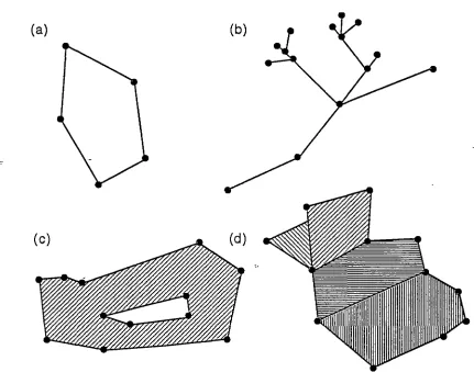
Figure 1.3 - some complex spatial objects for 3-dimensional applications - (a) a ring or I-manifold (b) a complex I-dimensional spatial object (c) a complex
2-dimensional cell (d) a complex 2-2-dimensional spatial object in R3 If the k-cell complex subdivides a k-manifold (a subset of the class of complex spatial objects given above), then intuitively the cells that intersect a 'small'
k-dimensional neighborhood of any j-cell (k-2 ~j ~ k-1) may be ordered 'about' the j-cell. This ordering is consistent because every point of the underlying manifold is guaranteed to have a k-dimensional 'disk' neighbourhood (see the definition of a manifold given above). In practice, the cells that intersect the 'small' k-dimensional neighborhood of the j-cell are the (j+2)-cells and (j+ I)-cells returned by iterative evaluation of the coboundary relation ofj-cell ie. 'the coboundary of the
consists of alternating 0-cells and 1-cells about an abstract cell of dimension -1. Other (well-known) examples include: j
=
0, k=
2 - the circular ordering ofalternating 1-cells and 2-cells about a 0-cell
in
a subdivided 2-manifold;j=
1, k=
2 - since there are no 3-cells in a subdivided 2-manifold the circular ordering degrades to a 'two-sided' ordering consisting of two 2-cells; andj
= 1, k = 3, the circular ordering of alternating 2-cells and 3-cells about a 1-cell in a subdivided 3-manifold. Different directions in these orderings (left, right, clockwise, counter-clockwise etc.) are derived by propagatihg the ordering of the 0-cell boundaries of a 1-cell, to 2-cells and then to 3-2-cells etc.Examples of the 'two-sided' co boundary and the circular orderings formed by 'the co boundary of the coboundary' are shown
in
figures 1.4-1.6. It is particularly interesting to note that for subdivided 3-manifolds (figure 1.5), there is no known ordering of 1-cells, 2-cells and 3-cells in the 3-disk neighborhood of a 0-cell. However there may be more than one circular ordering of 1-cells and 2-cells about such a 0-cell. We refer to such circular orderings as 'subspace' orderings. [image:22.537.101.459.379.695.2](b)
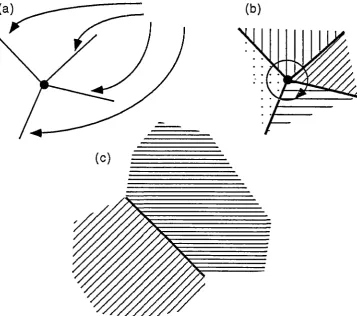
Figure 1.4 - coboundary orderings in a subdivided 2-manifold (a) the coboundary of a 0-cell (b) the circular ordering of 1-cells and 2-cells about the 0-cell and (c)
the coboundary of a 1-cell ie. a 'two-sided' ordering
Coboundary of a 1-cell
l
\
[image:23.540.102.458.168.571.2]~
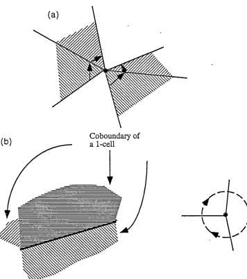
Figure 1.5 - co boundary orderings in a subdivided 3-manifold (a) two subspace circular orderings for a 0-cell (shaded disks when flattened). There is no general ordering of cells, 2-cells and 3-cells about the 0-cell. (b) the coboundary of a 1-cell and an 'end on view' of the circular ordering of 2-1-cells and 3-1-cells about a 1-1-cell.
4, ~-... ~ -~->~-::..~ ...
,.~~.!1'1F'\•~~-(a)
0
Coboundary ofa 0-cell
Figure 1.6 - coboundary orderings in a subdivided 1-manifold (a) the circular ordering of 0-cells and 1-cells about a (-1)-cell (the '(-1)-cell' is not shown for
obvious reasons!) (b) the coboundary of a 0-cell These orderings form a simple and powerful method for traversing all subcomplexes of a cell complex which subdivides- a manifold.
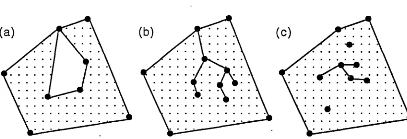
Unfortunately, the spatial objects we described earlier (ie. collections of 'cells') do not necessarily form subdivided manifolds. For example, the tree shown in figure
1.3(b) is not a subdivided 1-manifold and the 2-dimensional spatial object in figure 1.3(c) is not a subdivided 2-manifold. Consequently we cannot make any assertions about the shape of the neighborhoods of all points in the space subdivided by the spatial object and thus, the co boundary orde~ng results cannot be applied to all cells in their cell complexes.
In 2-dimensional GIS applications, the problem is circumvented by 'embedding' the spatial object in a Euclidean 2-manifold which is represented by a special 2-cell of effectively 'infinite extent' known as the 'world' 2-cell. However, if the dimension of the spatial object does not match the Euclidean 2-manifold (eg. in the case of a 1-dimensional spatial object such as a tree) then special cases of the coboundary orderings result. The basis for these special ordering results is the embedding of the spatial object in the Euclidean manifold, guaranteeing that each point has a 2-dimensional disk neighborhood.
We will adopt the same approach in this research: spatial objects will be embedded in a Euclidean 3-manifold (represented by a 'world' 3-cell) in order to obtain the ordering results based on the 3-dimensional 'disk-like' neighborhood. Once again, if the dimension of the spatial object does not match the Euclidean 3-manifold, then special cases of the co boundary orderings result. We shall study the special cases in detail
1.4.2 Relationships between distinct cell complexes
As mentioned above we are also interested in answering questions about spatial relationships between spatial objects. These spatial relationships should be expressed in terms of the cells in the different cell complexes representing the spatial objects (inter cell complex). One solution used in 2-dimensional GIS applications, is to calculate the union of the cell complexes representing the spatial objects. The result is another cell complex, which when embedded in a Euclidean manifold, gives the appropriate ordering results mentioned above (iilcluding any special cases if the spatial objects are not of the same dimension as the Euclidean manifold). If the cell complex results from the union of spatial objects with different dimensions, the cells of this complex differ from those described above in the following ways:
1. The boundary cycles of the cells may no longer be manifolds
2. Cell complexes may be contained within the interior of other cells (ie. besides the 'world' cell).
Cells whose boundary cycles are not simple manifolds will be referred to as singular cells and what we previously referred to as a cell (ie. manifold boundary cycles) is a regular cell. Corbett (1975) & (1979) defined the boundary cycle of a singular cell as the image of a continuous map applied to the boundary cycle of a regular cell which results in the identification of sets of points. This identification is the singularity. Since such a general definition permits a myriad of different
(c)
Figure 1.7 - singular 2-cells (a) 2-cell with a cyclic singular boundary (b) 2-cell With an acyclic singular boundary (c) a 2-cell with interior singularities
The main advantages of using a singular 2-cell complex to represent two or more spatial objects are:
1. The boundary-coboundary relationships between the cells implicitly define the relationships between spatial objects. For example, if a river system (a 1-cell complex) and land tenure boundaries (2-cell complex) are combined within one singular 2-cell complex, then questions such as, whether a river forms the border of, or flows through a property, can be answered by finding at least one 1-cell of the river that has the property as one or both of its co bounding 2-cells, respectively.
2.
A spatial object may itself be multi-dimensional. For example a river
system which contains lakes formed by dams may consist of both areal and linear features.
3.
2-manifolds are 'well-lmown' spaces·in topology. Their properties have been classified and the presence of errors can be detected by checking the ordering of the cell neighbourhood information given above using either the primal or dual constructions. For examples see White (1978) & (1984) and Corbett (1979) and the global concept of planar enforcementFor 3-dimensional applications, the problem of answering questions about spatial relationships between spatial objects will be handled in the same way. That is, a singular 3-cell complex will be formed from the union of the regular cell complexes representing the spatial objects. Each boundary cycle of a singular cell will be defined as a pseudomanifold and can be thought of as the image of a continuous map applied to the manifold boundary of a regular cell. Using an approach similar to that of Corbett (1979), we classify these pseudomanifolds into three primitive
types by applying the theory of Whitney (1944) and identification spaces from topology. The classification reduces the immense range of possibilities to a representative set which provides the basis for the extension of the coboundary ordering results given above, to singular cell complexes.
1.4.3 Representing the Cell Complexes
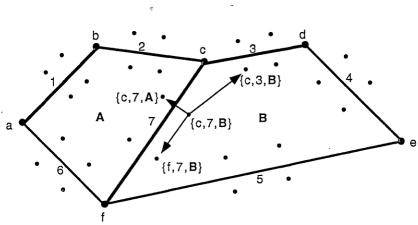
To represent these cell complexes we choose to extend the cell-tuple structure of Brisson t1990). The cell-tuple has the following advantages:
1. Implicit -a cell complex is represented by a set of very simple 'elements'. In this case the 'elements' are tuples of integers representing sets of incident cells. Other topological models which are also implicit (but not to the same extent) include the winged-edge of Baumgart (1974), the face-edge of Hanrahan (1985) and the selective geometric complex of Rossignac and O'Connor (1991).
2. Dimension Independence -The cell-tuple was originally designed to represent subdivisions of n-manifolds. Consequently, the underlying principles are not dependent upon the dimension of the cell complex. Other models such as the winged-edge of Baumgart (1974) or the facet-edge of Dobkin and Laszlo (1987) are dependent upon the dimension of the cell-complex.
3. Coboundary Ordering Information -the cell-tuple structure captures both the boundary-co boundary relations and the ordering information for subdivided manifolds, in a simple graph structure.
1.5 Topological Operators
Operators for traversing and constructing the cell complex are just as important as the description of the representation of spatial objects using a cell complex. We describe these operators as topological operators, because they construct and query the topological relationships between the cells of a cell complex and they are not dependent upon metric concepts.
forming its boundary or its coboundary. It will be shown in chapter 3 and 4 that an extension of the cell-tuple of Brisson (1990) encapsulates these relationships for both regular and singular cell complexes.
The other set of topological operators that we consider are those that allow us to construct the cells and the cell complex. As mentioned earlier in this chapter, a singular cell complex results from the union of one or more regular cell complexes -each of which corresponds to a spatial object Consequently we restrict our attention to the construction of these regular cell complexes (the union process used to form the singular cell complex is a subject for future research). A generic set of
-topological operators for constructing a regular k-cell complex should be able to:
1.
Construct each k-cell (ie. a Euclidean k-manifold with (k-1)-manifoldboundary cycles).
2. Join cells together along subsets of their boundaries in a Euclidean n-manifold
n ;:::
k.The operators described in Corbett (1985) (and by Brisson 1990, but for a more restricted domain) typify this approach and will form the basis of the extensions proposed in this research.
The advantages of this approach are application independence and s4nplicity, since only a small set of operators is required to construct all spatial objects.
A major problem in the construction of spatial objects with such topological - operators is consistency; ie. ensuring that any spatial object falls within the domain
and/or has the required topological properties eg. the correct number of 'holes'. In this research, the problem is compounded by the fact that the domain of spatial objects that we have chosen (see section 1.4) has very few restrictions that could be used for consistency purposes. A 'local' approach to the problem of consistency could be based on ensuring that regular cells are correctly defined and may only be joined along their boundaries in order to form the regular cell complex. Fortunately, we can do better by maintaining consistency across a slightly larger subset of the domain: the subdivided k-manifolds and k-manifolds with boundary (k S: 2). This subset includes regular k-cells, the boundary cycles of regular 3-cells and the boundaries of many 3-dimensional spatial objects. As an example, a set of mine development tunnels with pillars is often represented by a surface which is
topologically equivalent to a subdivided 2-sphere with handles (eg. a torus), where
the number of handles equals the number of pillars. It would be useful to be able to ensure that this surface has the correct number of pillars both before and throughout its construction (not just after).
To achieve consistency across the subdivided manifolds and manifolds with
boundary, we modify the generic cell complex construction operators such that they preserve a very general topological invariant known as the homotopy type (see section 3.2 for a definition). The advantage of this-process is that we can use a very simple space (known as the strong deformation retract) which encapsulates
important topological properties (eg. connectivity) and can be specified as a simple I-dimensional spatial object, prior to the construction of the subdivided manifold or manifold with boundary. The .modified generic construction operators are used to construct the remainder of the subdivided manifold or manifold with boundary from the strong deformation retract whilst preserving its homotopy type, thus maintaining consistency.
The local Euler operators as described in Mantyla (1988) are a special case of this procedure specific to 2-manifolds because they rely on the initial construction of a 2-sphere, and then repeated splitting of 0-cells (ie. adding an edge) and 2-cells (ie. adding a face) within the 2-sphere, to form a subdivided 2-manifold. It will be shown that the local Euler operators actually perform a special restricted form of combinatorial homotopy.
The main disadvantage of the combinatorial homotopy operators is that they only apply to spatial objects in a subset of the domain of the spatial information system. However, a complex spatial object can be constructed using a two stage process. Firstly, the boundary cycles of cells and/or subspaces of the spatial object
from a I-skeleton. In particular, the fundamental group is shown to be essential in extending these algorithms from simple subdivided spheres to subdivided 2-manifolds and 2-2-manifolds with boundary.
1.6 Overview of this Thesis
The three major goals of this research are:
1. To define new cell complexes for representing individual spatial objects and combinations of spatial objects of different dimensions which optimize the representation of their geometric structure and their topological properties but maintain compatibility with the singular and regular cell complexes used in existing spatial information systems.
2. To define a general set of topological operators for consistent construction of a tractable subset of the domain of spatial objects -the subdivided k-manifolds and k-manifolds with boundary (k ~ 2). 3. To extend the simple implicit cell-tuple representation proposed by
Brisson (1990) and the circular ordering results upon which it is based, to the new cell complexes described in this research.
In chapter 2 a simple taxonomy of existing topological models is put forward using the terms introduced in the preceding sections of this chapter. Then the important topological models are individually reviewed.
Chapter 3 presents the mathematical theory underlying this research. After
describing homeomorphism and homotopy, the important topological properties of manifolds and manifolds with boundaries are given.
Chapter 4 reviews the traditional cell complexes used in topology (ie. simplicial, regular CW and normal CW) and then describes the generalized regular cell complex. The generalized regular cell complex is intended to optimize the representation of both the geometric and topological properties of individual uni-dimensional spatial objects, without losing the ability to calculate these properties. The cell-tuple of Brisson (1990) and the underlying circular orderings of
cobounding cells are then extended to generalized regular cells and cell complexes embedded in Euclidean manifolds.
To model spatial objects of different dimensions within the same cell complex, chapter 5 introduces the generalized singular cell complex. The pseudomanifold boundary cycles of these singular cells are classified into three primitive types using identification spaces and the theory of Whitney (1944). The coboundary orderings implied by this classification of pseudomanifolds are then determined and the implicit cell-tuple model is extended to generalized singular cells and cell complexes.
-
-The last section of chapter 5 introduces another cell complex which is based on the normal CW complex described in chapter 4. The cells of this complex are intended to represent the topological structure of the generalized regular and singular cells only. The main advantage is that they achieve a compression of the redundant cell neighborhood information that would normally be held in the generalized regular and singular cell complexes. The cells of this new complex are called '2-arcs' because they are a 2-dimension extension of the 1-arc concept that has been successfully applied in 2-dimensional GIS.
Chapter 6 presents the topological operators for construction of generalized regular and singular cell complexes using the notions of strong deformation retract,
homotopy type, combinatorial homotopy and the generic cell complex construction operators of Corbett (1985) and Brisson (1990). Relationships between the
homotopy type, these operators and various solutions to the automated
reconstruction of a subset of the spaces in the domain (in particular Ganter 1981) are examined.
Chapter 2
Review of Existing
Topolog~cal
Models
2.1 Introduction and Taxonomy of Topological Models
This chapter gives a detailed review of existing topological models using a number of criteria, some of which were briefly mentioned in chapter 1. These criteria give rise to a taxonomy of topological models, but like most taxonomies there are exceptions.
Uni-dimensional Domain vs. Multi-dimensional Domain -In this research, the domain (ie. set of representable spatial objects) of topological models which are able to represent uni-dimensional spatial objects (regular cell complexes) will be referred to as uni-dimensional. The domain of topological models which are able to
represent spatial objects of more than one dimension will be referred to as multi.-dimensional. Multi-dimensional domains must be based on some form of singular cell complex.
Cell Co boundary Orderin !!S -If the domain consists of the subdivided n-manifolds then the coboundary ordering relationships discussed above may be applied to cells of dimension (n-2) or higher. If the domain is larger than the subdivided
n-manifolds then coboundary orderings can only be obtained by 'embedding' the spatial object(s) in a Euclidean manifold of the same of higher dimension. Special cases of the ordering results must be defined.
Implicit vs. Explicit CBrisson 1990) -An implicit model represents the boundary-coboundary neighbourhood relationships of cells in a cell complex using a set of 'elements' eg. winged-edges (Baumgart 1974) or cell-tuples (Brisson 1990). Explicit models usually represent a set of basic 'elements' but also include redundant
'elements', usually to improve retrieval by removing the need to reconstruct certain critical elements (eg. the boundary cycles of polygons and solids). However there are disadvantages to the inclusion of redundant topological elements:
1.
Redundancy complicates the design and increases the storage requirements of the data model (see Milne et al. 1993 for example). Once again the problem is exacerbated in higher-dimensional applications.2. Redundrult spatial objects must be maintained throughout all operations on the model.
3. Redundant spatial objects generally have larger extents than the individual cells they are composed of. Thus they are more likely to be fragmented or cause overlap in the partitions of any spatial access scheme. Fragmentation and overlap in partitioning schemes degrade the retrieval performance that can be gained from any spatial access scheme - see Chapter 8 of Langran (1992) for a review and taxonomy of spatial access schemes.
These disadvantages indicate why very explicit models such as the radial-edge of Weiler (1986) and the tri-cyclic cusp of Gursoz et al. (1991) are not as-attractive for representing 'real-world' or 'geographic' spatial objects as they are for
representing less complicated man-made objects in computer-aided design (Sword 1991).
'
Qill£ -
As was noted in section 1.4, the definition of a 'cell' varies widely from themost restrictive definition in topology, to Euclidean manifolds with boundaries, as we use them in
this research. We will distinguish between the different definitions
used when necessary.2.2 Map Models Used in 2-Dimensional GIS
Overview
Topological models used in 2-dimensional geographic information systems (GIS)
have multi-dimensional domains consisting of 0,1 and 2-dimensional spatial objects embedded in a Euclidean 2-manifold or a space homeomorphic to it, such
as
a mapprojection. The early approaches such as the DIME model of Cooke
&
Maxfield(I967) (see also Corbett I975 & I979) were implicit, storing only the two vertices
bounding and the two coboundary polygons of an edge. Complex spatial objects
were recons_tructed using the circular ordering relationships for a subdivided
2-manifold (see section I.4) and the dual complex (ie. that obtained by substituting
points for polygons, edges for edges and polygons for points). To speed up access
to commonly retrieved spatial objects (eg. boundary cycles of polygons), more
recent models explicitly represent polygon boundary cycles and the cobounding
I-cells of each 0-cell. Examples of such explicit approaches can be found in Chrisman (I975) and in the arc-node model described in Aronoff (I989). A less explicit
approach which is somewhat similar to the winged-edge of Baumgart (I974) is
adopted in the successor to the DIME system, TIGER. In essence, TIGER stores
the same basic boundary-coboundary information
as
the DIME segment except thatinstead of holding the list of boundary I-cells for a polygon as in the arc-node
model, a pointer to the first I-cell in the boundary is stored and each I-cell has _
pointers to the two forward 'wings' forming the next boundary I-cell of the left
polygon and the next boundary I-cell of the right polygon. Polygon boundaries
are
now implicit (as opposed to explicit in the arc-node model) and are reconstructed by'threading' the I-cells together (see Moore I985 and the Arithmicon system of
White I978 for some of the principles behind this approach).
Since all these approaches are variations of the same cells and cell complex we
describe the important underlying principles only using the excellent basis provided
in Corbett (I975) & (I979) and White (I978) ..
Subdivision
The spatial objects are finitized into discrete, piecewise linear n-cells (0 ~
n :::;;
2) each of which (apart from 0-cells) is topologically equivalent to an n-manifold with one or more (n-1)-manifold boundary cycles. When combined in a Euclidean 2-manifold or "world" 2-cell, these spatial objects may intersect. The principleunderlying the cell complex is that no cell intersects another except along their
boundaries. Thus when the cells of spatial objects in the "world" 2-cell intersect, they are subdivided. The effect on 2-cells is that their boundary 1-cycles may also have dangling 1-cell complexes and they may have isolated interior cell complexes (as mentioned in section 1.4).
[image:35.538.80.508.373.636.2]:::~::::)(·::::·::::::
. . .
.
. .
. . . .
. . . .
. . .
....
e • e • • e e • I I I I I I I I I I I I I I
...•...
I I I I I I I I I I I I I I I I I I I I
0
1 I I I I I I I I I I I I I I I I I I I I I I I I I I I I I I I
. . .
. .
. ... .
Figure 2.1 - a singular 2-cell ie. a 2-cell with isolated 1-cells and 0-cells in its interior and a boundary 1-cycle with a dangling tree structure
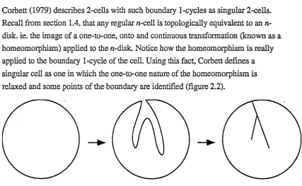
Corbett (1979) describes 2-cells with such boundary 1-cycles as singular 2-cells. Recall from section 1.4, that any regular n-cell is topologically equivalent to an n-disk. ie. the image of a one-to-one, onto and continuous transformation (known as a homeomorphism) applied to the n-disk. Notice how the homeomorphism is really applied to the boundary 1-cycle of the cell. Using this fact, Corbett defines a singular cell as one in which the one-to-one nature of the homeomorphism is relaxed and some points of the boundary are identified (figure 2.2).
Figure 2.2 - formation of a singular cell by defonning its boundary and identifying points (see also White 1984)
Corbett then classifies these singularities into two types: acyclic and cyclic.
such 1-cells may be distinguished (along with any isolated I-cells in the interior of
the 2-cell) by noting that they have the same left and right cobounding 2-cell
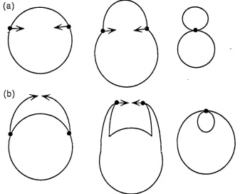
Cyclic singularities may be classified into two types shown in figure 2.3. They are
[image:36.538.112.449.169.441.2]fanned by identifying two points of the boundary 1-cycle.
Figure 2.3 - cyclic singularities generated by identifying points -(a) a 'figure 8' (b) an interior 'hole'
Corbett recognized the importance of the dual complex
as
an alternative method forsolving problems that are more difficult to deal with in the usual (or primal) cell
complex. The dual construction is fanned by 'representing' primal cells by their dual
cells. For example in a subdivided 2-manifold, the primal 2-cells
are
represented bydual 0-cells connected by dual 1-cells (primal 1-cells are self-dual). It is interesting
to note that the two types of singularity classified by Corbett above tum out to be 'duals' of one another in the singular dual cell complex (figure 2.4).
As far as the author knows the full implications of this classification of singular
cells have not been realized or studied in higher dimensions - the principles described in Corbett (1979) and White (1984) fonn the primary basis for the
approach taken to 3-dimensional applications in this research.
\
I
-I\ /
I
I
I
I
\
I /
/~
-
__,
/\ '
... - /-
-\
\
-/
\
//
\
/- -
*~
-\
\
\
[image:37.540.100.419.66.426.2]\
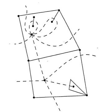
Figure 2.4- a singular cell complex and its dual construction - notice how the two types of singularity defined by Corbett (1979) are 'duals' - see also Guibas and
Stolfi (1985)
Ordering
Corbett (1975) & (1979) and White (1978) were the first to express the
neighbourhood or adjacency information of cells in terms of boundary and
co boundary relationships and specify how the coboundary information may be
ordered. As mentioned above, the DIME structure provides explicit access to the left
and right cobounding polygons of every edge and the boundary vertices or nodes of
the edge and its dual. The DIME structure, like the winged-edge of Baumgart
(1974), is a minimum 'template' of the neighbourhood information. To ease the cost
of processing, other models explicitly store the co bounding edges of a vertex or
node and the boundary edges of polygons.
One of the most important points about the boundary and coboundary operators is
special classes of complex spatial objects for specific applications within the cell complex; eg. route systems for transportation planning and analysis.
2.3 Subdivisions of 2-manifolds
2.3.1 Winged-Edge
Overview
Early topological models for computer-aided design (CAD) systems (also known
as
"boundary" models) were based on that fact that subdivided 2-manifolds 'match' the surfaces of many solid objects. The first 2-manifold topological CAD model
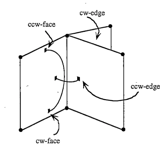
appears to have been devised by Baumgart (1974) and is known as the winged-edge model. The winged-edge is a representation of the 'minimum template' of cells required to capture the boundary-coboundary relationships and coboundary orderings in a subdivided 2-manifold (figure 2.5).
LCCW edge
RCW edge
left
face
right
face
LCW edge
RCCW edge Figure 2.5 - the winged-edge template
For example, to trace the edges of the left face of an edge (a circular ordering), choose either LCW (left-clockwise) or LCCW (left-counter-clockwise) and then move the template to that edge. A well-known disadvantage of the winged-edge representation is that the arbitrary assignment of direction to the edge makes it necessary to test which of LCCW, LCW, RCCW or RCW is the next required edge.
The winged-edge representation is applied to regular 2-cell complexes. However (as we shall see) modifications have been implemented by other authors which permit the winged-edge principle to be applied to singular 2-cell complexes.
Improvements and variations (primarily in space and efficiency) on the winged-edge have been made by various authors (eg. Hanrahan 1985, Weiler 1985, Woo 1985) using modifications of a set of adjacency relationships for subdivided 2-manifolds
devised by Baer et al. (1979). However the underlying principles of the
winged-edge remain the same.
2.3.2 Quad-Edge
Overview
Guibas and Stolfi (1985) introduce an implicit topological model for subdivided
2-manifolds called the quad-edge. However their approach is subtly different to the
usual winged-edge approach of Baumgart (1974). The basic element of their
approach is still the 1-cell, but instead of explicitly representing the left-clockwise
(LCW), left-counter-clockwise (LCCW), right-clockwise (RCW) and
right-counter-clockwise (RCCW) edges (see figure 2.5), they define operators based on
four
possible directed oriented edges that may be associated with any edge in a
subdivided manifold by different orderings of the edge itself and the adjacent
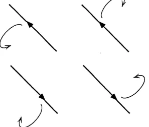
[image:39.540.134.432.353.605.2]2-cell boundaries (figure 2.6).
Figure 2.6 - the four directed oriented edges associated with an edge (from Brisson 1990)
Two operators: One:xt (next edge in either clockwise or counter-clockwise direction as indicated by the orientation of the edge) and Flip (change from a directed
which underlies the claim by Brisson (1990) that the quad-edge is 'more implicit' than the winged-edge.
In addition to the primal cells, Guibas and Stolfi also define and represent the cells of the dual subdivision. An additional, operator Rot (short for rotate ninety degrees) moves between edges in the primal subdivision and edges in the dual subdivision, since edges are self-dual in any subdivision of a 2-manifold.
The term 'quad-edge' arises from the four possible ways of giving orientation to a primal or dual edge and its two cobounding faces.
The cells of the quad-edge may have acyclic singularities as defined by the classification of Corbett (1979) and given in section 2.2. However (as the dual subdivision shown in figure 2.4 shows) there is no r,~ason why the quad-edge could not be extended to singular cells.
Since Brisson (1990) gives both an excellent review and a simple generalization of the quad-edge, it is not necessary to give further details, except to note that Guibas and Stolfi's research forms the foundation of the more recent implicit topological models developed in the field of computational geometry.
2.3.3 Half-Edge
Overview
The half-edge topological model of Mantyla (1988) is a variation of the winged-edge model whi~h represents one or more disjoint subdivided 2-manifolds embedded in a Euclidean 3-manifold. However, the half-edge is a much more explicit model than the winged-edge, since it explicitly represents the boundary cycles of the 1-cells and 2-cells and includes provisions for these 1-cells and 2-cells to be singular. The underlying principles of the model are rigorously based on the fact that any 2-manifold may be represented by a polygon with oriented edges identified in pairs (known as a plane model). The term 'half-edge' originates from the fact that in any subdivided 2-manifold, the two co bounding polygons of an edge represent 'half the neighborhood of an edge.
Subdivision
To represent the vertices, edges and faces in a subdivided 2-manifold, an explicit five-level hierarchical model consisting of the following elements is used.