Collision avoidance as a robust reachability problem under model uncertainty

AAS 16-365

COLLISION AVOIDANCE AS A ROBUST REACHABILITY

PROBLEM UNDER MODEL UNCERTAINTY

Massimiliano Vasile∗_{, Chiara Tardioli}†_{, Annalisa Riccardi}‡ and Hiroshi Yamakawa§

The paper presents an approach to the design of an optimal collision avoidance maneuver under model uncertainty. The dynamical model is assumed to be only partially known and the missing components are modeled with a polynomial ex-pansion whose coefficients are recovered from sparse observations. The resulting optimal control problem is then translated into a robust reachability problem in which a controlled object has to avoid the region of possible collisions, in a given time, with a given target. The paper will present a solution for a circular orbit in the case in which the reachable set is given by the level set of an artificial potential function.

INTRODUCTION

In this work, the problem of avoiding the collision of a controlled object with an uncontrolled target object is translated into a robust reachability problem. The dynamics of the controlled object is assumed to be affected by uncertainty in the dynamic model itself. In orbit determination, a commonly used approach to capture unmodelled accelerations is to introduce so calledempirical accelerationsas additional components to the dynamics. The value of these empirical accelerations can be defined in a number of different ways exploiting the available measurements.

It is customary to use time series expansions in polynomial or trigonometric form whose coeffi-cients need to be found by matching the predication of the model with the observations.1 _Another

approach is to treat empirical accelerations as stochastic processes that can be reconstructed by an approach using a Kalman type of sequential filtering.2

All these techniques generally work satisfactorily and allow one to work with a reduced dynamics without the need for extremely high fidelity models. On the other hand, they do not immediately furnish a functional representation of the missing components. Even using time series expansions, which are valid within the interval in which the measurements are available, to extrapolate the behavior of the dynamical system does not always lead to the desired results. Furthermore, time series do not provide information on the dependency of the empirical accelerations on any of the state variables.

∗

Professor, Department of Mechanical & Aerospace Engineering, University of Strathclyde, 75 Montrose Street, Glasgow, UK.

†

PhD candidate, Department of Mechanical & Aerospace Engineering, University of Strathclyde, 75 Montrose Street, Glasgow, UK.

‡

KE Fellow, Department of Mechanical & Aerospace Engineering, University of Strathclyde, 75 Montrose Street, Glas-gow, UK.

§

For this reason in this paper it is proposed to use polynomial expansions of the state variables instead. The approach proposed in this paper is reminiscent of the approach used in multifidelity modeling to capture model uncertainty via discrepancy functions. As an example in Ng and El-dred,3the discrepancy is modeled with a polynomial chaos expansion under the assumption that the missing component is a stochastic process. Under the same assumption of stochastic unmodelled component, Gaussian mixtures were proposed to capture the distribution of the propagated states.4 In this paper, instead, the missing component in the model is considered to be due to a deterministic process that is only partially observable, or it is observable with some uncertainty.

Once the uncertainty in the dynamic model is quantified, the design of an optimal collision ma-neuver is translated into a robust reachability problem5in which the controlled object has to avoid the region of possible collisions, in a given time, with an uncontrolled target. This problem is translated into a min-max problem and solved with a memetic algorithm.6

As an illustrative example, the paper presents the case of an object moving on a circular low-Earth orbit and subject to a significant unmodelled acceleration component proportional to the square of the velocity.

QUANTIFICATION OF MODEL UNCERTAINTY

Letf :S × P ×[t0 :t0+T] −→Rnandν :S × B ×[t0 :t0+T]−→ Rnbe two vectorial

functions withS ⊆ Rn,B ⊂Rm 0

b andB ⊂ _Rmb_{,n, m}0

b, mb ∈N+. Consider the following initial

value problem

(

˙

s=f(s, b0, t) +ν(s, b, t)

s(t0) =s0 (1)

wheresis the state vector, the mapν(s, b, t) represents some unknown function of the states that is capturing all unmodelled components, b0 ∈ P ⊆ Rm

0

b is a set of uncertain model parameters,

b∈ B ⊆_Rmb _{is some unknown parameter vector of the unmodelled components, andtis the time} coordinate. In this paper, let us restrict ourselves to the case in which the unmodelled components are not a function of time (the case with time dependence is easily obtained from the time inde-pendent formulation). Furthermore, let us consider the special case in which the functionνcan be expressed as

νph(s, b) = 0, νqh(s, b) =Qh =∇phU(s, b) +∇qhU(s, b) (2)

forh= 1, . . . , N, wheres= (p, q)T ∈R2N is the action and moment vector,Q:S × B −→RN,

andU is a continuous and differentiable scalar uncertainty function that can be expanded in the following hierarchical form:

U(s, b)'a(b)0+ 2N X

i

a(b)iξi(si)

+

2N X

i

2N X

j

a(b)ijξij(si, sj) +

2N X

i

2N X

j

2N X

k

a(b)ijkξijk(si, sj, sk) +. . . (3)

witha(b)0, a(b)i, a(b)ij, . . .polynomials in the components ofbonly. If Eq. (1) describes the time

is:

Qh(s, b) = ∂U ∂sh

'

2N X

i

a(b)i+

2N X

i ζi(si)

+

2N X

i

2N X

j

ζij(si, sj) +

2N X

i

2N X

j

2N X

k

ζijk(si, sj, sk) +. . . (4)

with ζi = a(b)ih∂ξih/∂sh +a(b)hi∂ξhi/∂sh, fori = 1, . . . ,2N, and so on. Ifξ are monomial

bases, then the generalised force reads:

Qh(s, b)'c0+ 2N X

i

c(b)i∆si

+

2N X

i

2N X

j

c(b)ij∆si∆sj+

2N X

i

2N X

j

2N X

k

c(b)ijk∆si∆sj∆sk+. . . (5)

with c0 = P2iNa(b)i and c(b)i, c(b)ij, . . . polynomials in b. Let us indicate with l ∈ N+ the

dimension of the vectorc= (c0, c(b)1, . . . , c(b)2N, c(b)11, . . .)T.

Problem Statement

GivenQand a set of observations, one can obtain an approximated representation of the unmod-elled components by finding the value ofcthat best fits the measurements. Then, the value of the coefficients of expansion (4) can be obtained as the solution of an optimisation problem. The na-ture of the optimisation problem slightly differs depending on the integration scheme used to solve Eq. (1). If No exact and distinct measurements are available then one needs to solve the set of

constraints

s(ti, c)−so(ti) = 0, i= 1, . . . , No, (6)

wheres(ti, c) is the propagated state at timeti andso(ti) is the observed state at timeti. If the number of observationsNois equal tol, the number of coefficients in expansion (4), one could argue

that the solution of problem (6) provides the exact values of all the components of c. Constraint equations (6) can be solved in a least square sense by solving:

min

c [s(t, c)−so(t)]

T_{[s(t, c)−s}

o(t)] (7)

Alternatively, if No < l, a suitable smoothing function can be introduced and the following problem needs to be solved:

min

c J(s, c)

s.t. s(ti, c)−so(ti) = 0, i= 1, . . . , No, (8)

whereJ :S × C −→_Ris a real function of statess∈S⊂_Rn_{and coefficientsc∈C ⊂}

Rl. Note

Treatment of Stochastic Observations

The interest in this paper is to reconstruct the missing components from a small set of sparse observations over possibly long arcs. In the case of observations affected by an error, one cannot obtain a prediction of the exact value of the parametersc. In this case, it is reasonable to assume that the initial conditions are also uncertain as they come from previous observations. If the expected values of the state vector, coming from observations, are enforced as hard constraints the result might not capture the actual missing components as the trajectory is forced to satisfy constraints that do not come from the natural dynamics but are dependent on the errors in the observations. One option is to consider the most probable value for each observation and a cost function that maximises the likelihood of correct identification. The other option is to quantify the uncertainty in the observations and initial conditions as confidence intervals on the observed states. More formally, consider the uncertainty space(Γ,L,M), withΓa non empty set, La σ-algebra overΓ, andM an uncertainty measure. Then the observed state is an uncertainty variableso : (Γ,L,M)−→ Rn.

If the distribution ofso is available, one can drawNp samples and solve problem (8)Np times to

derive a distribution of the coefficientsc. Alternatively, if no distribution is available forso, butΣis

the collection of all the confidence intervals for all the observations, including the initial conditions, such that

P r(so ∈Σ)> ε , (9)

withε >0, then one can formulate the following optimisation problem:

min

c∈C J(s, c)

s.t. s(ti)∈Σ, i= 0, . . . , No.

(10)

The main advantage of this formulation is that no statistical moments are required, and no exact distribution needs to be known a priori. Note that the initial conditions s(t0) are treated as an

observed state.

The objective function in Eq. (10) can be interpreted as a distance in the metric vector spaceCof the parametersc. In this space, the origin represents the solution with no model uncertainty and any point at distance√cT_{cfrom the origin has uncertainty vectorQanduncertainty distance:}

du = Z

QTQ dt . (11)

MODEL UNCERTAINTY IN ORBITAL DYNAMICS

As an example, we take the case of a spacecraft in low-Earth orbit. The gravity component of the model is fully known, but the observations show an additional component that is not modeled. The real dynamics is governed by the following system of differential equations written in Hill’s variables:7

˙

r=vr

˙

u=G/r2−rcosIsinuFn/(GsinI)

˙

h=rsinuFn/(GsinI) (12)

˙

vr=G2/r3−µ/r2+Fr

˙

G=rFu

˙

whereFr, Fu, Fn are the component of the non-gravitational forces in the radial, transversal, and out-of-plane reference frame.

The Hill variables{r, u, h, vr, G, H}are canonical variables introduced into satellite orbit theory by Izsak7in 1963. They represent, respectively, the radial distance, the argument of pericentre, the longitude of the ascending node, the radial velocity, the absolute value of the angular momentum, and thez-component of the angular momentum. The elements are illustrate in Figure 1.

N  

X  

Y   O  

Z  

e_r   e_n   eu  

r  

u   Ω  

I

Figure 1: Reference frame(er, eu, en)

The governing equations (12) can be re-written in the following form that explicitly introduces the transversal velocityvu, withvu=G/r:

˙

r=vr

˙

u=vu/r−rcosIsinuFn/(rvusinI)

˙

h=rsinuFn/(rvusinI) (13)

˙

vr=v2u/r−µ/r2+Fr

˙

vu=Fu−vrvu/r

˙

H=rcosIFu−rsinIcosuFn

In our example, the non-gravitational force isF =−Cd|v|v, with|v|2 =vr2+vu2, andvn= 0. We

assume a constant value forCd = 0.5·10−6 km−1 so that an appreciable variation of the orbit is

obtained already after one orbit. Furthermore, we assume that the measured variation is with respect to a nominal circular orbit withvr(t = 0) = vr0 = 0andvu(t = 0) = vt0. The orbital period,

without unmodelled force, is T = 2πpr3_{/µ. Substituting the expression ofF in Eqs. (13), the}

vectorial field becomes

˙

r=vr

˙

u=vu/r

˙

h= 0 (14)

˙

vr=v2_u/r−µ/r2−Cd|v|vr

˙

vu=−Cd|v|vu−vrvu/r

˙

In order to capture the unmodelled dynamics, we consider an expansion ofQof the following form

Qr=c1+c3r+c5r2+c7ru+c9vr+c11v2r+c13vrvu

Qu=c2+c4u+c6u2+c8ru+c10vu+c12vu2+c14vrvu (15)

Qn= 0

where Qn is zero because it is assumed that the unmodelled component acts only in-plane, and ci ∈ R, i = 1, . . . ,14. Equation (15) is an incomplete expansion of (5) when the generalised

potentialU in (3) is truncated at the third order. The vectorial field (14) is then expanded as

˙

r =vr

˙

u=vu/r

˙

h= 0 (16)

˙

vr =v2u/r−µ/r2+c1+c3r+c5r2+c7ru+c9vr+c11vr2+c13vrvu

˙

vu =c2+c4u+c6u2+c8ru+c10vu+c12v2u+c14vrvu−vrvu/r

˙

H =rcosI(c2+c4u+c6u2+c8ru+c10vu+c12v2u+c14vrvu)

If the linear effects in Eq. (14) are dominant over a given time span∆t, and there is no out-of-plane component, then the prediction given by Eq. (16) should be of the form:

˙

r=vr

˙

u=vu/r

˙

h= 0 (17)

˙

vr=v2_u/r−µ/r2+c13vrvu

˙

vu=−vuvr/r+c12v2u

˙

H=rcosI c12v2u

We can now introduce observations at time t = T and t = T /2, for a total of 8 constraint equations and 14 parameters. If measurements are affected by an error, problem (10) needs to be solved under some assumptions on the initial conditions. The assumption in this paper is that the initial conditions are taken over a given interval. The size of the confidence on each state variable for the initial conditions and for each observation isr ∈ [¯r −0.01,r¯+ 0.01] km, u ∈

[¯u−10−5,u¯ + 10−5]rad, h ∈ [¯h−10−5,¯h+ 10−5] rad, vr ∈ [¯vr −10−5,¯vr+ 10−5]km/s,

vu ∈[¯vu−10−5,vu¯ + 10−5]km/s,H ∈[ ¯H−10−5,H¯ + 10−5]km2/s, which is consistent with a good orbit determination process, wherer,¯ u,¯ ¯h,¯vr,¯vu,H¯ are the exact values.

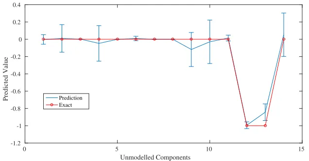
The estimatedcparameters are represented in Figure 2 together with their associated confidence intervals. As one can see, the expected value is close to the expected true solution. One thing that has to be taken into consideration is that the dynamics that are simulated and measured are the true dynamics, not the approximated equations (14). Therefore, some components that are not in the approximated model (14) might be different from zero.

0 5 10 15 Unmodelled Components

-1.2 -1 -0.8 -0.6 -0.4 -0.2 0 0.2 0.4

Predicted Value Prediction Exact

Figure 2: Example of reconstructed gravity-drag dynamics with confidence intervals

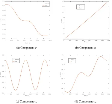
predict the future evolution of the orbit over another period. The resulting trajectory over two orbits is shown in Figures 3.

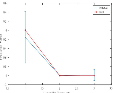
The match between the predicted and the true trajectory is very good although a 2 km error in radius accumulated by the end of the second orbit. Once a first estimation of the coefficient is available, one can iterate the process progressively removing the coefficients that fall below a given threshold. Given the result in Figure 2, one can take all the coefficients with an absolute mean value higher than 0.1 and solve problem (10) once again. From Figure 2 coefficientsc9, c12andc13can

be retained, and Eqs. (16) becomes:

˙

r=vr

˙

u=vu/r

˙

h= 0 (18)

˙

vr=v_u2/r−µ/r2+c9vr+c13vrvu

˙

vu =c12v2u−vrvu/r

˙

H=rcosI c12vu2

After solving problem (10) only with three coefficients, the result is represented in Figure 4. Even in this case after predicting the dynamics over one orbit, one can study the evolution over a second orbit. The absolute error between predicted and true trajectory can be seen in Figure 5.

A REACHABILITY PROBLEM

Once the reachable sets of the controlled and uncontrolled objects are available, a collision avoid-ance maneuver is calculated solving the following min-max optimal control problem:

min

w∈Amaxc∈Ξ ψ(s(tf), w, c, tf)

s.t s˙=f(s, p) +ν(s, b) +g(s, w)

s(t0)∈Σ0

(19)

whereψis a real function,Σ0is the set of possible initial conditions,Ξis the set in which the

0 2000 4000 6000 8000 10000 12000 14000

Time [s] 6900

7000 7100 7200 7300 7400 7500 7600 7700

r [km]

Prediction Exact

(a) Componentr

0 2000 4000 6000 8000 10000 12000 14000 Time [s]

0 2 4 6 8 10 12 14

u [rad]

Prediction

Exact

(b) Componentu

0 2000 4000 6000 8000 10000 12000 14000

Time [s]

-0.12 -0.1 -0.08 -0.06 -0.04 -0.02 0 0.02

vr

[km/s]

Prediction

Exact

(c) Componentvr

0 2000 4000 6000 8000 10000 12000 14000

Time [s]

7.2 7.25 7.3 7.35 7.4 7.45 7.5 7.55 7.6

vu

[km/s]

Prediction Exact

(d) Componentvu

Figure 3: Comparison between the true and predicted estimates.

in the dynamics given by Eqs. (2)–(3),g is the control function, andAis the space of admissible controls. The functionψ(s(tf), w, c, tf)defines whether the terminal state is admissible or not. In other words the reachable set is defined by a level set ofψ.

Artificial potential

Since the interest is to avoid a collision the desired reachable set is the space outside the uncon-trolled target. Thus the functionψ has to be negative or null when a collision occurs and strictly positive otherwise. We started from a tessellation of the region describing the object. A tessellation is a tiling of the space using one or more geometrical shapes, called tiles, with no overlaps and no gaps. An example is a tiling with cubes. LetU be the region to cover andD1, . . . , Dmthe polyhedra

used as tiles. Letnbe the dimension of the space andq > n+ 1 be the number of facets of the polyhedron. We are assuming that the polyhedra in the tessellation are of the same type, however, our dissertation can be extended to the case of a tessellation with different polyhedra.

Each facet can be represented by an hyperplane of equationA(_kj)·(x−xj) = b(_kj), withA(_kj) ∈

0.5 1 1.5 2 2.5 3 3.5 Unmodelled Components

-1.2 -1 -0.8 -0.6 -0.4 -0.2 0 0.2 0.4 0.6

Predicted Value

Prediction Exact

Figure 4: Prediction of the coefficients for the reduced model

the semi-planeA(_kj)·(x−xj)≤b(_kj)contains the centerxjfor eachk, j. Indicating withKjthe set

{k : A(_kj)·(x−xj)−b(_kj) >0}, the function

φj(x) =    

  

− 1

1 +||x−xj||3

, ifK_j =∅,

X

k∈Kj

(A(_kj)(x−xj)−b(kj)), otherwise,

(20)

is such thatφj(x)>0ifxis outside every semi-plane, that is outsideDj, and it isφj(x) ≤0ifx

is inside or on the border ofDj. We note that function (20) is discontinuous on the border ofDj,

however, continuity is not a requirement for our study. We callφj artificial potential of Dj. An

example is shown in Figure 6.

Using the tessellation, the setUis approximated with the union of disjoint setsDj, j = 1, . . . , m, and the artificial potential on this set is defined as

Φ(x) =

      

     

−

m X

j=1

1 1 +||x−xj||3

, ifKj =∅for somej

m X

j=1

X

k∈Kj

(A(_kj)(x−xj)−b(kj)), otherwise

(21)

and satisfies the requirement:

Φ(x) =

≤0, ifx∈D1∪. . .∪Dm,

>0, otherwise. (22)

Superquadratic functions can be used as an alternative to the use of hyperplanes:

ϕj : x₁−x

(j) 1

r1

+. . .+x_n−x(_nj)

rn₋

1, (23)

where xj = (x(₁j), . . . , xn(j)) is the center of Dj, and r1, . . . , rn are positive real numbers. For

0 2000 4000 6000 8000 10000 12000 14000

Time [s]

-0.02 -0.015 -0.01 -0.005 0 0.005

0.01 0.015

∆

r [km]

(a) Componentr

0 2000 4000 6000 8000 10000 12000 14000

Time [s]

-4 -2 0 2 4 6 8

∆

u [rad]

×10-6

(b) Componentu

0 2000 4000 6000 8000 10000 12000 14000

Time [s] -2.5

-2 -1.5 -1 -0.5 0 0.5 1 1.5 2

∆

vr

[km/s]

×10-5

(c) Componentvr

0 2000 4000 6000 8000 10000 12000 14000

Time [s]

-2 -1.5 -1 -0.5 0 0.5 1 1.5

∆

vu

[km/s]

×10-5

(d) Componentvu

Figure 5: Difference between the true and predicted estimates.

one could use the superellipsoid

ϕ0_j :

x1−x(₁j)

r

+x2−x(₂j)

rt/r

+x3−x(₃j)

t

−1, (24)

withr, treal numbers that depends onxj. Then, we set

Φ(x) =

    

   

− X

j=1,...,m

1 1 +||x−xj||3

, ifϕj◦τj(x)≤0for somej

X

j=1,...,m

ϕj(x), otherwise,

(25)

-9-8-7 -6 -5 -4

-3

-3

-2 -2

-1 -1

0

0

0

1

1

1

1

1

2

2

2

2

2 2

2

3 3

3 3

x

-3 -2 -1 0 1 2 3

y

-3 -2 -1 0 1 2 3

Φ(x,y)

(a)

x

-4 -3 -2 -1 0 1 2 3 4

y

-10 -8 -6 -4 -2 0 2 4 5

Φ(x,0)

(b)

Figure 6: Level curves of the pesudo potential on the cube[−1,1]2(a) and the corresponding values

along thex-axis

Solution Approach

The algorithm proposed in this paper to solve min-max problem (19) is a combination of the one proposed in Vasile6_{and Marzat et al.}8_{In Marzat,}8_{the generic unconstrained min-max problem:}

min

d∈Dmaxξ∈U f(d, ξ)

is computed by solving iteratively the following two problems, one after the other:

ξa= argmaxξ∈Uf(dmin, ξ) (26)

dmin = argmind∈D

max

ξa∈Aξ

f(d, ξa) (27)

where the archiveAξis a collection of all theξagenerated by the solution of problem (26) for each newdmin generated by the solution of problem (27). Problem (26) can be seen as a restoration of

the maximum condition on U, therefore the whole process can be considered as a minimisation-restorationloop.

It is important, at this point, to observe that, if a population-based method is used to solve prob-lem (27), subprobprob-lemmaxξa∈Aξf(d, ξa)can be interpreted as a cross-check of theξ associated to a populationP ofdvalues as in Vasile.6 For eachd, in fact, problem (27) requires selecting the

ξa,max that maximizesf among all theξafound thus far. This principle is equivalent to the Nash

The whole process, therefore, might iterate for a long time between minimization and restoration without converging. This is what can be calledred queen effect.

Here, it is proposed to solve both problems (26) and (27) with Inflationary Differential Evo-lution Algorithm (IDEA)10 and to allow the algorithm to compute for each da local maximum

ξ_a,max∗ starting from each element inAξ. The valuedminwith associated local maximumξ∗a,max=

argmax_ξ∗

a∈Uf(dmin, ξ

∗

a), are then saved in the archiveAdand the elements in the archiveAdare

cross-checked to maximise the change to identify the global maximum inU. The overall strategy is presented in Algorithms 1, 2, and 3.

Algorithm 1IDEAminmax

Initialized¯at random and runξa= argmaxξ∈Uf( ¯d, ξ) Aξ=AξS

{ξa}

whilenf eval< nf eval,maxdo

Rundmin= argmind∈D{maxξ∗

a∈A∗ξf(d, ξ

∗ a)}

Runξa= argmaxξ∈Uf(dmin, ξ) iff(dmin, ξa,max∗ )< f(dmin, ξa)then

Aξ=AξS{ξa},Ad=AdS{dmin, ξa} else

Aξ=AξS{ξa,max∗ },Ad=AdS{dmin, ξa,max∗ } end if

end while

Run Cross Check Algorithm 3 over the archiveAd

Algorithm 2maxξ∗

a∈A∗ξf(d, ξ

∗ a)

forall the elements inAξdo

Run local search fromξa∈Aξand computeξ_a∗ = argmaxξ∈Uf(dmin, ξ)

Add local maximum to the set of local maximaA∗_ξ =A∗_ξS_{ ξ_a∗}

end for

ξ∗_a,max= argmax_ξ∗

a∈A∗ξf(dmin, ξ

∗ a)

Algorithm 3Cross Check Initialize∆,ε >0

while∆> εdo

forall the elements inAddo

Compute local maximumf(di, ξj∗)fromξj ∈Ad

∆ =f(di, ξj∗)−f(di, ξi) if∆> εthen

Numerical Examples

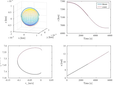
For the sake of illustrating the approach proposed in the previous sections, we consider the case in which after the identification of the missing component, a manoeuvre is required to avoid the col-lision with a known, though uncontrolled object. We say that a colcol-lision occurs when the artificial potential in Eq. (21) is non-positive. For this exercise we consider the position of the two objects projected onto the b-plane at the expected time of impact. The impact occurs almost one orbit af-ter the last measurement is acquired. A low-thrust manoeuvre is then applied to avoid the collision. Since a negative artificial potential corresponds to a collision and a positive artificial potential corre-sponds to no collision, the problem translates into finding the optimal control profile that maximises the artificial potential (21). At the same time, given the uncertainty on the coefficientsc, an optimal and robust control policy has to account for the worst-case value ofc.

The reachability problem then reads:

min

w∈Wmaxc∈Ξ ψ(r, u, h, vr, vu, H, w, c, ti, tf)

s.t. r˙=vr

˙

u=vt/r−cosIsinu wn/(vusinI) ˙

h= sinuwn/(vusinI) ˙

vr =vu2/r−µ/r2+c1vr+c3vrvu+wr

˙

vu =c2vu2−vrvu/r+wu

˙

H =rcosI(c2vu2+wu)−rsinIcosuwn s(t0)∈Σ0

(28)

where (r, u, h, vr, vu, H)T are the Hill variables, w = (wr, wu, wn) is the control acceleration,

c= (c1, c2, c3)are the unknown coefficients in the dynamics, andti, tf are a generic instant of time

and the final time, respectively. The control acceleration is the decision vectorwdescribed in the previous section, and thec is the uncertain vectorξ. Each component of the control acceleration is modeled as a fourth order polynomial, collocated at five points in time along the trajectory. The differential equations in (28) are integrated forward in time with a Runge-Kutta 4/5 order scheme with variable step size.

Figure 7 shows the uncertainty region of the controlled object due to the uncertainty on the co-efficientsc1, c2, c3and initial conditions. Before the manoeuvre, the projection of the uncontrolled

object on the target plane is in the origin of axis, and the level curves of the artificial potential are shown in Figure 8. We considered two cases, one in which the admissible control spaceW is a box with edge[−10−5,10−5]m/s2, the other in which the edge is[−4×10−6,4×10−6]m/s2. The propagation of the position is given in Figure 9, where we also observe that the low-trust (thick solid line) is on for half period, and it has the effect to lower the radial distance.

FINAL REMARKS

-1010191816151413121120-1-2-7-917-6-4-3-8-51209876435

-30 -20 -10 0 10 20 30

ξ [m] -400

-300 -200 -100 0 100 200 300 400

ζ

[m]

-10 -5 0 5 10 15 20

(a)

-9-8 -7-6-5-4 -3 -2 -10123456789 10 11 12 13 14 15 16 17 18 19 20

0 20 40 60 80

ξ [m]

-600 -500 -400 -300 -200 -100 0

ζ

[m]

-10 -5 0 5 10 15 20

Target

(b)

0 10 20 30 40 50

ξ [m] -400

-300 -200 -100 0 100

ζ

[m]

-100 10 2020

-10 -5 0 5 10 15 20 25 30

Target

(c)

Figure 7: Uncertainty region on the b-plane: (a) no manoeuvre (b) post-manoeuvre with maximum

acceleration along each component of10−5 m/s2 (c) post-manoeuvre with maximum acceleration along each component of4×10−6 _m/s2

The use of polynomial expansions is reminiscent of the use of polynomial chaos expansions in multifidelity modeling to represent discrepancies in the model. This form of polynomial representa-tion was demonstrated to well capture the missing part of the dynamics in the case of a circular orbit and a force component proportional to the square of the orbital velocity. Note that exact distribution needs to be known a priori on boundary conditions and observed states.

Besides, once the predicted dynamics is available, the reachable set of an uncontrolled object at different timest∈[to, tf]can be approximated with one of the techniques proposed in Ricciardi et

al.,11starting from the level set of an artificial potential. Likewise, the reachable set of a controlled object can be computed for the same time interval to assess the probability of a collision. In this way, the computation time is drastically reduced, especially in the optimisation part.

ACKNOWLEDGMENT

-10 -10 -10 -10 -10 -10 -10 -9 -9 -9 -9 -9 -9 -9 -8 -8 -8 -8 -8 -8 -8 -7 -7 -7 -7 -7 -7 -7 -6 -6 -6 -6 -6 -6 -6 -5 -5 -5 -5 -5 -5 -5 -4 -4 -4 -4 -4 -4 -4 -4 -3 -3 -3 -3 -3 -3 -3 -3 -2 -2 -2 -2 -2 -2 -2 -2 -1 -1 -1 -1 -1 -1 -1 -1 0 0 0 0 0 0 0 0 1 1 1 1 1 1 1 1 2 2 2 2 2 2 2 2 3 3 3 3 3 3 3 3 4 4 4 4 4 4 4 4 5 5 5 5 5 5 5 5 6 6 6 6 6 6 6 6 7 7 7 7 7 7 7 8 8 8 8 8 8 8 9 9 9 9 9 9 9 10 10 10 10 10 10 10 10 11 11 11 11 11 11 11 11 12 12 12 12 12 12 12 12 12 13 13 13 13 13 13 13 13 13 13 14 14 14 14 14 14 14 14 14 14 15 15 15 15 15 15 15 15 15 15 16 16 16 16 16 16 16 16 16 16 17 17 17 17 17 17 17 17 17 17 18 18 18 18 18 18 18 18 18 18 19 19 19 19 19 19 19 19 19 19 20 20 20 20 20 20 20 20 20 20

-2 0 2

ξ [m] -3 -2 -1 0 1 2 3 4 ζ [m] -10 -5 0 5 10 15 20 (a) -10 -10 -10 -10 -10 -10 -10 -9 -9 -9 -9 -9 -9 -9 -8 -8 -8 -8 -8 -8 -8 -7 -7 -7 -7 -7 -7 -7 -7 -6 -6 -6 -6 -6 -6 -6 -6 -5 -5 -5 -5 -5 -5 -5 -5 -5 -4 -4 -4 -4 -4 -4 -4 -4 -4 -3 -3 -3 -3 -3 -3 -3 -3 -3 -2 -2 -2 -2 -2 -2 -2 -2 -2 -1 -1 -1 -1 -1 -1 -1 -1 -1 0 0 0 0 0 0 0 0 0 1 1 1 1 1 1 1 1 1 2 2 2 2 2 2 2 2 2 3 3 3 3 3 3 3 3 3 4 4 4 4 4 4 4 4 4 5 5 5 5 5 5 5 5 5 6 6 6 6 6 6 6 6 6 7 7 7 7 7 7 7 7 7 8 8 8 8 8 8 8 8 8 9 9 9 9 9 9 9 9 10 10 10 10 10 10 10 10 11 11 11 11 11 11 11 12 12 12 12 12 12 12 13 13 13 13 13 13 13 14 14 14 14 14 14 14 15 15 15 15 15 15 15 15 16 16 16 16 16 16 16 16 17 17 17 17 17 17 17 17 18 18 18 18 18 18 18 18 18 19 19 19 19 19 19 19 19 19 20 20 20 20 20 20 20 20 20

-2 0 2

ξ [m]

-3 -2 -1 0 1 2 3 4 ζ [m] -10 -5 0 5 10 15 20 (b)

Figure 8: Level curves of the pesudo potential for: (a) a cross built with cubes projected on the

b-plane (b) a cross built with super-ellipses projected on the b-plane

number L15548.

REFERENCES

[1] E. M. Alessi, S. Cicalo, and A. Milani, “Accelerometer Data Handling for the BepiColombo Orbit Determination,”Advances in the Astronautical Sciences, Vol. 145, 2012, pp. 121–129.

[2] O. Montenbruck, T. Helleputte, R. Kroes, and E. Gill, “Reduced dynamic orbit determination using GPS code and carrier measurements,”Aerospace Science and Technology, Vol. 9, 2005, pp. 261–271. [3] L. W. T. Ng and M. S. Eldred, “Multifidelity Uncertainty Quantification Using Non-Intrusive

Polyno-mial Chaos and Stochastic Collocation,”Proceedings of the 53rd AIAA/ASME/ASCE/AHS/ASC

Struc-tures, Structural Dynamics and Materials Conference, Honolulu, Hawaii, 23-26 April 2012. AIAA

2012-1852.

[4] D. Giza, P. Singla, and M. Jah, “An Approach for Nonlinear Uncertainty Propagation: Application to Orbital Mechanics,”AIAA Guidance, Navigation, and Control Conference, Chicago, Illinois, USA, 10-13 August 2009 2009.

[5] I. Hwang, D. Stipanovic, and C. Tomlin, “Polytopic Approximations of Reachable Sets Applied to Linear Dynamic Games and a Class of Nonlinear Systems,”Advances in Control, Communication

Net-works, and Transportation Systems, 2005, pp. 3–19.

[6] M. Vasile, “On the solution of min-max problems in robust optimization,”The EVOLVE 2014

Interna-tional Conference, A Bridge between Probability, Set Oriented Numerics, and Evolutionary Computing,

Beijing, July 2014.

[7] I. G. Izsak, “A Note on Perturbation Theory,” Astron. J., Vol. 68, Oct. 1963, pp. 559–561, 10.1086/109180.

[8] J. Marzat, E. Walter, and H. Piet-Lahanier, “A new strategy for worst-case design from costly numerical simulations,”American Control Conference (ACC), 2013, June 2013, pp. 3991–3996.

[9] D. D. Dumitrescu, R. I. Lung, and T. D. Mihoc, “Meta-Rationality in Normal Form Games,”

Interna-tional Journal of Computers Communications & Control, Vol. 5, No. 5, 2010.

[10] M. Vasile, E. Minisci, and M. Locatelli, “An inflationary differential evolution algorithm for space trajectory optimization,”IEEE Transactions on Evolutionary Computation, 2011.

[11] A. Riccardi, C. Tardioli, and M. Vasile, “An intrusive approach to uncertainty propagation in orbital mechanics based on Tchebycheff polynomial algebra,”AAS Astrodynamics Specialists Conference, Vail,

1

y [km]×10

4 0

-1 -0.5 0

×104

z [km]

0.5

-1

×104 x [km]

1

0 ₁ -1 _{0 2000 4000 6000}

Time [s] 6900

7000 7100 7200 7300

r [km]

thrust coast

-0.15 -0.1 -0.05 0 0.05

v

r [m/s]

7.35 7.4 7.45 7.5 7.55 7.6

v u

[km/s]

0 2000 4000 6000

Time [s] 6

8 10 12 14

u [rad]